An Analysis Procedure for Advanced Propulsor Design
by
Dirk Hampton Renick
Submitted to the Departments of Ocean Engineering and Mechanical Engineering in partial fulfillment of the requirements for the degrees of
Naval Engineers Degree
and
Master of Science in Mechanical Engineering
at the
MASSACHUSETTS INSTITUTE OF TECHNOLOGY
egho
arby prtio M
f
permisbn~
axo
andto
May 1999
@Dirk Hamptn'Renick, 1999. All rights reserved.
Il
PDA
Author ...
...
Departments of Ocean Engineering and Mechanical Engineering
May 18, 1999
Certified by .... ... ... ...
Justin E. Kerwin Professor of Naval Architecture Thesis Supervisor
Accepted by ...
Read by...
a/
..
...
Art Baggeroer
Chairman, Department Committee on Graduate Students
...
Douglas P. Hart
Associate Professor of Mechanical Engineering
Theis Reader
A ccepted by ... ... . . . ...
Ain A. Sonin
Professor Chairman, D epartmental Committee on Graduate Studies
MASSACHUSETTS INSTITUTE OF TECHNOLOGY
-9
C'!"'
" I
An Analysis Procedure for Advanced Propulsor Design
by
Dirk Hampton Renick
Submitted to the Departments of Ocean Engineering and Mechanical Engineering on May 18, 1999, in partial fulfillment of the
requirements for the degrees of Naval Engineers Degree
and
Master of Science in Mechanical Engineering
Abstract
A propeller which operates in the shear flow found near the aft end of marine vehicles experiences an intimate coupling between the propeller's induced velocity field and the rotational inflow. The presence of the propeller's induced velocity field causes the inflow to accelerate, which redistributes the vorticity present in the inflow. This redistribution causes a change in the nominal propeller inflow. Because the propeller now experiences a different inflow, the propeller induced velocity field is altered. Thus, there is an intimate coupling between the vorticity present in the fluid inflow and the propeller-generated induced velocity field.
Lifting surface propeller blade design codes are incapable of analytically representing the vortical interaction between the induced velocity field and the rotational inflow. An additional difficulty is encountered as downstream blade elements, which would be present in a multi-component propulsor, pass through the singularity wake sheets shed by upstream components. For these reasons, the propeller blade design code should be coupled with an external flow solver which is capable of transporting vorticity.
Previous researchers have coupled propeller blade design codes with Reynolds Averaged Navier Stokes (RANS) flow solvers. This powerful method made possible multi-element propulsor design in the presence of rotational inflow. Unfortunately, the use of a RANS code is costly in terms of time and computational resources.
This thesis focuses on coupling a propeller blade design code with an axisymmetric, multi-element through-flow code, developed by Drela. The throughflow code uses an integral boundary layer method to solve for the boundary layer flow, and a streamline curvature formulation to solve for the inviscid, outer flow. The main advantage of the present method over previous methods is an order of magnitude reduction in computation time. Validation cases were performed to validate the various components of the coupling procedure, as well as the coupling methodology as a whole. A design case is presented which shows the use of this methodology in design.
Thesis Supervisor: Justin E. Kerwin Title: Professor of Naval Architecture
Acknowledgments
This thesis and the underlying research would not have been possible without the unwavering, solid
support of my wife Naoko, who worried with me every step of the way, offered encouragement when
needed, and lay my head gently to rest every night for these three years. My parents gave me the
tools and the background to succeed. My friends always showed that there was a way other than
my own. My mentors showed me the broader paths. My past teachers taught me to think.
Professor Justin Kerwin, Dr. Todd Taylor, Rich Kimball and Gerard McHugh provided invaluable
insight and guidance into the sometimes black art of propeller blade design and the nuances of
coupling a propeller blade design code with a throughflow solver. Their insightful answers to my
steady barrage of questions led to the successful completion of this thesis.
Contents
1 This Thesis in the Propeller Design Process 12
1.1 Fluid Velocity Terminology . . . . 12
1.2 Effective Inflow . . . . 13
1.3 The Coupled Hull Flow Resistance Problem . . . . 14
1.4 Modern Design Techniques . . . . 14
1.5 Lifting-Surface Propeller Blade Design and Analysis . . . . 16
1.6 Coupling with a Viscous Throughflow Solver . . . . 17
2 Flow Theory 19 2.1 Computational Solution to Fluid Flow Problems . . . . 19
2.1.1 The Boundary Layer Equations . . . . 19
2.2 Streamline Curvature Method . . . . 21
2.2.1 The Original Streamline Curvature Method . . . . 21
2.2.2 Finite Volume Formulation . . . . 22
2.2.3 Drela's Throughflow Formulation . . . . 23
2.3 IBLT Boundary Layer Representation . . . . 24
2.3.1
IBLT Diffculties . . . .
24
3 Coupling PBD and MTFLOW 25 3.1 Process Overview . . . . 25
3.2 Obstacles to Coupling . . . . 25
3.3 Non-Dimensionalization Issues . . . . 27
3.3.1
Flow Velocities . . . .
27
3.3.2
Propeller Swirl . . . .
27
3.3.3 Propeller Rotation Rate . . . . 27
3.4 Open Propeller Issues . . . . 28
3.4.1 Solutions for Open Propellers . . . . 28
3.4.2 Swirl Convection . . . . 30
3.4.3
Swirl Radial Redistribution . . . .
31
3.5
Running the Coupling . . . .
32
3.5.1
Coupling Admin File:MTCOUPLE.INP . . . .
32
4 PBD to MTFLOW Conversions 34 4.1 Program Overview . . . . 34
4.2
PBD2MT Input/Output Files . . . .
34
4.3
Program Flow . . . .
35
4.3.1
Task 1: Read walls.xxx . . . .
35
4.3.2 Task 2 Geometry and Swirl . . . . 36
4.3.3 Task 3: Output to the tflow file . . . . 37
4.4 Coversion to MTFLOW (s,
t)
Coordinate System . . . . 374.5 Important Usage Tips . . . . 37
4.5.1
walls.xxx File
. . . .
37
4.6.1 Main program: pbd2mtv2.f . . . . 4.6.2 Subroutine aoutput.f . . . . 5 MTFLOW to PBD Conversions
5.1
BL2BODY Guide ...
5.1.1
Running BL2BODY ...
5.2 Velocities from MTFLOW to PBD
5.3 Boundary Layer Reconstruction ... 5.3.1 Swafford Boundary Layer Profile 5.3.2 Boundary Layer Wake Model . . 5.3.3 Fitting Boundary Layer Velocity 5.3.4 Joining Boundary Layer Velocity
5.4 Notes on the code BL2BODY . . . .
5.4.1 Main Program : bl2body.f . . . 5.4.2 Subroutine sprof.f . . . . 5.4.3 Subroutine joiner.f . . . . 5.4.4 Subroutine velconout.f . . . .
. . .. . . .. . ..
. . .. . . .. . . .
. . .. . . . .. . .
. . .. . . .. .
. . .. .. . . .. .
. . . . .. . . .. .
Field to Flow Field
Vectors and Outer,
. . . . .. . . .. .
. . . . .. . . .. .
. . . . .. . . .. .
.. . . .. . . .. .
-
~ ~
~ ~ ~
-
.
Inviscid
6 Validation
6.1
Validation: Nominal Wake . . . .
6.1.1
KA 455 Rotor . . . .
6.1.2
Nominal And Effective Calculation on the Fly
6.2 No Propeller, Viscous Validation . . . .
6.2.1
Huang Body of Revolution Nominal Wake . . .
6.2.2
MTFLOW as a Viscous Calculator . . . .
6.2.3
}
Power Law Boundary Layer Comparison
6.2.4
Boundary Layer Velocity Extraction Validation
6.3
Open Propeller, Viscous Validation . . . .
6.3.1
Huang Body 1 with Propeller 4577 . . . .
6.4
Propeller 4119: ITTC 1998 Tests . . . .
6.4.1
Inviscid Comparison to Experimental Data . .
6.4.2
Problems and Solutions . . . .
7 MTFLOW-PBD 14 Fan Design Mode
7.1
Fan Radiator System Geometry . . . .
7.2
Initial Blade Design
. . . .
7.3
Radial Blade Analysis . . . .
7.4 400 Back Skew Blade Design . . . .
7.5
40" Forward Skew Blade Design . . . .
7.6
Comparison Between the No Skew and Skewed Blades
7.7 A Re-Analysis of the Skewed Blade Design . . . .
7.7.1
The Back Skew on the Test Stand . . . .
7.8 Specific Problems of the PBD Fan Design Mode .
. .
.
8 Conclusions
8.1
Propeller Blade Design Code Improvements . . . .
8.1.1
Analysis M ode . . . .
8.1.2
Design M ode . . . .
8.2 Boundary Layer Modelling Improvements . . . .
Velocity Vectors
38
38
39
39
39
39
39
41
41
42
42
42
43
43
43
43
44
44
45
45
47
47
50
50
50
52
54
54
56
56
59
59
60
61
61
64
64
66
68
68
69
69
69
69
70
A User Notes on Running MTFLOW 71
A.1 Problem Solving ...
...
71
A .2 G rid Issues
. . . .
. 71
A.3 Input Swirl: rAVO ... ... 71
A .3.1 Interpolation . . . . 71
A .3.2 C onvection . . . . 71
A .4 O pen Propellers . . . .. . . . . . 71
A.4.1 Far Field Setting ...
...
71
A.5 The M ach Number in W ater . . . . 72
B Modifications to MTFLOW Source Code 73 B.1 M odifications to m tset.f . . . . 73
B .2 M odifications to io.f . . . .
73
C ITTC Propeller 4119 Input Files 75
C .1 PB D Input File . . . .
75
C.2 M TFLOW Input Files . . . .
75
C.2.1 Coupling Adm in File . . . .
75
C .2.2 W alls.4119 File . . . .
76
D Extreme Computations 80
D.1 MTFLOW Spline Problems . . . .
80
List of Figures
1-1
The total, induced, and effective inflow velocity fields . . . .
1-2
Preliminary Propeller Design Process . . . .
1-3
3 bladed propeller 4119 on a straight shaft. . . . .
2-1
Finite Volume geometry and definitions for conservation equations. .
2-2
Displacement thickness and boundary layer thickness. . . . .
3-1
Coupling procedure between PBD and MTFLOW
. . . .
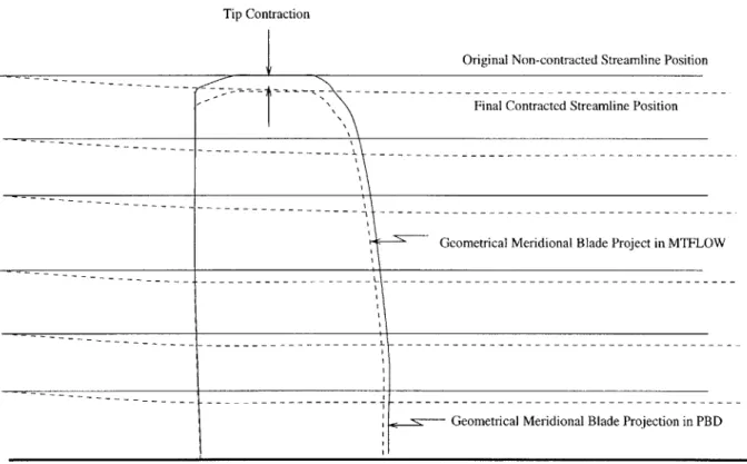
3-2
Streamline contraction due to the presence of the propeller. . . . . .
3-3 Use of swirl elongation factor to counter streamtube contraction
3-4
Open Propeller Coupling procedure between PBD and MTFLOW
3-5
Multiple Blade Row Coupling Flowchart . . . .
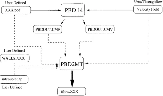
4-1 The interaction and file passing between PBD and PBD2MT
.
. . .
5-1
The interaction and file passing between MTFLOW and BL2BODY
Nominal and Effective inflow velocity comparison . . . .
Nominal and Effective propeller loading calculation . . . .
Circumferential Mean velocity at the blade trailing edge. . . . .
Radial repositioning of streamlines. . . . .
Huang Submarine Body with Stern 1.. . . . .
Comparison of MTFLOW, RANS, and Experiment Velocity Nominal
IBLT and
}1h
power law velocity profile prediction Huang Body 1
Wake Profiles
6-8 Comparison of Swafford Profile and
}I'
Power Law Boundary Layer Velocity Profiles 6-9 Huang Body 1 Stern Profile with Propeller 4577 . . . . 6-10 Propeller 4119 in ITTC Configuration . . . .6-11 comparison of MTFLOW-PBD with P4119 ITTC Test.
. . . .
6-12 MTFLOW Spline interpolation problem view. . . . . 7-1 The geometry of the ducted fan system. . . . . 7-2 The flow grid used within MTFLOW. The long downstream extent is required by
PBD to grow the trailing wake system. The upstream length of the domain is set by the requirement that the inviscid streamlines correctly match the constant inflow assum ption . . . . . 7-3 Radial blade used to start the design process. . . . .
7-4
Re-analysis by PBD14.4 of PBD14.2 blade. . . . .
7-5 These two plots show the final MTFLOW inviscid solution streamlines. The plot on the right is a blow-up of the propeller tip region. Notice that the propeller leading edge tip operates in the extremely accelerated flow round the duct lip. This is a purely inviscid flow effect. . . . . 7-6 As the blade passes through a region of inflow with reduced velocity, the velocity
triangle clearly shows the accompanying increase in angle of attack. . . . . . . . . 1 3
. . . .
1 5
. . . .
1 7
22 24 2629
30
3132
35
40
6-1
6-2
6-3
6-4
6-5
6-6
6-7
7-7 The final fan designs for the back skew, no skew, and forward skew fans. The small plot to the right of the fan shows the distribution of pitch(phi) and skew angle over
the radius of the blade. . . . . 65
7-8 The rake and max section camber for the final fan designs. Notice how the changes in section pitch
(i.e.,
changes in local angle of attack) are accompanied by an offsetting change in section max camber. . . . . 667-9 Comparison of design and analysis blade results. . . . . 67
D-1 Flowfield with spline interpolation problems. . . . . 81
List of Tables
1.1 Outputs from a lifting line analysis. . . . . 14
1.2 Outputs from a lifting surface analysis. . . . . 16
3.1
FORTRAN Coupling Codes.
. . . .
25
4.1 PBD2MT required input files . . . . 34
4.2 PBD2MT Output Files
. . . .
35
5.1 BL2BODY required input files. . . . . 39
5.2
BL2BODY Output Files. . . . .
40
6.1 Validation of coupling technique. . . . . 44
6.2 Boundary layer velocity profile validation tests. . . . . 48
6.3 Huang Body 1 with Propeller 4557: experimental and numerical results. . . . . 54
6.4 Experimental and numerical propeller curve test results for 4119. . . . . 56
7.1 Fan Design Operating Parameters. . . . . 59
B.1 Changes to mtset.f . . . . 73
Symbology
A stream tube cross sectional area
A1, A2 area vector normal to streatube volume along streamtube
B number of blades
B- B+ area vector normal to streatube volume normal to streamtube
H Boundary Layer shape parameter
M mach number
n
Surface normal vectorn propeller rotation rate (rps)
P Pressure
Q
mass flow rater
local radius from centerlinerc meridional radius of curvature of streamtube
RT Total resistance
Reo Boundary Layer momentum thickness-based
Reynold's number
s
unit vector in direction of vmT Barehull resistance
TO circumferential blade thickness
Ue boundary layer edge velocity Xeff Effective Inflow Velocity
Vinduced Induced Inflow Velocity
Vnoninal Nominal Inflow Velocity Vtotal Total Inflow Velocity
, Radial component of meridional velocity V, Axial component of meridional velocity
V Meridional tangential velocity
fO*
Circumferential mean induced tangential velocityVm meridional velocity
VO tangential (swirl) velocity
WT Taylor wake fraction
WN Nominal volumetric wake fraction
Z number of propeller blades
boundary layer thickness
boundary layer displacement thickness
AS added entropy
AW work addition
'YB bound vorticity
IF blade circulation
Q blade rotation rate
p local cell density
[I streamtube normal pressure
0
boundary layer momentum thicknesskinematic viscosity Gradient Operator
S Boundary Layer thickness
6* Boundary Layer displacement thickness
p density
K Radius of curvature of a streamtube
f Circulation
FB
Bound circulation0
Boundary Layer momentum thicknessRotation rate vorticity
Chapter 1
This Thesis in the Propeller
Design Process
A propeller which operates in the shear flow found near the aft end of marine vehicles experiences an intimate coupling between the propeller's induced velocity field and the rotational inflow. The presence of the propeller's induced velocity field causes the inflow to accelerate, which redistributes the vorticity present in the inflow
[14].
This redistribution causes a change in the total inflow velocity to the propeller. Because the propeller now experiences a different inflow, the propeller induced velocity field is altered. Thus, there is an intimate coupling between the vorticity present in the fluid inflow and the propeller-generated induced velocity field. To design more efficient, and more complex, propulsor geometries, it is necessary to accurately account for this physical interaction phenomena.A potential, vortex lattice lifting surface propeller blade design code such as Kerwin's Propeller Blade Design
(PBD)
code is incapable of analytically representing the vortical interaction between the induced velocity field and the rotational inflow. An additional difficulty is encountered as downstream blade elements, which would be present in a multi-component propulsor, pass through the singularity wake sheets shed by upstream components. For these reasons, the propeller blade design code should be coupled with a throughflow fluid solver which is capable of modelling vorticity transport.This thesis focuses on coupling a propeller blade design code developed at MIT by Kerwin [5] with an axisymmetric, multi-element throughflow code, developed at MIT by Drela
[3].
Drela's throughflow solver uses an integral boundary layer method to solve for the boundary layer flow, and a streamline curvature formulation to solve for the inviscid, outer flow. The main advantage of the streamline curvature throughflow code is an order of magnitude reduction in computation time compared with the RANS coupling methodology [14].1.1
Fluid Velocity Terminology
Before proceeding further, it is necassary to first clear up what the propeller designer means when talking about fluid velocities. The nominal inflow is the fluid velocity in the region of the propeller with the propeller not operating. The total inflow is the fluid velocity with the propeller operating. The total inflow velocity is composed of an induced velocity, which is induced by the presence of the propeller blade and trailing wake singularity distributions, and an effective inflow.
Vtotal _ Vinduced +
Ve ifectiv
e (1.1) Figure 1-1 graphically shows the relative magnitudes and directions of the total, induced, and effective inflow velocities for a typical propeller.While the nominal inflow is the inflow field when there is no propeller present, it is not equal to the effective inflow. This is due to the aforementioned interaction effects between the propeller
Total Inflow Induced Velocities Effective Inflow
Figure 1-1: The total, induced, and effective inflow velocity fields generated by Propeller 4119,
J=0.833, in inviscid flow.
vortex lattice and the vorticity in the inflow. This can be seen from the definition of the vorticity vector.
= Vx V
(1.2)
A non-radially-uniform meridional inflow suggests the presence of a tangential component of vortic-ity.
(1.3)
Dx
or
The tangential vorticity can be thought of as a ring which circumscribes the propeller shaft [181. The propeller induced velocity causes a contraction of the tangential vorticity ring. As this ring contracts, Kelvin's thereom requires that the strength of the vorticity remain constant. Therefore, from equation (1.3), it is evident there is a change in - to counteract the change in '. If there were no tangential vorticity present in the inflow, though, the nominal and effective inflows are exactly equal. This fact is used later to validate the coupling methodology in this thesis.
1.2
Effective Inflow
All propeller design and analysis takes place in the effective inflow. Recall that the effective inflow is the total inflow with the effects of the propeller
(i.e.,
the propeller induced velocity component) removed. The effective inflow is a non-physical flow field. It can not be measured in a water tunnel or behind a ship in operation. And, yet, determining the effective velocity field is critical to the success of the propeller design process.Historically, to determine the effective inflow velocity, a model of the ship is constructed, and velocity profile surveys are taken in the propeller disk plane of the unappended model. This is the nominal inflow. The effective inflow velocity is taken as a fraction of the nominal inflow.
- 1
-
WrVef f =
(1-W
)
fnom (1.4) As shown above, though, this linear scaling across all radii means that in the hub region, where the boundary layer dominates the inviscid flow, the velocities are too high, and the velocities over the rest of the blade span are too low. In fact, this method produces the correct velocity at only one radius along the propeller span!A more modern method is to computationally compute the flow in the region of the propeller by
solving the equations of fluid motion, accounting for the presence of the propeller. Thus, the exact total inflow velocity is known at every radii across the propeller span. Once the induced velocity is
subtracted from the total inflow velocity, the effective inflow is known.
Besides the effective inflow velocity, the propulsor designer also requires an accurate knowledge of the thrust power which must be generated by the propulsor at the design speed.
IKT, KQ, 17
Propeller Diameter Spanwise Circulation, IF(r) Propeller RPM
Cavitation Index
o-Table 1.1: Outputs from a lifting line analysis.
1.3
The Coupled Hull Flow Resistance Problem
To accurately design a propeller requires an accurate knowledge of the ship's resistance. The in-creased fluid velocity along the stern of the vessel due to the presence of the operating propeller causes an increase in drag since there is more incomplete pressure recovery. The vortical interaction also wreaks havoc upon the traditional tow tank resistance calculation, since, for vessels with high aft prismatic coefficients, the presence of the propeller can inhibit boundary layer separation.
Historically, the values for the resistance of the ship with and without a propeller operating are related through the thrust deduction coefficient.
RT = (1 - t) T (1.5)
Modern computation techniques which model the interaction of the propeller and the fluid flow around the hull solve both the effective inflow and thrust deduction problems by nearly exactly solving for the fluid flow over the hull with the propeller operating. In this method, the entire submarine and duct, if present, is modelled in the computer. The shear flow is exactly computed along the body, and the correct propeller interaction effects are also modelled.
Once the effective velocity field is known, and the ship, or submarine, resistance is known, we can get on with the task of designing a propeller.
1.4
Modern Design Techniques
The starting point for the propeller design process is the effective inflow. The designer then uses a lifting line theory to optimize the gross propeller characteristics. In lifting line theory the blades are represented as two dimensional "sticks" of bound vorticity [13]. Refinements upon the basic lifting line model allow for hub and duct modelling, and multiple blade rows [2]. Bowles' advanced lifting line method [2] also allows for the cavitation and strength considerations in his lifting line development. Not included in this analysis are skew and rake effects. The outputs of the lifting line analysis shown in Table 1.1 give the several gross propulsor characteristics.
Once the lifting line analysis is complete, a lifting surface propeller code is used to find the two dimensional blade shapes, pitched about a raked and skewed genarator line, which produce the required circulation F(r). While further discussion of lifting-surface theory is delayed until Section 1.5, there are several key output parameters from lifting surface design.
In the serial progression from lifting line to lifting surface design shown in Figure 1-2, the effective inflow is assumed constant. However, a quick check of the numerically predicted induced velocity components against the empirically assumed induced velocity components (remember, the designer had to scale a physical total inflow to get to the effective inflow by subtracting the induced velocity components) would show that there are differences. This should drive the propeller designer to rederive a new effective inflow and optimize a new propeller. Another tact is to couple the preliminary design tools with a viscous (i.e., able to model the viscosity in the governing fluid equations of motion) or inviscid Euler throughflow solver which can accurately model the effects of the propeller vorticity upon the global flow solution. The requirement for preliminary design, however, is a fast, computationally "cheap" solution to allow proper exploration of the design space. The current RANS coupling is not fast in that sense. As will be shown later, an axisymmetric streamtube solver meets both requirements.
Lifting Line Design Blade Representation Lifting Surface Design Blade Representation
C.)
A
No current couplingCurrent Design
between a lifting line Techniques Iterate
blade design code and A Lifting Surface
I throughflow solvers due
Design Code with
to computational expense RANS-based
of RANS-based solvers. rouhfoser
throughiflow solvers
Numerical Representation of Body and Propeller Forces in Throughflow Fluid Solver
Figure 1-2: The prelimary propeller design process relies upon an assumed effective wake (i.e.,velocity field) as input to a lifting line analysis to optimize the propeller and lifting surface analysis to design the three dimensional blade shapes. There is a limited amount of coupling with throughflow solvers to iterate upon the effective wake.
Performance KT, 10KQ, rl, to check thrust and torque.
Blade Offsets Expressed in the traditional propeller design pa-rameters of rake, skew, pitch, camber, and thick-ness distributions this specifies the geometry of the blade for construction.
Spanwise Circulation The final circulation distribution may not match the original desired circulation distribution due to three dimensional rake and skew effects.
Local Pressure Coefficient This gives and indication of cavitation.
Table 1.2: Outputs from a lifting surface analysis.
1.5
Lifting-Surface Propeller Blade Design and Analysis
In a traditional propeller lifting surface propeller code, a grid lattice is placed on the blade mean camber surface, the hub and duct (if present) and the trailing wake system [15]. Each lattice segment is assigned a strength of vorticity. On the solid body surfaces, such as the blade and hub, a control point is placed near the center of the grid lattice. The strength of each vortex lattice segment is assigned by satisfying the kinematic boundary condition that the flow must be tangent to the propeller, hub, and duct surfaces at every control point.
Mathematically, the propeller problem involves a simple matrix equation. By attacking the geometry of the problem, an influence matrix is formulated which gives the velocity induced by a unit strength of vorticity along every vortex lattice upon every control point - an [INF]luence matrix. When multiplied by the actual vortex segment strengths, the induced velocity at every control point is known.
[INF]
[f]
=Vinduced
(1.6)
/noindent To model the effects of blade thickness, a souce distribution is placed coincident with the blade vortex lattice system.
Next, to satisfy the kinematic boundary condition, the physics of the problem dictate that the component of the induced velocity normal to the blade, when added to the component of the effective inflow velocity normal to the blade must be zero.
[[INF]
[f] + Veff
-h = 0
(1.7)
Equation (1.7) is the heart of the propeller lifting surface code.
A lifting surface propeller code can be used for either the design of a new propeller or an analysis of an exsisting propeller. In the case of a propeller design, a radial loading distribution is prescribed, and a blade shape is found which produces the desired loading by manipulating the geometry of the blades. In blade analysis, the unique strength of the vortex lattices segments is found which satisfies equation (1.7). From equation (1.7) it is seen that an incorrect effective inflow velocity will give either an incorrect blade shape, or an incorrect prediction of blade loading.
The propeller forces resulting from the vorticity and source distributions are calculated from the Kutta-Joukowski and Lagally theorems, respectively. A Lighthill leading edge suction force correction is applied to these forces, and the propeller's sectional drag is calculated either based on strip wise two dimensional empirical drag coefficients, or a stripwise 2-D integral boundary layer calculation.
The propeller blade analysis code used in this study is an extension of a previously reported lifting surface design code [12, 5]. The extensions replace the image hub and duct with vortex lattice
Propeller 4119 Vortex Lattice Representation
Transition Wake
Vortex Lattice
Hub Systemd rniin
Figure 1-3: 3 bladed propeller 4119 on a straight shaft. Notice that the hub discretization extends
upstream of the hub. The inner radius of the transition wake vortex lattice is the innermost hub
streamline.
representations of the hub and duct [14, 17]. The computer representation of the blade and hub
vortex lattice, and transition wake is shown in Figure 1.5.
The end result of the propeller blade analysis routine is the complete circumferential mean
induced velocity over the blade surface. The circulation, FB ,is computed from the circumferential
mean tangential induced velocity by the following relationship which follows from the Euler turbine
equation.
.-27rr V*
F2 () =
r
(1.8)
Equation (1.8) is at the heart of the present coupling technique with the streamline curvature
method. In the streamline curvature method, as in turbomachinery mean line design, the designer
is most interested in determining the amount of turning, or swirl, being applied to the flow through
the action of the blades. Therefore, in the coupling with the streamline curvature method, the swirl
r(AV) is directly calculated by multiplying
V,*
by the local radius r. The use of the swirl velocity
to couple between the propeller code and the throughflow solver is unique to the present research.
In previous coupling methodologies, the propeller is represented as distributed body forces within
the RANS throughflow solver.
1.6
Coupling with a Viscous Througliflow Solver
The major shortcoming of the lifting surface formulation described above is the inability to model
the vorticity interaction. As previsouly mentioned, the propeller induction velocities cause a
redis-tribution of the vorticity present in the inflow. This interaction is critical in the design of modern,
full stern submarines, where the stern prismatic coefficient is so high that the propulsor actually
inhibits separation of the boundary layer.
The second area of propulsor design affected by this shortcoming is in the design of multi-element
propulsors. The problem is that at points where the trailing wake vorticity from the upstream blade
rows intersect the control points of the downstream blades, the mathematics of the problem produces
a singular solution. Multi-element propulsor design is important in the design of modern submarine
propulsors, and in the design of waterjet pumps.
And yet, the lifting surface formulation is unequalled by any other technique in its ability to
rapidly and accurately predict the forces produced by a propeller. But it can not model vorticity
interaction. Modern throughflow solvers, though, can accurately model vorticity interaction, but are
too computationally expensive to model the whole propeller problem in three dimensions. Modelling
the three dimensional propeller blade problem in a fast vortex-lattice lifting-surface code means
that a computationaly axisymmetric "cheap" viscous throughflow solver can be used to solve for the circumferential mean flow over the body.
Past researchers have coupled propeller design codes with axisymmetric RANS throughflow solvers. This method is extremely robust, but also extremely time and computationally inten-sive. Thus, it seems logical to couple the propeller blade design code with a streamline curvature code, because the streamline curvature code runs extremely quickly. A simple test case, such as a three bladed propeller on a straight shaft in inviscid flow, takes around 12 hours to run on a typical work station. More complex cases, such as a submarine propulsor, take on the order of days. As a comparison, it takes less than 15 minutes to run the simple propeller in inviscid flow with the present streamline curvature coupling method. Obviously long computer run times do not leave much time for the engineer to refine and optimize the design since so much time is taken up by the analysis of a single design point. The potential time reduction would seem well worth the effort of incorporating the streamline curvature method into the preliminary design as it would allow for more exploratory design efforts, rather than computational analysis.
Chapter 2
Flow Theory
2.1
Computational Solution to Fluid Flow Problems
The governing equations of motion for any fluid flow are the Navier-Stokes Equation [22], written here in compact vector form.
DiT
1D
=
VP+VV2F+ VH
(2.1)
Dt
p
The solution to Equation (2.1) requires discretization in time and space. To ensure accuracy and stability of the numeric solution, the discretization sizes are directly related to the smallest length and time scales present in the flow. It can be shown that due to the extremely small length and time scales involved in boundary layer flows, a complete, numeric solution to the Navier-Stokes equations would require computational resources far in excess of those available today. Therefore, various levels of approximations are introduced to find solutions to equation (2.1).
To make the Navier-Stokes equation tractable, one fundamental approximation is to ignore the viscous terms. This results in the Euler equations of motion for an inviscid fluid. Hydrodynamicists are able to simplify the problem further by considering the fluid as incompressible. For extremely simple flow cases, there exist numerous, classical theoretical solutions to the incompressible, inviscid flow equations. The value of these classical results is not to be underestimated in that they provide an irrefutable answer by which numeric solution techniques can be validated.
Solutions to real world flow problems are only possible using numerical schemes. The large success of incompressible, inviscid numeric computer codes shows that even with the inviscid and incompressible approximations, the majority of the physics of the flow is still correctly modelled. There are, however, ways to introduce the effects of the viscosity without the computational expense of solving the fully three dimensional Navier-Stokes equations.
Since viscous effects are mostly confined to a small region of the flow domain, an effective ap-proximation is to use a "divide-and-conquer" strategy. In this technique, an inviscid Euler solver is used to solve the majority of the flow domain, and a boundary layer solver is used to solve for the boundary layer growth along a solid wall. The two codes co-exist by matching the boundary conditions (pressure and velocity) at the interface between the two flow regions. This type of cou-pling is a displacment body type of scheme and is the scheme employed by the numeric codes used in this thesis. The basic idea is to use a fast, inviscid solver to solve for the inviscid flow and a fast boundary layer routine to solve for the the boundary layer flow.
2.1.1
The Boundary Layer Equations
A significant approximation to the full Navier Stokes equation can be made through the application of dimensional analysis [25]. The resulting simplfied equations, usually termed the Thin Shear Layer Equations or the Boundary Layer equations are quite simplified indeed. They are written here with
the Conservation of Mass equation for completeness in the subsequent derivation of the Integral Boundary Layer Equations.
Continuity
O +
=0
(2.2)
&u & &u Ue 9Ue 1 OT
Momentum
&t+ue
Ox+-
p Oy(2.3)
To formulate the so-called integral boundary layer equations, Equation (2.2) is pre-multiplied by the quantity (u - Ue) and subtracted from Equation (2.3) [25]. The resulting equation is then integrated over the domain for the boundary to infinity.
(e -U)dy + u(e - u)dy + - ( -u)dy -Uevw (2.4)
p
o=
9 tx JOO 0 OX 0where T shear stress on the solid boundary tie inviscid edge velocity
u(y)
local velocityvW velocity through the wall, usually termed as wall transpiration
The key at this point is to recognize the definition of the displacement thickness and momentum thickness buried beneath some algebra within Equation (2.4). Recall the following equations are the definitions for the displacement and momentum thicknesses.
Displacement Thickness * = (1 - uL)dy (2.5)
0 Ue
Momentum Thickness
0
=
-(1
--
)dy
(2.6)
Inserting Equations (2.5) and (2.6) into Equation (2.4) gives the common form of the integral boundary layer equations.
r C; 1 t9 dO 1 due v.
(.7
-2 - - -2(eS*) + + (20 + ) I(2.7)
pU2 2 u2
oft
dx ue dx neIgnoring the wall transpiration term, and allowing only steady flows, Equation (2.7) reduces still further.
Cf
=j - + (2 + H)
dO u(2.8)
2 dx
U
dx(2.8)
where H =
j,
momentum shape factorFrom a computation standpoint, Equations (2.7) and (2.8) are superior because they are parabolic in nature and can be solved through a marching routine. That is, starting from a given upstream starting condition, the solution downstream is found by marching downstream. Equation (2.3), on the other hand, is hyperbolic and must be solved globally and, usually, iteratively.
There remains, however, the complication of a closure relation. In equation (2.8) there are more unknowns than equations. Therefore, we must use an auxiliary equation which relates one, or more, of the unknowns to the others. This auxiliary equation is termed a closure relation when applied to boundary layer flows, and is usually based upon a mix of empiricism and physics. The closure relations used within MTFLOW and the PBD-MTFLOW coupling codes are those derived
by Swafford [23].
2.2
Streamline Curvature Method
The streamline curvature method is a powerful method for solving for the inviscid flowfield within a channel or annular passage
[1,
22]. Because this method is inviscid, it must be coupled with a boundary layer routine to solve for the boundary layer flow. The two then must operate in tandem since the boundary layer tends to displace the inviscid streamlines off the body by the displacementthickness, which causes a redistribution of the inviscid streamlines.
The throughflow computer code developed by Drela [3] is based on the conservative formulation of the steady state Euler eqations developed by Drela [4]. This approach is an improvement upon the original Streamline Curvature Method formulation [19]. Section 2.2.1 shows the basics of the streamline curvature method, section 2.2.2 outlines Drela's reformulation of the problem in a finite volume sense, and section 2.2.3 shows the MTFLOW computer code implementation, which makes another intelligent simplification.
The streamline curvature method has been previously applied to hydrodynamic open propulsors
[20].
2.2.1
The Original Streamline Curvature Method
The streamline curvature method is applicable for axisymmetric meridional flow problems. It was first derived to solve internal flow problems. In the original streamline curvature method, the steady-state conservation of momentum equation is formulated which accounts for changes in radial momentum due to meridional curvature, fluid acceleration, and tangential velocity, or swirl, effects [11].
Fluid accelerations in the radial direction are due to 1. Acceleration in the Streamtube Direction.
vm (
)v
as
which has an outward directed radial componentVm (
Ov,
)sin#
as
2. Meridional Curvature of the Streamtube. The centripetal acceleration is 2
Vm
rc
3. Tangential Velocity. A tangential velocity component (i.e., swirl) implies a centripetal accel-eration
2 V
9
r
The streamline curvature method is based upon the solution of the equations of motion along a streamline in steady flow. In a streamline and normal coordinate system
(
s , n) the equations ofmotion are given as the sum of the three acceleration effects cited above[1].
+ pg =
pV.
-- pw
(2.9)
pl Vml
P1,
A l
A2
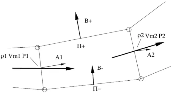
Figure 2-1: Finite Volume geometry and definitions for conservation equations.
+
pg=
pV 2K(2.10)
0on
Notice that the integral of equation (2.9) along the streamline reduces to the usual Bernoulli equation when the rate of rotation, W, is zero.
Equation (2.10) is usually called the radial equilibrium equation. The position of the streamtube boundaries directly gives the fluid radius of curvature term K. This simple ODE is integrated in
the radial direction to derive the mean velocity within the streamtube. The resulting error in the conservation of mass equation is used to drive a relaxation procedure to alter the streamlines towards their correct positions.
The main advantage of the streamline curvature method over traditional time-marching methods is that it is orders of magnitude faster, and hence, applicable to industrial design problems [4]. The main disadvantage of the streamline curvature routine is that the iterative solvers lack numerical stability in regions of supersonic flow, and do not correctly position shocks within the flow. The method of Drela [4] was originally developed to correct this deficiency and correctly treat shocks.
2.2.2
Finite Volume Formulation
Drela's finite volume throughflow method is based on the streamline curvature method. The steady state equations, though, are formulated in a finite volume sense.
The first governing equation is the conservation of mass. Across any two adjoining finite volumes
Conservation of momentum is written as the steady state Euler equation ( Navier Stokes equation sans any viscous terms
).
PiAi
+
(pivmsi - Ai)vmisi + B = P2A 2+
(P2Vm2S2 -A 2)Vm2S2 + H+g+ (2.12)Conservation of energy is formulated in terms of enthalpy.
y
P1 12 _Y
P2 12P + -V =+ Pi -v-2 (2.13)
7-1pi
2 -1 22An additional constraint imposed is that the average pressures on the faces normal to and along the streamtube be equal.
Pi
+ P2=-
f+
+
(2.14)
For the subsonic flow cases which are of interest in marine propeller design, the differential equations form a set of coupled, elliptic, PDE's. The elliptic nature of equations (2.11) through (2.14) requires an iterative relaxation solution procedure, vice a marching solution technique, which would be used in the case of supersonic flow, where the equations are hyperbolic in nature.
The solution is started by specifying an initial gridline distribution. Each gridline pair is treated as a streamtube. Within each streamtube equations (2.11) through (2.14) are solved simultaneously at each streamwise stations using a Newton-Rhapson technique. The solution produces the pressures 11+ and H- on the streamtube walls. By calculating influence coefficients for the effects of streamline curvature and streamtube area on AH, a relaxation equation can be used to update the streamtube positions.
2.2.3
Drela's Throughflow Formulation
Equations (2.11) through (2.14) can be further simplified by forming an explicit scheme that is not differential in nature. The computer code MTFLOW implements such a formulation [3].
The meridional flow speed, vm is obtained from a local streamtube conservation of mass.
Vm = (2.15)
pA(27rr - BTo)
The streamwise momentum equation solved within MTFLOW is of the same form as Equation (2.12).
dP + pvdvm + pvedve + Pd(AS) - pd(AW) = 0 (2.16) The change in work AW enters the formulation through the Euler turbine equation.
AW =
JQd(rve)
(2.17)If entropy losses or enthalpy additions due to heat release occur within the flow domain, they enter the formulation in Equation (2.16). Equation (2.16) is discretized in a finite volume sense as described in section 2.2.2 to preserve shock capturing.
Instead of solving the differential energy equation, which would require large computational times for iterations, MTFLOW solves for the total enthalpy at any location in the flow.
12
ho =
hini + Vini + AH + AW (2.18)The final result is a computationally efficient methodology for solving the inviscid equations of
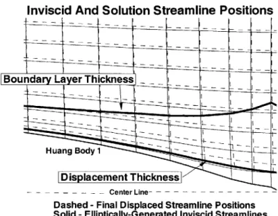
Inviscid And Solution Streamline Positions
|Displacement
Thickness--
--- Center Line--Dashed - Final Displaced Streamline Positions
Solid - Elliptically-Generated Inviscid Streamlines
Figure 2-2: The elliptically-generated streamlines and final streamline positions for the displaced body solution for Huang Submarine Body 1. Notice the overlap area between the displacement thickness and boundary layer thickness.
2.3
IBLT Boundary Layer Representation
While the fluid velocity and pressure gradients along the body are known from the inviscid streamline curvature solution, it remains to solve for the flow within the boundary layer. Drela's formulation of the problem uses an integral boundary layer (IBLT) solver to find the boundary integral quantities knowing the inviscid edge velocity and pressure gradients along the solid boundary. Once the boundary layer flow is known, the body boundary is displaced by the boundary layer displacement thickness, and the inviscid outer flow is resolved. In this manner the boundary layer solution and outer potential flow solution are coupled together.
2.3.1
IBLT Diffculties
The difficulty for the propeller designer with the IBLT is that the IBLT solution gives the integral quantities of the boundary layer, such as momentum thickness and displacement thickness. Because the propeller design code requires the total inflow velocity over the entire surface of the blade, and portions of the blade extend through the boundary layer, the velocity profile of the fluid through the boundary layer has to be reconstructed.
The second difficulty encountered is that the boundary layer displacement thickness, P*, is less than the actual boundary layer thickness,
6.
This is an issue, because the MTFLOW flow solver solution shows high inviscid velocities in the region between 3* and J, while in reality, the slower boundary layer fluid velocity exists.Chapter 3
Coupling PBD and MTFLOW
3.1
Process Overview
The coupling between the streamline curvature code and the propeller blade design code follows that used by Kerwin [14] when he coupled the propeller blade design code with a Reynold's-Averaged Navier-Stokes (RANS) code. The basis of Kerwin's coupling was the use of distributed body forces within the RANS code to represent the presence of the propeller. In the streamline curvature code, the propeller swirl, or angular momentum, is used to represent the presence of the propeller in the
flowfield.
In the present coupled analysis or design, one starts by using the propeller blade design code to predict the loading of the propeller based on an assumed flow field. The blade swirl is then transferred to the streamline curvature code where a throughflow solution is computed. To complete the cycle, a total inflow velocity field is extracted from the throughflow domain and returned to the propeller code. The induced velocities predicted by the previous run of the propeller code are subtracted from the total inflow velocity to arrive at a new effective inflow velocity field. This coupling methodology is shown in Figure 3-1.
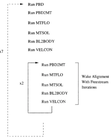
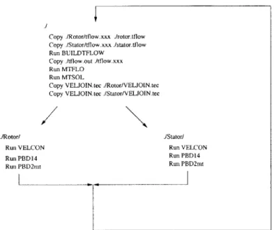
The coupling is automated through the use of small FORTRAN computer codes. The two computer programs shown in Table 3.1 were written to accomplish the coupling. The actual sequence of running computer programs to run a coupled propeller problem is shown in Figure 3-4.
3.2
Obstacles to Coupling
There were several obstacles to overcome in bringing about the PBD-MTFLOW union.
1. Converting propeller blade force quantities into a measure of energy addition to the surrounding fluid consistent with the streamline curvature basis of MTFLOW.
2. Reconstructing a boundary layer velocity profile based upon integral boundary layer quantities.
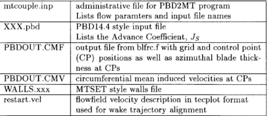
PBD2MT Converts the PBD output circumferential mean induced velocity to swirl. Write out the MTFLO input ascii file containing the swirl, and thickness, if present in the PBD run .
BL2BODY Converts the MTFLOW output boundary layer data into velocity data (i.e., bound-ary layer reconstruction), and writes out velocity data field for use by VELCON. Table 3.1: These two codes are the coupling routines written specifically to couple PBD and MT-FLOW. While no changes were made to any PBD code, the MTFLOW code was altered to output TECPLOT-formatted data files to affect the data transfer.
Propeller Blade Solver
Streamline Curvature to
Vortex Lattice Conversion
o
Boundary Layer Reconstructiono
Velocity Field ExtractionCompute Blade Vorticity
4
Streamline Curvature with
Imposed Swirl
Vortex Lattice Lifting Surface
to
Streamline Curvature Conversion
o
Blade Placement in Flowfieldo
Circulation to Swirl in FlowfieldFigure 3-1: The coupling procedure between the propeller blade design code and the throughflow
solver.
3. Extracting flow field velocities in a manner such that PBD internal data representation did not fail.
4. Allowing for the severe radial redistribution of streamlines in the case of an open propeller. The solutions presented in the following chapters represent my proposed solution to the major obstacles. The final chapters, which present validation and results, show that perhaps there is some merit to these solutions.
3.3
Non-Dimensionalization Issues
The important flow quantities passed between the flow solver and PBD are the flow velocities, the propeller rotation rate, Q, and the propeller swirl, rAV. The flow velocities are used in the blade design code to enforce the kinematic boundary condition on the blade surface. The propeller rotation rate and swirl are used within the throughflow solver to represent the energy imparted to the fluid by the action of the propeller.
3.3.1
Flow Velocities
The magnitude of the velocity is always non-dimensionalized by the inflow speed. This is consistent
between PBD and MTFLOW. Therefore, the velocities do not need to be altered when coupling the two codes, even in the case of contracting or expanding, internal, or ducted flows, or in the case of internal flows where the domain inlet velocity is different from 1.0.
3.3.2
Propeller Swirl
The swirl is used in the Euler turbine equation to calculate the work done on the fluid by the rotor. Because of the length scale inherent in the term, the swirl must be scaled by the proper reference length scale when transposing swirl from PBD into MTFLOW.
3.3.3
Propeller Rotation Rate
Internal to PBD, the non-dimensional advance coefficient, J, is always given as follows.
J =v
(3.1)
nD
1.0 27r
(3.2)
2R
Q
7r J=(3.3)
V, is used to non-dimensionalize the velocities. V, is usually defined as the speed of advance
of the vehicle. In the computation domain where the body is fixed and the flow field has non-zero
velocity at infinity, V, is the value of the upstream velocity at infinity. PBD always assumes that
V,
=
1.0. It is not correct to use
VAto non-dimensionalize velocities to arrive at the advance
coefficient. Notice that the value of the effective inflow velocity in the plane of the propeller swept
volume, commonly called the apparent velocity VA, is not constant throughout the swept volume of
the propeller. Hence, the use of VA would result in ambiguities between experimental and numerical
predictions.
It is common to non-dimensionalize empirical propeller tunnel test data with respect to the
upstream velocity at infinity, V,. In internal flow cases, the upstream velocity at the inlet may not
be equal to 1.0. Yet PBD assumes that V, is 1.0. Hence, if V, is not equal to 1.0, this fact must be
reflected by altering the advance coefficient in PBD. This is the so-called effective advance coefficient.
The use of an effective advance coefficient requires a change in the usually straightforward calculation
of the rotation rate, Q.
Jeff- = 1 0 iniet
(3.4)
nD
Q =r Vniet
(3.5)
Jeff