Disentangling Time-series Spectra with Gaussian Processes: Applications to Radial Velocity Analysis

Disentangling Time-series Spectra with Gaussian

Processes: Applications to Radial Velocity Analysis

The MIT Faculty has made this article openly available.

Please share

how this access benefits you. Your story matters.

Citation

Czekala, Ian et al. “Disentangling Time-Series Spectra with

Gaussian Processes: Applications to Radial Velocity Analysis.” The

Astrophysical Journal 840, 1 (May 2017): 49 © 2017 The American

Astronomical Society

As Published

http://dx.doi.org/10.3847/1538-4357/aa6aab

Publisher

IOP Publishing

Version

Final published version

Citable link

http://hdl.handle.net/1721.1/112099

Terms of Use

Article is made available in accordance with the publisher's

policy and may be subject to US copyright law. Please refer to the

publisher's site for terms of use.

Disentangling Time-series Spectra with Gaussian Processes: Applications to Radial

Velocity Analysis

Ian Czekala1,7, Kaisey S. Mandel2, Sean M. Andrews2, Jason A. Dittmann2, Sujit K. Ghosh3,4, Benjamin T. Montet5,8, and Elisabeth R. Newton6,9

1

Kavli Institute for Particle Astrophysics and Cosmology, Stanford University, Stanford, CA 94305, USA;iczekala@stanford.edu 2

Harvard-Smithsonian Center for Astrophysics, 60 Garden Street, Cambridge, MA 02138, USA 3

Department of Statistics, NC State University, 2311 Stinson Drive, Raleigh, NC 27695, USA 4

Statistical and Applied Mathematics Institute, 19 T.W. Alexander Drive, Research Triangle Park, NC 27709, USA 5

Department of Astronomy and Astrophysics, University of Chicago, 5640 S. Ellis Avenue, Chicago, IL 60637, USA 6

Massachusetts Institute of Technology, Cambridge, MA 02138, USA

Received 2017 February 18; revised 2017 March 24; accepted 2017 March 29; published 2017 May 4

Abstract

Measurements of radial velocity variations from the spectroscopic monitoring of stars and their companions are essential for a broad swath of astrophysics; these measurements provide access to the fundamental physical properties that dictate all phases of stellar evolution and facilitate the quantitative study of planetary systems. The conversion of those measurements into both constraints on the orbital architecture and individual component spectra can be a serious challenge, however, especially for extreme flux ratio systems and observations with relatively low sensitivity. Gaussian processes define sampling distributions of flexible, continuous functions that are well-motivated for modeling stellar spectra, enabling proficient searches for companion lines in time-series spectra. We introduce a new technique for spectral disentangling, where the posterior distributions of the orbital parameters and intrinsic, rest-frame stellar spectra are explored simultaneously without needing to invoke cross-correlation templates. To demonstrate its potential, this technique is deployed on red-optical time-series spectra of the mid-M-dwarf binary LP661-13. We report orbital parameters with improved precision compared to traditional radial velocity analysis and successfully reconstruct the primary and secondary spectra. We discuss potential applications for other stellar and exoplanet radial velocity techniques and extensions to time-variable spectra. The code used in this analysis is freely available as an open-source Python package.

Key words: binaries: spectroscopic – celestial mechanics – stars: fundamental parameters – stars: individual (LP661-13) – techniques: radial velocities – techniques: spectroscopic

1. Introduction

Close binary pairs are the foundation of stellar astrophysics. Measurements of the orbital dynamics in these systems can constrain masses, the fundamental physical parameter in stellar evolution. That information is vital for our understanding of everything from star formation to star death, with wide-reaching implications for issues ranging from molecular cloud collapse and fragmentation, to exoplanets, to cosmology with Type Ia supernovae(Torres et al.2010). A common means of

measuring binary orbital dynamics is through high-resolution spectroscopic radial velocity monitoring. Traditionally, radial velocities for each stellar component are measured by cross-correlating an observed composite spectrum with various Doppler-shifted stellar templates (e.g., TODCOR; Zucker & Mazeh1994). The velocity for each component corresponds to

the Doppler shift, which delivers the maximum cross-correla-tion signal. While cross-correlacross-correla-tion is commonly employed as a workhorse technique, there are several shortcomings to this limited statistical framework. First, in the case of low-signal-to-noise (S/N) data, there can be considerable uncertainty about how well the chosen templates match the true spectra of the stars. Second, in its most straightforward form, cross-correla-tion is unable to meaningfully account for variable spectral lines or uncertain calibration parameters in a principled

probabilistic framework, nuisances which can systematically bias a radial velocity measurement. Lastly, at no point does the cross-correlation framework reconstruct either of the comp-onent spectra, preventing a check of the suitability of the chosen template as well as any detailed photospheric analysis of the stars themselves.

Because the composite spectra of spectroscopic binaries are modulated by a deterministic Doppler shift, it is possible to “disentangle” the intrinsic spectra from multiple observations at different orbital phases. One of thefirst successful attempts was by Bagnuolo & Gies(1991): by viewing the composite spectra

of the double-lined O star AO Cas as various projections of the intrinsic component spectra, they were able to apply iterative tomographic reconstruction techniques and recover the comp-onent spectra. Soon after, Simon & Sturm(1994) developed a

sparse matrix formalism to decompose composite spectra into their components while also optimizing the orbital elements of the binary star. In contrast to traditional radial velocity techniques, spectral disentangling techniques can determine the intrinsic spectra and velocities simultaneously, simplifying the coherent propagation of uncertainties and often resulting in more precise constraints on the orbital parameters(Pavlovski & Hensberge 2010). Spectral decomposition can provide precise

radial velocities even at orbital phases where the lines from both stars overlap, an area of difficulty for cross-correlation techniques. Once disentangled, the component spectra can be further analyzed with conventional spectroscopic techniques to determine the fundamental stellar properties. For example,

The Astrophysical Journal, 840:49 (19pp), 2017 May 1 https://doi.org/10.3847/1538-4357/aa6aab © 2017. The American Astronomical Society. All rights reserved.

7_{KIPAC Postdoctoral Fellow.} 8

NASA Sagan Fellow. 9

Rawls et al. (2016) disentangled the spectra of the double red

giant eclipsing binary KIC9246715 and then used the radiative transfer code MOOG (Sneden 1973) to estimate the effective

temperature, surface gravity, and metallicity for each star. A major advance in spectral disentangling was the realiza-tion that the reconstrucrealiza-tion could be performed quickly in the Fourier domain, thanks to the efficiency of the Fast Fourier Transform (FFT; e.g., KOREL; Hadrava 1995). However, the

FFT introduces some potentially undesirable side effects. Because the FFT treats the spectrum as a continuous, periodic function, it is important to carefully choose “chunks” of the spectrum such that the edges are at the same continuum level, otherwise spectral lines will redshift and blueshift off the edge of the chunk and distort the reconstruction (Ilijic 2004). This

problem can be particularly acute when dealing with a late spectral type star with a high density of spectral lines. While Fourier techniques provide the ability to filter out high-frequency noise (de-noising), they may also have difficulty constraining low-order “continuum”-like features of the spectra, making reconstructed spectra appear wavy (Hadrava 1995). Lastly, the FFT requires that input spectra

be interpolated to a log-λ spaced wavelength grid (a process that introduces correlated noise) and treats the measurement errors as homoscedastic. This means that if the S/N of the spectrum is wavelength-dependent or there happens to be a cosmic-ray hit on a certain region of the detector, there is no straightforward way to adjust the weighting of specific portions of the spectrum.

The flexible probabilistic framework offered by Gaussian processes potentially provides a means to address many of the limitations of traditional orbit measurement and spectral disentangling techniques. In truth, stellar spectra are not actually physically generated from Gaussian processes but are rather the result of nonlinear radiative transfer through complex stellar atmospheres with specific wavelength-dependent ele-mental and molecular opacities. However, for the purposes of inferring intrinsic spectra and stellar radial velocities, simple Gaussian processes offer an attractive framework to model stellar spectra in a purely data-driven manner. Gaussian processes have been used successfully for other time-series applications in astronomy such as, for example, modeling lensed quasar time delays(Hojjati et al.2013; Tak et al.2016),

inferring stellar rotation periods (Angus et al. 2015), and

modeling correlated noise in photometric observations of planet transits and eclipses (Evans et al. 2015; Montet et al.2016).

The content of this paper is as follows. In Section 2, we introduce Gaussian processes and demonstrate how they may be used to model a stellar spectrum. Then, we model a mock double-lined spectroscopic binary—where spectral lines from both components are seen in the composite spectrum—and demonstrate how to simultaneously infer the orbital parameters and the intrinsic spectra of both stars. We also show how the precision of the orbital posteriors and quality of the reconstructed spectra respond to changes in the binary flux ratio and S/N of the data set. In Section 3 we apply our technique to the mid-M binary system LP661-13, recently studied by Dittmann et al. (2017). We demonstrate precise

inference of the orbital parameters and reconstruct the spectra of A and B, which are an excellent match to other mid-M spectral templates. In Section4, we discuss potential extensions of the Gaussian process framework to variable stellar spectra,

telluric line modeling, and precision radial velocity measure-ment for exoplanet detection, and in Section5we conclude the paper.

2. Gaussian Process Spectral Models

In this section, we describe a framework for modeling a stellar spectrum, and sums of stellar spectra, as Gaussian processes. First, we review common notation and theorems for multi-dimensional Gaussian random variables. Second, we explain how a Gaussian process can be used to model a spectrum of a single star that is stationary in time and shows no orbital motion due to the presence of a companion. Third, we introduce a Keplerian orbital model and extend the Gaussian process framework to model the spectral time-series of a double-lined spectroscopic binary. Throughout this section we use archival observations of a single star to simulate observations and demonstrate the development of the framework.

We adopt the notation that

x~ m S( _x, xx) ( )1 signifies that the vector x is drawn from a multi-dimensional Gaussian distribution with a mean vector m and covariance matrixS . The elements ofxx S are the covariances betweenxx

pairwise elements within x and can be specified directly or via a functional prescription. By definition, the likelihood function associated with x is the multi-dimensional Gaussian

2 x x x p , 1 2 det exp 1 2 , x xx N xx x xx x 1 2 T 1 m m m p S S S = _⎜⎛- - - - _⎟ ⎝ ⎞⎠ ( ) ( ∣ ) [( ) ] ( ) ( )

where N is the length of x. For computational reasons, the natural logarithm of the likelihood is frequently used:

x x x p N ln , 1 2 ln det ln 2 . 3 x xx x xx x xx T 1 m m m p S S S = - - -+ + -( ∣ ) [( ) ( ) ] ( )

Following Rasmussen & Williams(2005, Equation(A.5)), we let x and y be jointly Gaussian random vectors drawn from

x y , , 4 x y xx xy yx yy  m_m S_S S_S ~ ⎡ ⎣ ⎤⎦ ⎛ ⎝ ⎜⎜⎡_⎣⎢ ⎤_⎦⎥ ⎡_⎣⎢ ⎤ ⎦ ⎥⎞ ⎠ ⎟⎟ ( )

wherem and_x m are the vector means. The sub-matrices_y Sxx

and Syy are the covariance matrices corresponding to the

elements within x and y, andS encapsulates the covariancesxy

between the elements in x and y;Syx =SxyT. If and only if x

and y are independent willS = . The conditional distribu-xy 0 tion of x given y is also a Gaussian distribution:

x y∣ ~ m( _x+S Sxy -yy1(y-my),Sxx-S S Sxy -yy1 yx). ( )5 These equations are the foundation for constructing the Gaussian process spectra model that follows.

2.1. A Model for Observations of a Single Star For our spectroscopic application, the input vector is the sampled wavelengths of the detector{ }l_{i i}w₌₁and the data vector

is the observed fluxes d{ }i iw=1 d d d d , 6 w w 1 2 1 2 l l l l = =   ⎡ ⎣ ⎢ ⎢ ⎢ ⎢ ⎤ ⎦ ⎥ ⎥ ⎥ ⎥ ⎡ ⎣ ⎢ ⎢ ⎢ ⎢ ⎤ ⎦ ⎥ ⎥ ⎥ ⎥ ( )

where each pixel is indexed by i from 1 to w, the number of pixels in the region of the spectrum under consideration. To illustrate the development of our framework, we use synthetic “mock” data sets generated by the following recipe. First, we create a template by stacking many archival high-resolution observations of the K5 star LkCa14 and smoothing the result with a Gaussian kernel. Then, we sample the spectrum at l and add a known amount of white noise to the data set.

We will model the continuous, intrinsic stellar spectrum as a Gaussian process. A function f l( ), wherel > , is said to0 have a Gaussian process with mean function m l( ) and covariance kernel k(l l¢, ) if for anyfinite collection of inputs 0<l1<l2< ¼ <lw the vector { ( )f l1,f(l2),¼,f(lw)}

has a multivariate Gaussian distribution with mean vector

, , , w

1 2

m l m l ¼ m l

{ ( ) ( ) ( )} and w×w covariance matrix with elements k(l li, j), where i j, =1, 2,¼ , and k is a positive,w

definite kernel function. A single function generated from a Gaussian process is called a realization of the Gaussian process. We consider the continuous, intrinsic stellar spectrum f to be a function generated from the Gaussian process

f( )l ~GP(m l( ),k(l l, ¢)). ( )7 For the purposes of this paper, we will always work with finite-length samplings of the Gaussian process f , either at the detector wavelengths l or finely spaced vectors of our own design. To model a single epoch of a single star, we treat the data d as the sum of a realization f of the Gaussian process with a realization of the noise process N,

d= +f N, ( )8

d~(m S_f, f)+(0,SN), ( )9

d ~ m S( _f, f +SN), (10) where S is a covariance matrix describing the noise of theN

data set. For most spectroscopic observations, this will simply be a diagonal matrix with the Poisson uncertainty for each pixel, unless a particular telescope reduction pipeline provides additional information about inter-pixel covariances. It is assumed that the spectrum has been rectified to have a mean flux of 1, so by design we choose the Gaussian process to have

1

f

m = . In theory, we could allow the mean to vary but in

practice it has little effect on the result as long as a reasonable number (or function of λ) is chosen to be ∼1. The covariance matrixS is populated by evaluating a kernel function betweenf

pairs of input values in l. The choice of the kernel function determines the smoothness of the functions drawn from the Gaussian process. As a distance metric, we compute the velocity distance between two pairs of wavelengths i and j as

r r , c 2 , 11 ij i j i j i j l l l l l l = = -+ ( ) ( )

where c is the speed of light and rij has units of km s-1. A

popular kernel is the squared exponential kernel, which we choose to model our spectra. This kernel specifies the covariance between two pixelsl andi l asj

k r a l a r l , , exp 2 , 12 ij ij ij 2 2 2 = ⎛ -⎝ ⎜⎜ ⎞_⎠⎟⎟ ( ) ( )

where a sets the amplitude of the Gaussian process and has the same units as the rectified flux, and l sets the length scale of the Gaussian process and has units of km s-1_{. In this paper, we} refer to a and l as Gaussian process hyperparameters, and commonly denote these using a.

Now we have fully specified the components of the sampling distribution for the Gaussian process f (Equation (1)), which

can be thought of as a distribution over functions. We use the * subscript to denote realizations of a vector, which is a draw from this distribution:

f_* ~(1,Sf +SN). (13)

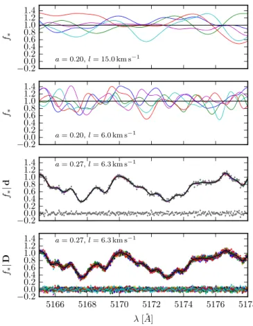
Figure 1.Top two panels: multivariate draws from the prior distribution of functions, given by Equation (13) using a mean of 1 (black line) and the Gaussian process hyperparameters a and l specified in the figure. Completely unconstrained by data, the possible realizations of the Gaussian process span a large range offlux space. As the length scale l is decreased, the correlation length of the realizations also shortens. Third panel: draws of the Gaussian process conditioned on the observed data from a single spectroscopic observation, with the maximum likelihood estimates. Multiple draws from the posterior predictive distribution are shown, with the mean prediction in black and the residuals at the bottom, showing that a Gaussian process can be used to accurately model spectra. Bottom panel: multiple observations of the same star, taken over a series of nights. The sampling density increases dramatically due to the shifting of the barycentric frame.

Several realizations of f* are shown in the top panels of Figure 1, for two different choices of the Gaussian process hyperparameters a and l. While the Gaussian process has a mean of 1, actual realizations of the Gaussian process scatter about the mean. As l decreases, the covariance between distant elements decreases and f* oscillates more rapidly. How does one choose the best values of a and l? Fortunately, the Gaussian process framework provides a natural mechanism to determine the most probable values through the Gaussian process likelihood, given by Equation(2).10In the presence of data (x= , the vector of fluxes), a choice of mean vectord

(m =_x 1), a covariance matrix (Sxx =Sf +SN), and priors on

a and l, the posterior probability distribution is directly specified by the marginal likelihood, Equation (2), which we

can maximize with respect to a and l. Throughout this work we assume flat prior probability distributions for a and l and enforce positivity

p 1 a l, 0

0 else. 14

a =

{

( ) ( )

For some applications it may be worthwhile to explore more sophisticated prior distributions.

With the hyperparameters optimized, we can now make realizations of the Gaussian process conditioned on the data by taking random draws from the posterior predictive distribution (Equation (5)). These draws represent realizations of the

inferred intrinsic stellar spectrum while the scatter in the draws serves to illustrate the uncertainty in our inference and the width of the Gaussian probability distributions at each wavelength. In this application of Equation (5), x=f ;_* y=d; Sxx is filled out by the kernel evaluated over the

prediction wavelengths l_* corresponding to f ;_*

yy f N

S =S +S , whereS is filled out by the kernel evaluatedf

over the wavelengths l corresponding to d; and S is filledxy

out by the kernel evaluated over pairs of wavelengths corresponding to both l_* and l. Random draws of the Gaussian process “snap” to the data (Figure 1, third panel), providing a very flexible mechanism for modeling the continuous stellar spectrum.

Although the Gaussian process achieves promising success in this single-observation application, its real benefit accrues when there are multiple observations of the same star in a time-series. Throughout this paper, we assume that all spectroscopic observations of a target star are acquired by the same telescope, and that the instrument line spread function (LSF) is stable across epochs. For the applications discussed in this paper, these criteria are satisfied by most high-resolution spectro-graphs, such as echelle spectrographs used for radial velocity planet searches. Because convolution is a linear operation, it is reasonable to ignore the effects of the LSF and assume that the intrinsic stellar spectrum we are modeling has already been convolved. For very precise applications (e.g., radial velocity searches for earth-mass planets), variations in the LSF may need to be considered; we discuss this further in Section4.1.

Even though spectrographs may be very stable, such that from epoch to epoch nearly the same wavelengths are sampled by the detector in the topocentric frame, this is not the case in the barycentric frame. Due to the rotation of the earth and its

orbital motion around the Sun, observations of a source that are taken on different days will likely have different relative velocities between the topocentric frame and the barycentric frame, the so-called barycentric correction. This means that at each epoch, the pixels of the detector are sampling slightly different wavelengths of the intrinsic stellar spectrum (broa-dened by the LSF). This barycentric correction can be computed to high accuracy (e.g., Wright & Eastman 2014),

and when all spectra in a time-series are corrected to the barycentric frame we have a very dense(albeit noisy) sampling of the convolved stellar spectrum(see Figure1, bottom panel). We concatenate the W epochs of data and denote new variables

D d d d F f f f , , , 15 W W _W 1 2 1 2 1 2 l l l L = = =    ⎡ ⎣ ⎢ ⎢ ⎢ ⎢ ⎤ ⎦ ⎥ ⎥ ⎥ ⎥ ⎡ ⎣ ⎢ ⎢ ⎢ ⎢ ⎤ ⎦ ⎥ ⎥ ⎥ ⎥ ⎡ ⎣ ⎢ ⎢ ⎢ ⎢ ⎤ ⎦ ⎥ ⎥ ⎥ ⎥ ( ) and D=F+N. (16) The aforementioned covariance matrices are generated from the same kernel as before, with the major difference being that it is now applied to all of the input wavelengths in all epochs, which creates the covariance matrix structure seen in Figure 2. Posterior predictive draws for the multi-epoch Gaussian process are shown in the bottom panel of Figure1.

2.2. A Model for Observations of a Spectroscopic Binary Now, we extend the Gaussian process model to include multiple time-series observations of a spectroscopic binary star system. Typically, labeling a system a spectroscopic binary implies that spectral lines from both stars are seen in the composite spectra; however, we will later show that a simplified version of this framework can also be used to model single-lined spectroscopic binary systems (e.g., stars hosting exoplanets). The orbital motion of each star induces a Doppler shift of the rest-frame stellar spectra, which are then simultaneously observed in composite. If a star is moving with a radial velocity v relative to the barycentric frame, the rest-frame wavelengthsl of the spectrum are shifted to0

v c v

c v 0, 17

l = + l

-( ) ( )

where a positive v denotes a redshift, or increase in the values of the rest-frame wavelengths. The radial velocities of binary stars as a function of time can be fully described by seven parameters q = , Kq A, e, ω, P, T0, γ}, the mass ratio

q=MB MA=KA KB, the velocity semi-amplitude of the primary star, the eccentricity, argument of periastron, orbital period, epoch of periastron, and systemic velocity, respectively (Murray & Correia 2010). The mean anomaly M is given by

Kepler’s equation, M t E t e E t t T P sin 2p 0, 18 = - = -( ) ( ) ( ) ( )

which must be solved tofind the eccentric anomaly E. The true anomaly f is given by f t E t e e E t cos cos 1 cos . 19 = -( ) ( ) ( ) ( ) 10

We will use Equations(2), (4),and (5) throughout this paper and the values ofS ,xx S , andyy S will change depending on the context.xy

Then, the velocity of the primary star as a function of time is vA=KA(cos(w+f t( ))+ecosw)+g (20) and the secondary velocity is

v K

q cos f t ecos . 21 B= - A( (w+ ( )) + w)+g ( ) The resulting spectroscopic binary data set has the same dimensionality as the single star data set, but we now assume that it is produced from the sum of the spectrum of the primary star, denoted by a realization f of a Gaussian process, and the spectrum of the secondary star, denoted by a realization g of an (independent) Gaussian process. The secondary spectrum is produced from a Gaussian process similar to f (e.g., Equation (7)) with the same form of covariance kernel

(Equation (12)). We denote the various components of the

spectroscopic binary data set as

D d d d F f f f G g g g , , , , 22 W W W W 1 2 1 2 1 2 1 2 l l l L = = = =     ⎡ ⎣ ⎢ ⎢ ⎢ ⎢ ⎤ ⎦ ⎥ ⎥ ⎥ ⎥ ⎡ ⎣ ⎢ ⎢ ⎢ ⎢ ⎤ ⎦ ⎥ ⎥ ⎥ ⎥ ⎡ ⎣ ⎢ ⎢ ⎢ ⎢ ⎤ ⎦ ⎥ ⎥ ⎥ ⎥ ⎡ ⎣ ⎢ ⎢ ⎢ ⎢ ⎤ ⎦ ⎥ ⎥ ⎥ ⎥ ( ) D=F+G+N. (23) This spectroscopic binary application can be thought of as modeling the rest-frame spectrum of the primary star (star A), and separately modeling that of the secondary star (star B), while only having access to data sets that represent the sum of the spectra at different orbital phases, all in the presence of noise. We are assuming that the two Gaussian processes are independent from each other and that the Doppler shifts from the orbital motion will allow us to disentangle them. For demonstration purposes, we assume that the orbital parameters

q are known, and therefore we can calculate the radial

velocities of the primary and secondary at all epochs. To fill out the covariance matrix, we must first create new input

vectors corresponding to f and g that relate the observedflux at each epoch to shifted versions of the rest-frame spectra of A and B, , . 24 F A A W A G B B W B 1, 2, , 1, 2, , l l l l l l L = L =   ⎡ ⎣ ⎢ ⎢ ⎢ ⎢ ⎤ ⎦ ⎥ ⎥ ⎥ ⎥ ⎡ ⎣ ⎢ ⎢ ⎢ ⎢ ⎤ ⎦ ⎥ ⎥ ⎥ ⎥ ( )

To produce these vectors, the original sub-components of L are shifted by the predicted radial velocity for each star at each epoch according to Equation(17), such thatL andF L shouldG

correspond to the wavelengths of stars A and B in their respective rest-frames. To be explicit with notation, these input vectors are actually a function of the orbital parameters,L ( )F q

andL ( ).G q

The likelihood function for the sum of f and g is still given by Equation (2), however, the covariance matrix is now a

composite of two covariance matrices plus the noise matrix,

, 25

xx F G N

S =S +S +S ( )

whereS is evaluated usingF L andF S is evaluated usingG LG

with the kernel specified in Equation (12). We show howS isxx

constructed in Figure3. The off-diagonal sub-matrices ofSF

andS denote the cross-epoch covariances of each GaussianG

process. Now that we have completely specified the likelihood function for disentangling the component spectra of a spectro-scopic binary, we relax the assumption that q is fixed. For appropriate values of a and l, the likelihood function will be maximized when q is chosen such that the Keplerian orbit delivers velocity shifts for each epoch that make the cross-matrices consistently describe the rest-frame spectrum of each star.

With the addition of reasonable priors, we can also explore the full posterior distribution of the orbital parameters q and the Gaussian process hyperparameters. Now, we allow separate values of a, l for each spectrum (i.e., a = {af,lf,ag,lg}),

Figure 2. The covariance matrixSxx=SF+SN for multiple epoch observations of the same star. Off-diagonal sub-matrices({l lk, l}, k¹ ) signify thel covariances between nearby wavelengths that are separated in time across epochs. The bands of covariances in the off-diagonal blocks are not exactly centered along the block diagonals because the different barycentric corrections for each epoch mean that the wavelength samplings are different for each epoch. In this representation,S has been multiplied by 50 to better illustrate the structure of the matrix. The elements ofN S have units of flux squared (rectified to 1).xx

since the amplitude and morphology of the spectra of A and B could be significantly different (e.g., an A-type star coupled with an M-type star, or a rapidly rotating primary coupled with a slowly rotating secondary). We can also relax the assumption that the Gaussian process hyperparameters are the same at all wavelengths, for example, to adapt to a star where the spectral line density changes significantly across the observed wave-length range, which we discuss further in 4.

Next, we focus on the formalism necessary to reconstruct the rest-frame spectra of A and B at a vector of rest-frame wavelengths l . The joint probability distribution of the_* (independent) latent Gaussian processes and the data set is given by f g D , 0 0 , 26 f g FG f fF g gG Ff Gg F G N * *  m m m S S S S S S S S S ~ + + ⎡ ⎣ ⎢ ⎢ ⎢ ⎤ ⎦ ⎥ ⎥ ⎥ ⎛ ⎝ ⎜ ⎜ ⎜ ⎡ ⎣ ⎢ ⎢ ⎤ ⎦ ⎥ ⎥ ⎡ ⎣ ⎢ ⎢ ⎢ ⎤ ⎦ ⎥ ⎥ ⎥ ⎞ ⎠ ⎟ ⎟ ⎟ ( ) ( )

whereS andf S are evaluated over pairs of wavelengths ing l_*; F

S andS are evaluated over pairs of wavelengths inG L andF G

L , respectively; andS andfF SgG are evaluated over

cross-pairs of wavelengths in ( *l ,L ) and ( *F l ,L ), respectively.G

The joint posterior predictive distribution is given by

27 f g D D , f g xy yy FG xx xy yy yx 1 1 * *  m m S S m S S S S ~ + - - - -⎡ ⎣ ⎢ ⎢ ⎤ ⎦ ⎥ ⎥ ⎛ ⎝ ⎜⎡_⎣⎢ ⎤_⎦⎥ ⎞ ⎠ ⎟ ( ) ( ) where 0 0 , , . 28 xx f g yy F G N xy fF gG S S S S S S S S S S =⎡ = + + = ⎣ ⎢ ⎤ ⎦ ⎥ ⎡ ⎣ ⎢ ⎤ ⎦ ⎥ ( ) While we will soon demonstrate the many advantages of this Gaussian process formalism for disentangling spectra, it also inherits a few of the limitations common to most disentangling

techniques. First, there is the somewhat obvious limitation that one needs to observe the binary system at multiple orbital phases to obtain different morphologies of composite spectra. If the orbital period of the system is very long, or by chance all observations were obtained at or near the same orbital phase, we would not be able to separate the composite spectra into individual components. Second, because the intrinsic spectra are modeled nonparametrically, without reference to physical models of spectra, reconstruction techniques are unable to say anything about the stellar velocities in an absolute sense. This means that from spectroscopic reconstruction alone we are unable to constrain the systemic velocity of the system,γ, so this parameter remainsfixed to zero in our analysis. Once the spectra are reconstructed, however, γ can be easily recovered by cross-correlation with physical spectral templates. Of related consequence is that the reconstruction technique is only able to constrain the relative velocities of each star from epoch to epoch; it is not possible to measure the velocity of star B relative to star A at any epoch with the reconstruction technique alone. However, this can be later measured easily by correlation with physical spectra models, or if the two stars in question are bound, inferred through their Keplerian orbits.

2.3. Application to Mock Data

To explore the performance of the Gaussian process spectral model, we generate mock spectroscopic binary data sets from a fiducial orbit and assess the accuracy of the recovered stellar spectra and orbital parameters. To generate the data sets, we use segments of real data of the K5 star LkCa14 observed with the CfA/TRES spectrograph on Mt. Hopkins (obtained for a separate purpose under a program with P.I. I. Czekala). Multiple epochs of data were combined and smoothed to create a high S/N template spectrum. We chose two separate regions of this template with an average spectral line density(5235–5285Å for the primary and 6420–6480Å for the secondary) to mimic spectra from two different stars, and then assigned the secondary fluxes to the same wavelength range as the primary. We

Figure 3.For multiple observations of a spectroscopic binary, the structure ofS changes to include the addition ofxx S . Now, there are separate input wavelengthG vectors for each matrix, created by Doppler-shifting the original wavelength vectors to the rest-frame velocities of each star at that epoch. In thisfigure, the covariance kernel for the B star is arbitrarily chosen to be 75% of the amplitude and length scale for that of A(i.e., ag=0.75af, lg=0.75lf).

assume a fiducial binary orbit with q ={KA=5.0 km s-1, q=0.2, e=0.2, ω=10°.0, P=10.0 days, T0=0.0 JD, g = 5.0 km s-1_{}, sampled at 10 epochs over the course of a∼25 day} period (see Figure 4, left panel). To generate a composite spectrum for a single epoch, wefirst Doppler shift each template by its calculated radial velocity, interpolate the secondary spectrum to the same wavelength vector as the primary, multiply each component spectrum by its chosen fractionalflux contribution, truncate each template to the range 5265–5275Å, sum the spectra, and then add random Gaussian noise according to a chosen S/N ratio. This process is illustrated for the first three epochs in the left panel of Figure5. While this mock data set is a small fraction( 1 500< ) of the temporal and wavelength coverage of a typical radial velocity data set, it will serve to illustrate the salient characteristics of our technique in a compact and expedient manner.

Wefirst assess the performance of the technique on a mock data set constructed with moderate flux ratio components and medium-high S/N “observations” ( f f_{B A} =0.2, S/N=60 per resolution element; line spread function FWHM=2.5 pixels), and then explore the robustness of the technique as these quantities are varied to more extreme values. The posterior distribution of the orbital parameters and Gaussian process hyperparameters is

D D

p(q a, ∣ )µp( ∣q a, )p(q a, ), (29) where p( ∣D q a, ) is given by Equation (2) and the prior

p(q a, )=p( ) ( )a p q (30) is the product of Equation (14) and the prior on the orbital

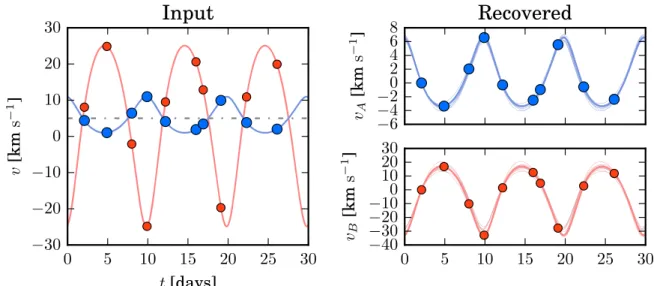
parameters p q( ), which is also flat. The posterior is explored using a simple implementation of Metropolis–Hastings Markov Chain Monte Carlo (MCMC). The inferred family of orbits is shown in the right panel of Figure 4, and these demonstrate good agreement with the input radial velocities. Several draws of reconstructed component spectra and the predicted compo-site spectrum are shown in the right panel of Figure 5. To explore the full distribution of inferred component spectra, we sample from the posterior predictive distribution of the spectra, marginalized over the orbital parameters and Gaussian process

hyperparameters,

f g D f g D

p , p , , , p , d d , 31

* * =

ò

( ∣ ) ( ∣ ) ( ) ( )

where the integration has been performed numerically by the MCMC algorithm. To generate a sample of the reconstructed spectra, we first randomly draw orbital parameters and Gaussian process hyperparameters from the posterior distribu-tion, then draw a sample from the Gaussian process posterior predictive distribution(Equation (27)).

A common limitation of most spectral disentangling techniques is the inability to constrain the continuum level of each star without comparison to a physical model, which our technique suffers from as well. This means that while the relative amplitudes of the variation in each spectrum are well-constrained, there is no knowledge about which star is brighter, i.e., there is a degeneracy between a very luminous companion star with shallow lines and a very faint companion with very deep spectral lines (Bagnuolo et al. 1992). As with the γ

degeneracy, theflux ratio degeneracy can be easily broken by later comparison with aflux-calibrated, physical stellar model (Pavlovski & Hensberge 2010). In the right columns of

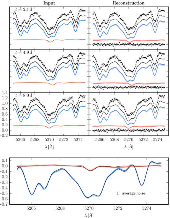
Figure5, we have vertically offset each recovered spectrum by an arbitrary constant to look similar to the left panels, which has the potential to be misleading. Therefore, in the bottom panel of Figure 5, we show the draws of the reconstructed spectra from mean zero Gaussian processes(m_f =m_g =0) to emphasize that they contain no information about the continuum level. Rather, the input spectra have been subtracted by an arbitrary constant to match the level of the reconstructed spectra. The reconstructed spectra do an excellent job of reproducing the shape of the input spectra to a precision that far surpasses the average pixel noise of the mock data set. Interestingly, there is a somewhat appreciable scatter in the vertical offset level of the Gaussian process draws. This is because f* and g* are drawn from a joint posterior predictive distribution, while only their sum is constrained by the data, allowing the mean levels to trade off somewhat (i.e., if a primary draw is slightly higher, then the secondary draw is slightly lower).

Figure 4.Left: thefiducial orbit for a mock double-lined spectroscopic binary (blue=primary, red=secondary), showing the 10 epochs at which the orbit is sampled. Right: the recovered orbits for the primary and secondary stars using the fB fA =0.2, S/N=60 mock data set. Because the spectral disentangling routines are unable to constrainγ, the recovered orbits are plotted relative to the velocity of that star at the first observational epoch.

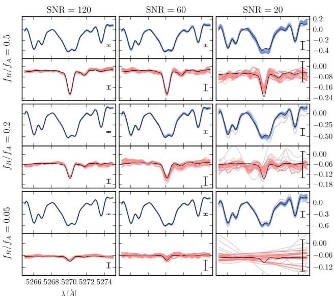
Next, we pursue a grid of tests to explore the performance of the Gaussian process model on mock data with a range offlux ratios f_B f_A = {0.05, 0.2, 0.5} and S/N ={20, 60, 120}. The results of the reconstruction are shown in Figure6, and a visual representation of the one-dimensional marginal posterior distributions is shown in Figure 7. Because of the aforemen-tioned flux ratio ambiguity, we additionally describe our suite of mock data by the standard deviation of the flux of each

spectrum (s andA s ), which is an invariant quantity asB concerns the performance of the technique.

For some binary systems(e.g., eclipsing systems), it may be possible to precisely constrain the orbital parameters via alternate means (e.g., photometric eclipses) to a higher precision than is otherwise possible with a noisy and/or extreme flux ratio spectroscopic data set alone. Therefore in Figure6 we show draws of the inferred spectra marginalized

Figure 5.Left column: to generate a mock observation, the primary(blue) and secondary (red) spectra are Doppler-shifted according to the radial velocities calculated from thefiducial orbit, summed to generate the composite spectra (black), and then noise is added. The resulting data set is shown vertically offset for clarity (black points with error bars). The full mock data set consists of 10 observations of a f f_{B A} =0.2binary with S/N=60. Right column: the distribution of the inferred spectra, sampled from the posterior predictive distributions marginalized over the orbital parameters and Gaussian process hyperparameters(Equation (31)). The primary and secondary component spectra have been offset by arbitraryflux constants, chosen to correspond to the input flux levels for aesthetic purposes. Bottom: the input spectra(black) compared against the draws of reconstructed spectra. In this panel, the reconstructed spectra are drawn from a mean zero Gaussian process (mf =mg= ) to emphasize that our technique cannot constrain the relative flux level of the components, and so the input spectra have been shifted vertically to0 match the level of the reconstructed spectra. Because the reconstruction inference uses multiple epochs of data, we recover the spectra to a significantly higher precision than the average noise in the composite data set.

over the full orbital and Gaussian process hyperparameters (pale gray lines, background) as well as the inferred spectra extracted at the fiducial orbital values but varied over the hyperparameters(hued lines, foreground). The input spectra are shown in black, vertically offset by an arbitrary constant to match the Gaussian process draws as before. To reduce the aforementioned vertical scatter of random draws in this plot, we pin the flux level of primary spectrum to be zero at

5268

l = Å. The average noise per pixel in the data set is shown by an error bar in the right of each panel.

Unsurprisingly, the reconstruction technique performs best for high S/N data sets with moderate (near-equal) flux ratios. The primary spectrum is always accurately inferred across our grid of tests. More importantly, the technique can infer secondary spectra for moderately high flux ratios with very noisy data ( f f_{B A} =0.2, S/N=20) and extreme flux ratios with moderate quality data ( f f_{B A} =0.05, S/N=60), albeit with substantial uncertainty. The inferred values of af and ag approximate the

values ofs andA s , while lB fand lgare a crude measure of the

average width of the spectroscopic lines. For the noisiest, most extremeflux ratio test ( f f_{B A} =0.05, S/N=20), the secondary Gaussian process is unable to constrain the shape of the

secondary other than showing that the amplitude of its variations must be below a certain level(see Figure7). In this situation,

there also emerges a degenerate solution with large agand lg: the

data spectrum is dominated by the primary star modulo the addition of an approximately flat continuum. This degenerate solution could be avoided by the addition of a prior that favors smaller lgat the expected width of the secondary lines. Overall,

the results from this grid of tests are extremely encouraging and demonstrate that the Gaussian process framework is able to accurately infer composite spectra to a precision far exceeding the average noise per pixel in a spectroscopic data set. It is important to emphasize that in these tests we have only been using a single 10 Å chunk of the spectrum; any analyses incorporating a wider swath of spectrum will potentially be much more sensitive.

2.4. Single-lined Spectroscopic Binaries and Exoplanet Search In the limiting case that the flux of the secondary becomes negligible, the system reverts to a single-lined spectroscopic binary and any constraint on the mass ratio (q) vanishes, leaving onlyfive orbital parameters. If there is a strong belief that light from the primary component dominates the composite

Figure 6.Inferred spectra for mock spectroscopic binaries over a grid of S/N and flux ratios, where the average noise per pixel is marked on the right of each panel. Note that the vertical scale is different in each row. In each panel, gray lines(background; wider scatter) represent realizations of spectra marginalized over the full orbital posterior. Hued lines(foreground; tighter scatter) represent realizations of spectra generated with the orbital parameters fixed to the fiducial values (if they were known from external orbital constraints).

Figure 7.Marginal posteriors for the orbital parameters and hyperparameters corresponding to the mock data sets within the test grid. The horizontal blue lines mark thefiducial parameter values, and the violin-shaped plots denote the one-dimensional marginalized posteriors. The width of the posterior represents the probability density(the widest location of the posterior denotes the most probable parameter value), and posteriors that extend off the range of the plot are generally unconstrained over allowable parameter space.

spectrum, then one could save computational time and explore a lower-dimensional parameter space with S = .G 011 How-ever, if there are indeed unrecognized signatures of the secondary in the composite data set, a constrained single-lined spectroscopic model will deliver biased orbital parameters. When using the full complement of binary orbital parameters, the Gaussian process framework provides the ability to place constraints on the relativeflux ratio of an unknown companion in a probabilistic setting. While other search techniques rely upon the cross-correlation and subtraction of a presumed template (e.g., Gullikson et al. 2015), the Gaussian process

framework provides a sensitive, model-free mechanism to detect or place limits on faint spectroscopic lines from a companion star. Of course, secondary contamination is much less an issue in the case of radial velocity measurements of exoplanetary systems around single stars. While any constraints on the nature of the secondary spectrum might be meaningless, such a Gaussian process technique could be used to infer precision radial velocities for planet searches. If a statistically significant non-zero semi-amplitude (KA) and orbital period (P)

were found for the primary star, this would signal the existence of an orbiting exoplanet. The framework could be used to simply infer a high-fidelity template of the primary star, which could be used for analysis of fundamental stellar parameters (i.e., effective temperature, surface gravity, and metallicity) or as a template for traditional cross-correlation radial velocity measurements.

In the development of this framework, we have assumed that the intrinsic spectrum of the star is constant with time, an assumption also made by planet search pipelines using the standard cross-correlation technique. However, subtle changes in the spectrum due to starspots can bias the inferred radial velocity at the level of_{D ~}v 10 m s-1_{(Dumusque et al.2011),} dwarfing the operating precision of state of the art spectro-graphs ( v_{D »}1 m s ;-1 _{Fischer et al. 2016). In the Gaussian} process framework, the effects of starspots could be minimized by incorporating an additional time-covariance that allows for flexibility in the exact shape of the spectrum. Such an extension would be especially useful when simultaneous time-series photometric observations bracket the spectroscopic observa-tions. Measurements of starspot modulation could be used to predict the changes in the spectral line profiles, as is currently done in advanced radial velocity analyses (e.g., Haywood et al. 2014). We further explore the consequences of time

variability in Section 4.2.

3. Results: Application to the Mid-M-Dwarf Binary LP661-13

3.1. The LP661-13 Data Set and Traditional Orbit Analysis As part of the MEarth-South survey (Irwin et al. 2015),

Dittmann et al. (2017) recently discovered the mid-M-dwarf

LP661-13 to be a short-period eclipsing binary. Subsequent photometric and radial velocity follow-up over two observing seasons constrained the system period to be P=4.7043512-+0.00000100.0000013days, the primary component mass and radius to be MA=0.307950.00084M and RA=0.32260.0033R, the secondary component mass

and radius to be MB=0.194000.00034M and RB=0.21740.0023R, and the distance to be 24.9 1.3 pc. Given the lack of strong X-ray emission and the absence of lithium in the spectra, LP661-13 is likely a field-age system. At these masses, both stars are fully convective (M<0.35M; Chabrier & Baraffe 1997). Such a system provides an interesting application for our spectroscopic disentangling technique because the orbital parameters are known to high accuracy due to the eclipsing nature of the system. Moreover, in contrast to solar-type stars, M-dwarfs currently lack high-accuracy synthetic spectral models (e.g., Mann et al. 2013), making the nonparametric, data-driven

Gaussian process approach particularly appealing. For the purposes of demonstrating the disentangling framework, we ignore any eclipse constraints and utilize only the spectroscopic data set in Dittmann et al. (2017). Later, we utilize the

additional constraints from the eclipses to discuss the fundamental properties of LP661-13 A and B, in particular the stellar radii.

The spectroscopic data set consists of 14 epochs (1 hr integration each, except for one 40 minute epoch) taken over the course of 2014 February to 2015 January with the Tillinghast Reflector Echelle Spectrograph (TRES; R=l D =l 44,000) on the 1.5 m Tillinghast reflector at the Fred Lawrence Whipple Observatory on Mt. Hopkins, in Arizona. The data were reduced by the standard TRES pipeline (Buchhave et al. 2010), and placed in the solar system

barycentric frame. At red wavelengths, the S/N of the spectra ranges from 20 to 60 per resolution element, with a median value of 43. To determine radial velocities with TODCOR (Zucker & Mazeh1994), Dittmann et al. (2017) also obtained

high S/N observations of the following mid-M template stars from Kirkpatrick et al. (1991): Gl273 (M3.5), Gl699

(Barnard’s star; M4), Gl83.1 (M4.5), and Gl406 (M6), which we later use for comparison with the disentangled spectra of LP661-13A and B. Dittmann et al. (2017) found the strongest

cross-correlation signal for the LP661-13 wavelengths 7060–7200Å, which contain strong molecular features when using the Gl699 template for both the A and B components in a light-ratio of LB LA=0.4340.025. Because one or both stars may be spotted and the fraction of eclipsed spots is unknown, Dittmann et al. (2017) did not quote a light-ratio

measurement from the eclipse measurements. If one relies upon the derived physical parameters for the system, the temperature scale of Mann et al.(2015), and the Allard et al. (2001) models,

the predicted light-ratio would be LB LA=0.406. Dittmann et al. (2017) omitted the observation on HJD2456743 from

their orbital fit because they were unable to separate the primary and secondary peaks of the CCF, meaning that at this epoch each component had a similar radial velocity. Assuming equal measurement uncertainty for the primary and secondary radial velocities, they calculated a best-fit binary orbit with the 13 epochs of measurements and found the average residuals of the primary and secondary velocities to be 0.05 km s-1_and 0.20 km s-1_{, respectively.}

In order to make a direct comparison with the Gaussian process framework, we re-fit the 13 radial velocities in Dittmann et al. (2017) using the orbital parameterization described in

Section2.2. We adopt 0.05 and 0.20 km s-1_{as the uncertainty} on each radial velocity measurement for the primary and secondary, respectively, and employ a simple _{c likelihood}2 function with flat prior distributions on the orbital parameters.

11

Conversely, this framework could also be used to model single- or double-lined spectroscopic triple systems(via an extension to the orbital model) or even triple-lined spectroscopic triple systems(via an extension to the orbital model and the addition of another Gaussian process component, h).

We explore the seven-dimensional posterior with the emcee implementation (Foreman-Mackey et al. 2013) of the Affine

Invariant Ensemble Sampler (Goodman & Weare 2010). To

assess convergence, we run multiple ensembles of 28 walkers for 10,000 iterations each, starting from different locations in parameter space and burning 5000 iterations worth of samples. We assess convergence by computing the Gelman–Rubin statistic Rˆ (Gelman et al. 2013) for the ensemble of walkers

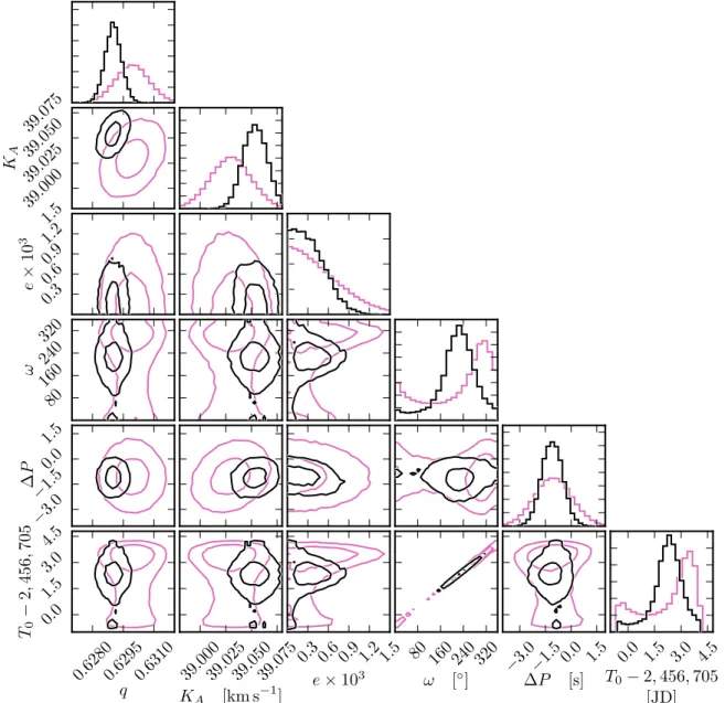
and ensure that Rˆ <1.1. The posteriors are shown in Figure 8

(purple contours) and are in excellent agreement with Dittmann et al. (2017), except for our determination of g =0.025 0.011 km s-1_{, which is discrepant with the value reported by} Dittmann et al.(2017) ( 0.009_{- }0.014 km s-1_{) at the 2s level.} We suspect this may be due to differences in how the radial velocity uncertainties were incorporated in thefitting process. As noted in Dittmann et al.(2017), the orbit is extremely circular,

which leads to the commonw -T0 degeneracy. Therefore, we

also report the summary statistics e sinw = - ( 1 383)´ 10-6 _{and e cosw =(0384)´10}-6_.

In addition to the standard spectral reduction performed by Dittmann et al.(2017), we perform additional processing of the

spectra to facilitate a uniform comparison between objects. Along with the observations of LP661-13 and the 4 aforemen-tioned M-dwarf template stars, we also download an observa-tion of Vega taken on HJD2456740 from the TRES archive (P.I. D. Latham) to use as a reference for telluric line contamination. As part of a typical TRES observational sequence, observations of a continuum source are taken to characterize the echelle blaze function, which has been shown to be very stable with time for most echelle orders. We divide each spectrum by its associated blaze measurement to produce approximatelyflat spectra. This process does not directly lead toflux-calibrated spectra, however, since the absolute bright-ness of the source is not known. Nor does this process necessarily lead to spectra that match the same shape as

flux-Figure 8.The posteriors from the traditional RV analysis(purple, background) and the Gaussian process framework (black, foreground). Contours denote the 1σ and 2σ confidence levels. The γ posterior from the traditional analysis is not shown (_{g =}0.025_0.011 km s-1_{), and the period P is shown relative to the joint} photometric and spectroscopic value reported in Dittmann et al.(2017), P=4.7043512 days. Posteriors from the Gaussian process framework are continued in Figure9.

calibrated spectra, since the spectrum of the continuum source may be significantly different from that of a source originating from above the atmosphere. A TRES calibration program (P.I. I. Czekala) repeatedly observed several spectrophoto-metric standard stars over several months and demonstrated that the TRES intra-order throughput shape is very stable with time. Since the bandpass sensitivity in each order is well-described by a 4th-order Chebyshev polynomial, this means that from night to night the linear and higher-order coefficients varied less than 4%. The inter-order sensitivity is less stable, with nightly scatter typically10%.

Large-scale, sloping features of M-dwarf spectra are important for spectral typing and characterization. Although we do not have observations of spectrophotometric standards contemporaneous with the LP661-13 observations, because the intra-order TRES throughput is stable we can approximate flux-calibrated LP661-13 spectra by applying the sensitivity functions derived from the calibration program, which were measured from a series of observations of the O2 spectro-photometric standard star BD+284211 in 2013 November. Because the edges of the red (l >6800 Å) echelle orders do not have any overlap in wavelength and inter-order flux calibrations are not as stable as intra-order calibrations, we further rectify the spectra so that the medianflux of each order is 1. We also apply a similar transformation to the observa-tionalflux uncertainties, which will be used as an input to the Gaussian process model. The result of this process is spectra whose intra-order shape calibration should be comparable to a bona fide flux-calibration within 4%, but whose inter-order calibration will not be correct. It should be noted that if same-night spectrophotometric flux observations existed, the proper shape of the entire spectrum could be recovered.

3.2. Gaussian Process Inference of Orbital Parameters and the Disentangled Spectra of A and B

We apply our spectroscopic binary Gaussian process frame-work to the pseudo-flux-calibrated data set of LP661-13 in a similar manner as in Section2.3. For computational efficiency, we focus on two high-S/N regions of the spectrum uncontami-nated by telluric lines, 6650–6770Å and 7060–7140Å. Unlike with traditional cross-correlation radial velocity analysis, composite spectra with near-equal component radial velocities still provide useful information in our Gaussian process framework and help constrain the underlying intrinsic comp-onent spectra. Therefore we use all 14 epochs of spectroscopy in our analysis, including the epoch omitted by Dittmann et al. (2017). We divide the data set into 20 chunks of 10 Å each so

that the evaluation of the posterior function can be parallelized across a computer cluster as follows. For each 10 Å chunk, the likelihood function(Equation (2)) is evaluated on an individual

core. A primary process gathers these likelihood evaluations and multiplies them together to form a complete evaluation of the likelihood function. This complete likelihood is multiplied by an evaluation of the prior function (flat with all parameters in this analysis) to yield the posterior evaluation for the full spectral range under consideration. The posterior probability distribution is explored using a simple Metropolis–Hastings MCMC,12 whose jump covariances have been tuned to the structure of the posterior for efficient exploration of the parameter space. We run multiple chains from different starting locations for 40,000

iterations each and assess their convergence with the Gelman– Rubin statistic Rˆ (Gelman et al. 2013), ensuring that Rˆ<1.1. This computation requires about one day on a small computer cluster. The posteriors are shown in Figures 8and 9 (black

contours). We recover similar posteriors as the traditional cross-correlation analysis, and notably several parameters are obtained with higher precision (e.g., q, KA, e, and P). With more

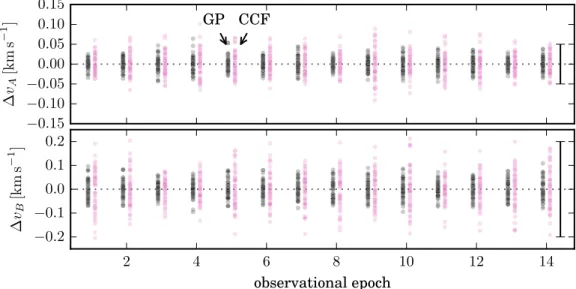
computational resources, a larger spectral range could be included in the analysis and potentially tighten the parameter constraints even further. In Figure 10 we further illustrate the increased precision of the Gaussian process based technique by demonstrating that it delivers a smaller radial velocity scatter at each observational epoch compared to the traditional cross-correlation based technique.

An example of the analysis for a single chunk of the LP661-13 spectrum is shown in Figure11, focusing on a particularly dramatic bandhead for emphasis. The composite data set for each epoch is shown in black, with the corresponding orbital phase labeled in the upper right. Draws of the Gaussian process are generated while varying over random draws of the orbital parameters and hyperparameters from the posterior probability distribution, showing that the distribution of reconstructed component spectra fit well within the noise. As noted in Section 2.3, there is the additional question of choosing the normalization level for each reconstructed spectrum. Thus, in Figure11, we arbitrarily choosem =_f 0.65and m =_g 0.35 to display these spectra(denoted by horizontal dashed lines). We also show the residuals computed from the mean prediction of the composite spectrum at each epoch.

While the exploration of the posterior is performed in 10Å chunks and uses only a subset of the full spectral range, by assuming the inferred orbital parameters and Gaussian process hyperparameters are valid outside of this range one can reconstruct a wide range of component spectra. In Figures12 Figure 9.Posteriors for the Gaussian process hyperparameters, continued from Figure 8. These parameters were inferred simultaneously with the orbital parameters displayed in Figure8but show no significant correlations with any of them. They are displayed here separately for space reasons.

12

Included in theemcee package.

and 13 we show the reconstructed spectra over the full wavelength range 6800–8040Å, which includes many of the notable spectral regions used for classifying M-dwarfs. We also overplot an observation of Vega, a fast rotating A0 star with a near-featureless continuum, in order to highlight regions affected by telluric lines. Any spectral features intrinsic to Vega (e.g., OIλλλ7771) will be broadened by its fast

rotational velocity (vsini₌21.9 km s-1_{; Hill et al. 2004) in} contrast with the narrower telluric lines. In contrast to the carefully chosen narrow range we used for the orbital parameter inference, this expanded region includes numerous telluric absorption lines and night sky emission lines. Because these features are not consistent with the rest-frame of either star A or B, they act to distort the reconstruction process by acting as outlier flux points that cannot be reproduced by the model. In principle, it should be possible to model the effects of telluric lines as an additional Gaussian process since their location is known precisely, although their absorption depth changes from epoch to epoch with airmass and atmospheric conditions. Simultaneous modeling of the telluric features would allow us to access spectral information of the stars in regions that are currently contaminated. We note that other spectral disentangling methods have successfully modeled telluric lines (Hadrava 2006), but we leave a detailed

implementation of these concepts for future work.

Typically, night sky emission lines are subtracted by the TRES reduction pipeline, although in some instances the subtraction is sub-optimal and leaves residualflux. We denote regions affected by poor-night sky line subtraction(Osterbrock et al.1996) with a ◦ symbol and mask these features in the data

set on an epoch-to-epoch basis. Fortunately, because the orbital motion of the binary Doppler shifts the underlying spectra relative to the contaminating night sky line, we are still able to reconstruct the underlying spectrum without significant loss of information.

To properly plot the reconstructed LP661-13A and B spectra (i.e., draws of the mean 0 Gaussian processes conditional on the composite data) in a format suitable for comparison with other rectified observations of mid-M

template stars, we must first renormalize the spectra. Renor-malization refers to the process whereby the spectra are brought to their correct continuum level in the frame of the data with the addition of a constant, and then rectified to a mean of 1 by dividing by that same constant

F F f G G . 32 f g g m m m m = + = + ˆ ˆ _{( )}

For LP661-13A and B, we assume that the mean vectors are simply flat with wavelength, but in principle their relative amplitude could be guided by beliefs about how theflux ratio changes with wavelength, (i.e., m l_f( ), and m l_g( )). An incorrect renormalization will distort the continuum level and the depth of the spectral lines. Because the secondary spectra are intrinsically fainter, they must be scaled by a larger constant to be rectified, which has the effect of making the rectified spectrum appear noisier. We experiment with varying theflux ratio until wefind renormalizations of LP661-13A and B that match the amplitude and slope of the nearby mid-M templates. Wefind that a value ofm m =_{g f} 0.33yields a renormalization that has the spectra of LP661-13A and B closely matching the mid-M templates over the full wavelength range. We note that flux ratios as high as 0.434 (Dittmann et al. 2017) yield

acceptable results over much of the spectral range, however, the contrast of the bandhead at 7090 Å appears too shallow in the secondary spectrum. Frémat et al. (2005) discuss an

alternate renormalization strategy suitable for stars with very deep absorption lines, which must remain positive even in their deep cores, so they set a lower limit on the continuum level of the spectrum. Unfortunately, no such lines exist in the LP661-13 spectra.

3.3. LP661-13A and B in the Mid-M-dwarf Context With the disentangled spectra of LP661-13A and B now known (up to a modest uncertainty in the renormalization factor), we can examine the stars in the context of the other

mid-Figure 10.Relative radial velocity precision of the Gaussian-process-based orbit(GP, left, black points) compared to the traditional cross-correlation-based orbit (CCF, right, purple points) on an epoch-to-epoch basis. For each technique, 50 sets of orbital parameters are drawn from the posterior probability distribution (Figure8), radial velocities are computed for each observational epoch, and then are plotted relative to the mean radial velocity at that epoch. The CCF radial velocity uncertainty measured by Dittmann et al.(2017) is shown by the error bar in the right of each panel. The Gaussian process technique delivers a per-epoch radial velocity scatter that is~50%of that of the traditional CCF technique.

M spectral templates. We have assumed that the flux ratio between A and B is constant across the full wavelength range— given that both stars are evidently very close in spectral type this appears to have been a reasonable decision. Next to LP661-13A and B, we also plot TRES observations of mid-M standard stars (Kirkpatrick et al. 1991) and highlight several spectral regions

commonly used in classification, which generally include molecular features. With low to moderate resolution spectra, the flux within these bands measured relative to a nearby pseudo-continuum region serves as an index for objective spectral typing. Some of the most widely used indices are summarized by Lépine et al. (2013): CaH2, CaH3, and TiO5 Figure 11.Thirteen epochs of composite spectra are shown for a highlighted 10 Å chunk. A 14th epoch at phasef =0.03was omitted from thisfigure for space reasons, since it is the same phase as thefirst plot but has a lower S/N. Ten realizations of the primary and secondary are drawn from the posterior predictive distribution(blue and red, respectively), and residuals are computed from the mean prediction.

(Reid et al. 1995); VO1 (Hawley et al. 2002); and TiO6 and

VO2(Lépine et al.2003). Those most sensitive (i.e., changing

most rapidly) for M3–M6 stars are the TiO5, TiO6, and VO2 indices(Lépine et al.2013).

We would like to directly measure the indices for the disentangled spectra of LP661-13A and B and report an index-based spectral type for these stars. Unfortunately, the format of the TRES echelle spectra complicates a straightforward measurement of these indices, which are measured as the ratio of the average flux in a “numerator” region (marked in Figures 12 and 13) to that of a “denominator” region (not

marked). Unfortunately, for all but one of the indices the numerator and denominator regions fall in different echelle orders, rendering the inadequacies of our pseudo- flux-calibra-tion as a dominant source of systematic error. For the one index (CaH3) that falls entirely within a single order, our measure-ments of the template stars followed the general trend with spectral type but were uniformly 15% larger than those reported in Lépine et al. (2013). We suspect that this

discrepancy is either a remnant of the pseudo-flux calibration process or due to the significantly higher resolution of our instrument, which Lépine et al. (2013) note can bias an index Figure 12.Reconstruction of LP661-13A and B, showing 10 realizations of the spectra (thin, faint lines) overplotted with the mean prediction (thick, hued lines), compared to 4 mid-M spectral templates in black: Gl273 (M3.5), Gl699 (Barnard’s star; M4), Gl83.1 (M4.5), and Gl406 (M6). Common spectral indices used to type M-dwarfs are marked: CaH2, CaH3, TiO-α, and TiO5. A spectrum of Vega is shown on top to highlight areas contaminated by telluric lines. Severely disrupted regions are marked with a gray background.

measurement. Therefore, instead of comparing indices, we directly compare the morphology of the spectra by eye within the noted index regions. We find that LP661-13A and B naturally fall in a sequence of mid-M standards near Gl699 (M4) and Gl83.1 (M4.5), which agrees well with the previously determined composite spectral types of M3.5 (optical; Reid et al.2004) and M4.27 (NIR; Terrien et al.2012).

We emphasize that other than the procedure performed in Equation(32) for LP661-13A and B, no post-processing (e.g.,

continuum or pseudo-continuum normalization) has been applied to any of the spectra presented in Figures 12and 13. If a proper flux-calibration of the data were performed on the raw data and theflux ratio correctly specified, then the inferred shape of the reconstructed spectra would be correct. The ability

of the Gaussian process technique to constrain the low-order shape of inferred spectra avoids a potential downside of Fourier disentangling techniques.

The Gaussian process technique can also disentangle emission lines, and we find that both LP661-13A and B show strong Balmer series emission—in fact, the radial velocity semi-amplitude is large enough such that the emission lines from A and B are completely separated at quadrature. The strong Balmer emission indicates that both stars are magnetically and chromospherically active(Hawley et al.1996; West et al.2011; Lépine et al.2013),

possibly as a result of rapid, synchronous rotation due to tidal locking (Dittmann et al. 2017; Newton et al. 2017). Because

magnetic activity serves to trapflux and inflate stellar radii while decreasing effective temperature (Morales et al. 2009, 2010), it Figure 13.A continuation of Figure12. Regions that were masked due to poor subtraction of night sky emission lines are marked with a◦ symbol. Because these regions are relatively unconstrained by data, the reconstructed spectra revert to draws from the Gaussian process prior.