HAL Id: hal-01075038
https://hal.archives-ouvertes.fr/hal-01075038
Submitted on 16 Oct 2014
HAL is a multi-disciplinary open access
archive for the deposit and dissemination of
sci-entific research documents, whether they are
pub-lished or not. The documents may come from
teaching and research institutions in France or
abroad, or from public or private research centers.
L’archive ouverte pluridisciplinaire HAL, est
destinée au dépôt et à la diffusion de documents
scientifiques de niveau recherche, publiés ou non,
émanant des établissements d’enseignement et de
recherche français ou étrangers, des laboratoires
publics ou privés.
Homography-based Visual Servoing for Autonomous
Underwater Vehicles
Minh-Duc Hua, Guillaume Allibert, Szymon Krupínski, Tarek Hamel
To cite this version:
Minh-Duc Hua, Guillaume Allibert, Szymon Krupínski, Tarek Hamel. Homography-based Visual
Servoing for Autonomous Underwater Vehicles. Proceedings of the 19th IFAC World Congress, 2014,
Aug 2014, Cape Town, South Africa. �10.3182/20140824-6-ZA-1003.01665�. �hal-01075038�
Homography-based Visual Servoing for
Autonomous Underwater Vehicles
Minh-Duc Hua∗Guillaume Allibert∗∗ Szymon Krup´ınski∗∗∗
Tarek Hamel∗∗
∗Institut des Syst`emes Intelligents et de Robotique (ISIR)
UPMC-CNRS, Paris, France (e-mail: [email protected] r)
∗∗I3S UNSA-CRNS, Sophia-Antipolis, France
(e-mails: allibert(thamel)@i3s.unice.f r)
∗∗∗Cybernetix, Marseille, France
(e-mail: [email protected] r)
Abstract: A nonlinear visual servoing approach is proposed for the stabilisation of fully-actuated autonomous underwater vehicles (AUVs) by exploiting the homography matrix between the two images of a planar scene. In a cascade manner, an outer-loop control defines a reference setpoint based on the homography matrix, and an inner-loop control ensures the stabilisation of the setpoint by assigning thrust and torque controls. In contrast with conventional kinematic solution, the proposed controller deals with the high nonlinearity and coupling of the system dynamics and ensures almost-global asymptotical stability. In addition, the interactions of the AUV with the surrounding fluid (e.g., added mass and drag effects) are often difficult to model precisely whereas they may significantly perturb its motion. The proposed controller –augmented with an effective integral action– allows for the compensation of model uncertainties and for robust performance against such perturbations. Simulation results illustrating these properties on a realistic AUV model subject to sea current are reported.
1. INTRODUCTION
The object of the present paper is a class of fully-actuated underwater vehicles whose thrust and torque controls can be assigned independently. While this config-uration is typical for remotely operated vehicles (ROVs), it also exists in some autonomous underwater vehicles (AUVs).Underwater environment gives rise to several con-trol difficulties. For instance, the dynamics of an under-water vehicle is highly nonlinear and characterized by a strong coupling between translational and rotational dynamics, mainly due to added mass effects [Fossen, 2002]. In addition, the key issue related to the control of AUVs is the lack of lightweight and reliable position sensors. A vision system, being lightweight, passive and adaptable, can be used, at least partially, to respond to this challenge. By using a camera as the primary sensor for relative position, the control problem can be cast into Image-Based Visual Servo (IBVS) control problem [Chaumette and Hutchinson, 2006], which opens the possibility to perform autonomous tasks in low-structured environments with no external assistance. Classical visual servo con-trol was developed for serial-link robotic manipulators [Chaumette and Hutchinson, 2006] and more recently for aerial vehicles [Guenard et al., 2008], [Gon¸calves et al., 2009]. In the underwater robotics field few attempts have been made to use vision sensors to perform tasks related to man-made structures such as pipeline following [Rives and Borrelly, 1997, Krupinski et al., 2012] using linear features, or station keeping [Lots et al., 2001] using point
⋆ This work was supported by the French Centre National de la Recherche Scientifique(CNRS) within the PEPS CONGRE project.
features. When the visual target is planar, an IBVS control scheme is proposed in [Benhimane and Malis, 2007] using the homography matrix that encodes transformation in-formation between two images of the same planar target and that can be directly retrieved from the corresponding images. This homography-based visual servoing (HBVS) scheme is a purely kinematic control, initially designed for fully-actuated manipulators. However, its stability and convergence properties are only local and are not provable when the system’s dynamics is taken into account. The HBVS problem has also been investigated for underactu-ated aerial vehicles [Metni et al., 2005], [de Plinval et al., 2013]. In [Metni et al., 2005], additional information such as the orientation measurement of the camera with respect to the target is assumed to be available. In contrast, the HBVS solution proposed in [de Plinval et al., 2013] only makes use of the homography matrix along with gyro-scope’s measurements. However, only local (exponential) stability is proved based on Lyapunov-like analysis. In fact, the consideration of the vehicle’s dynamics within the control design is crucial to obtain provable (strong) stability. These works also show that significant efforts are required in order to eliminate the assumptions concern-ing the precise knowledge of environment geometry. The present study is an alignment with these efforts. Although the AUV system under consideration is fully-actuated, the strongly coupled translational and rotational dynamics represents another challenge. Moreover, in contrast with existing HBVS solutions, an important original outcome of the proposed control approach is related to the obten-tion of almost-global asymptotical stability by means of continuous feedback control.
The paper is organized as follows. Notation, system model-ing and HBVS problem are described in Section 2. Control design is presented in Section 3. In Subsection 3.1, an inner-loop control is proposed for the stabilisation of refer-ence velocity setpoint, based on some modifications of the prior work [Krupinski et al., 2012]. In Subsection 3.2, we present the main result of the paper concerning the design of an outer-loop control directly based on the homogra-phy matrix, with the objective of assigning a reference velocities setpoint for the inner-loop control. Section 4 reports simulation results illustrating the performance of the control approach on a realistic AUV model. Finally, conclusions are given in Section 5.
2. PRELIMINARY MATERIAL 2.1 Notation
The following notation is used (see Fig. 1):
Fig. 1. Notation.
• G and B are the vehicle’s center of mass and center of buoyancy, respectively, m its mass and J0 its inertia
matrix. Let l denote the distance between G and B. • A = {O; −→ea
1, −→ea2, −→ea3} is an inertial frame chosen such
that its −→ea
3–axis points downwards and coincides with
the gravity direction. B = {B; −→eb
1, −→eb2, −→eb3} is a frame
attached to the body whose origin coincides with the vehicle’s center of buoyancy. C = {C; −→ec
1, −→ec2, −→ec3} is a
frame attached to the camera, which is displaced from the origin of B by a vector −−→BC and keeps its base vectors parallel to those of B. Let rC ∈ R3 and rG ∈ R3 denote
the vectors of coordinates expressed in the frame B of−−→BC and−−→BG, respectively.
• The orientation of the body-fixed frame B with respect to (w.r.t.) the inertial frame A is represented by the rotation matrix R ∈ SO(3).
• The position vectors of the origins of the body-fixed frame B and the camera frame C, expressed in the inertial frame A, are denoted as p and pC, respectively. Their
relation is p = pC− RrC.
• The angular velocity vector of the body-fixed frame B relative to the inertial frame A, expressed in the frame B, is denoted as Ω = [ω1, ω2, ω3]⊤ ∈ R3. The translational
velocity vectors of the origins and the frame B and the frame C, expressed in the frame B, are denoted as V ∈ R3
and VC∈ R3, respectively.
• {e1, e2, e3} denotes the canonical basis of R3. I3 is the
identity matrix of R3×3. For all u ∈ R3
, the notation u×
denotes the skew-symmetric matrix associated with the cross product by u, i.e., u×v = u × v, ∀v ∈ R3. The
Euclidean norm in Rn is denoted as | · | and (·)⊤ denotes
the transpose operator.
• satδ(·) ∈ Rn, with δ > 0, is the classical saturation
function defined as satδ(x),x min (1, δ/|x|) , ∀x ∈ Rn.
• satc∆(·) ∈ R3, with some positive diagonal matrix
∆ = diag([δ1, δ2, δ3]), is a saturation function defined as
satc∆(x), [ satδ1(x 1) satδ2(x2) satδ3(x3) ]⊤ , ∀x ∈ R3 . 2.2 System Modeling
Without loss of generality, let us assume that G lies on the −→eb
3–axis and under the center of buoyancy B such
that rG= le3, i.e., bottom-heavy vehicle.
Define W, [V⊤ Ω⊤]⊤∈ R6. When characterized at the
center of buoyancy B, the kinetic energy of the vehicle is given by (see [Leonard, 1997]):
EB= 1 2W ⊤M BW, with MB, [ mI3 −mrG× mrG× J0 ] . According to Kirchhoff and Lamb theory [Lamb, 1932], the kinetic energy of the liquid surrounding the vehicle is given by: EF = 1 2W ⊤M AW, with MA, [ M11A M12A M21A M22A ] ,
where MA ∈ R6×6 is known as the added mass matrix,
which is constant and symmetric. The total kinetic energy of the body-fluid system is ET= EB+EF = W⊤MTW,
where the positive-definite matrix MT is given by:
MT = MB+ MA= [ M D⊤ D J ] , with M, mI3+ M11A, J, J0+ M22A, D, mle3×+ M21A. The matrices M11 A and M 22
A are often referred to as added
mass and added inertia matrices, respectively. One derives the translational and rotational momentums as follows:
P=∂ET
∂V = MV − DΩ, Π=
∂ET
∂Ω = JΩ + DV.
Then, the equations of motion satisfy [Leonard, 1997]: ˙p = RV ˙ R= RΩ× ˙ P= P × Ω + (mg − FB)R⊤e3+ FD+ FC ˙ Π= Π×Ω+P × V+mgle3× R⊤e3+ΓD+ΓC (1a) (1b) (1c) (1d) The term (mg − FB)R⊤e3 is the contribution of both
gravitational and buoyancy forces. The cross term mgle3×
R⊤e3represents the gravitational moment w.r.t. the center
of buoyancy. The expansion of P × V in Eq. (1d) shows that the term (MV) × V should not be neglected in the control design due the added mass effects [Leonard, 1997].
The terms FD and ΓD represent the damping force and
torque due to fluid pressure and viscous drag. Finally, FC ∈ R3 and ΓC ∈ R3 are the force and torque control
vector inputs.
2.3 Homography-based Visual Servo Control Problem The vehicle is assumed to be equipped with a camera, an Inertial Measurement Unit (IMU) and a Doppler velocity log (DVL). The IMU provides the measurements of the angular velocity Ω and the gravitational direction R⊤e
3
(i.e., roll and pitch angles), whereas the DVL measures the translational velocity V.
A reference image of a planar target is taken at some desired pose (i.e., position and orientation). Based on this reference image and the current image, the control objective consists in stabilising the pose of the camera to the desired one. Assume that the camera provides the measurement of the homography matrix H, which contains geometric information about the rotation and translation between two reference frames (see Fig. 1). The homography matrix H is given by [Benhimane and Malis, 2007]:
H= R⊤− (1/d∗)R⊤p
Cn∗⊤, (2)
where d∗ is the distance between the target plane and
the camera optical center, and n∗ = [n∗
1 n∗2 n∗3]⊤ is the
unit vector normal to the target plane expressed in the reference camera frame.
Hypothesis 1. Assume that the reference image is taken when the AUV stays in a horizontal plane. In addition, the inertial frame A are chosen attached to the reference pose of the camera (see Fig. 1).
Hypothesis 2. Assume that a rough knowledge of n∗ is
available such that one can choose a unit vector m∗ ∈ S2
such that n∗⊤m∗> 0.
The control objective can be stated as the stabilisation of H about the identity matrix I3, or equivalently the
stabilisation of (R, pC) about (I3, 0).
3. CONTROL DESIGN
The proposed control approach is split into two cascade parts. The first part –termed inner-loop control– ensures the stabilisation of the translational and angular velocities to a desired setpoint. The second one –termed outer-loop control– is specifically designed from the homography matrix to define the desired velocities setpoint.
3.1 Inner-loop Control
The control objective taken consists in stabilising the AUV’s velocities (V, Ω) about the reference velocities (Vr, Ωr), specified by the outer-loop control. The
ad-ditional objective is the stabilisation of −→eb
3 about −→ea3
or equivalently of Re3 about e3. This objective can be
translated as the stabilisation of the AUV in a horizontal plane. To this purpose, let us define the reference angular velocity Ωras:
Ωr, ω3re3+ kωe3× R⊤e3, (3)
where kω is a positive gain and the third component ω3r
of the reference angular velocity is dynamically assigned by the outer-loop control. The first two components of Ωr
defined by the term kωe3× R⊤e3 are dedicated to the
stabilisation of Re3 about e3. The remaining degree of
freedom ω3r can be independently used for other control
objectives related to the yaw motion. Define the velocity error variables
e
V, V − Vr, Ωe , Ω − Ωr. (4)
Then, the control objective is equivalent to the stabilisa-tion of ( eV, eΩ) about zero.
The inner-loop controller here proposed is reminiscent of the one in [Krupinski et al., 2012], but it is robustified by means of integral corrections. Let zV and zΩ be the
bounded conditional integrators of the linear and angular velocity errors, whose dynamics are given by:
{ ˙zV = −kzVzV+kzVsat δV(z V+ eV/kzV), zV(0) = 0 ˙zΩ= −kzΩzΩ+kzΩsat δΩ(z Ω+ eΩ/kzΩ), zΩ(0) = 0 (5a) (5b) with positive numbers kzV, kzΩ, δV, δΩ. Define the
follow-ing augmented error variables: ¯
V, eV+ kiVzV, Ω¯ , eΩ+ kiΩzΩ, (6)
with positive integral gains kiV and kiΩ. Then, using Eqs.
(1c), (1d), (4), (6), one obtains the following coupled dynamics of ¯Vand ¯Ω: M ˙¯V− D ˙¯Ω= (MV−DΩ)×Ω+(M ¯¯ V−D ¯Ω)×Ωr + (mg−FB)R⊤e3+ FD+ F + FC J ˙¯Ω+ D ˙¯V= (JΩ+DV)×Ω¯ + (MV−DΩ)×V¯ + (J ¯Ω+ D ¯V)×Ωr+(M ¯V−D ¯Ω)×Vr + mgle3× R⊤e3+ ΓD+ Γ + ΓC (7a) (7b) with F and Γ computable by the controller and defined by F,−M ˙Vr+D ˙Ωr+kiVM˙zV−kiΩD˙zΩ+(MVr−DΩr)×Ωr − kiΩ(MV−DΩ)×zΩ− (kiVMzV−kiΩDzΩ)×Ωr Γ,−J ˙Ωr− D ˙Vr+ kiΩJ˙zΩ+ kiVD˙zV + (JΩr+ DVr)×Ωr+ (MVr− DΩr)×Vr − kiΩ(JΩ+DV)×zΩ− kiV(MV−DΩ)×zV − (kiΩJzΩ+ kiVDzV)×Ωr−(kiVMzV−kiΩDzΩ)×Vr
From here, the paper’s first result is proposed.
Proposition 3. Consider the error system (7a)–(7b) and apply the following controller:
FC=−satc∆V(KVV) − (M ¯¯ V)×Ωr+ M ⊤( ¯Ω ×Vr) − ¯Ω× (DΩr) − (mg − FB)R⊤e3− FD− F ΓC=−satc∆Ω(KΩΩ)−(I ¯¯ Ω)×Ωr+(D ¯Ω)×Vr−ΓD−Γ (8)
where KV, KΩ are some positive diagonal gain matrices
and ∆V, ∆Ωare some positive diagonal matrices involved
in the saturation functions. Assume that Vr, Ωrand their
derivative are bounded. Then,
(1) (V, Ω, Re3, zV, zΩ) converges to (Vr, Ωr, ±e3, 0, 0)
for all initial conditions.
(2) The equilibrium (V, Ω, Re3, zV, zΩ) = (Vr, Ωr, e3, 0, 0)
is almost globally asymptotically stable and locally ex-ponentially stable. Conversely, the undesired
equilib-rium (V, Ω, Re3, zV, zΩ)=(Vr, Ωr,−e3,0, 0) is unstable.
The proof is given in Appendix A. The knowledge about the derivative of the reference velocities Vr and Ωr are
necessary to compute the feedback control FC and ΓC. In
the following, we show how this fact influences the HBVS outer-loop control design.
3.2 Outer-loop Control: HBVS Control Design
The outer-loop control design is based directly on the homography matrix H. Control design difficulties lie in the fact that the depth d∗ and the normal vector n∗ involved
in the expression (2) of H are unknown and that this matrix only contains a coupled information of rotation and translation. For instance, let us recall a well-known result proposed in [Benhimane and Malis, 2007]. Let ep, eΘ∈ R3
denote the error vectors defined as:
ep, (I3− H)m∗, eΘ, vex(H⊤− H), (9)
with some arbitrary unit vector m∗ ∈ S2 satisfying
Hypothesis 2. Then, the kinematic control law
with λp, λΘ some positive gains, makes the equilibrium
(R, pC) = (I3, 0) locally asymptotically stable [Benhimane
and Malis, 2007]. A weakness of this kinematic controller is the local basin of attraction of the equilibrium. On the other hand, due to the strongly coupled translational and rotational dynamics, this purely kinematic control ap-proach may fail to guarantee the stability of the controlled system. In the present paper, we aim at working down to the dynamical level with the objective of yielding a controller with a significantly enlarged domain of stability and enhanced robustness.
3.2.1 Reference Translational Velocity Design:
Differen-tiating H given by Eq. (2), one obtains ˙
H= −Ω × H − (1/d∗)VCn∗⊤. (11)
It follows that the derivative of ep defined in (9) satisfies
˙ep= −Ω × (ep− m∗) + a∗VC, a∗, (n∗⊤m∗)/d∗. (12)
For control design insights, let us, for instance, consider the kinematic control design using the camera velocity VC as
control input, with the objective of stabilising ep about
zero globally. In view of Eq. (12), the control difficulty lies in the unknown multiplicative constant a∗. However, we
know that it is positive in view of Hypothesis 2.
Lemma 4. – Kinematic Control – Assume that Ω is bounded for all time and consider the following auxiliary
dynamics: ˙z
p= −Ω × ep, zp(0) = 0 . (13)
Then, the kinematic control law
VC= VCr, −k1ep− Ω × zp (14)
globally asymptotically stabilise ep about zero.
Proof: Using Eqs. (12), (13) and (14), one verifies that ˙ep= −Ω × ep− a∗k1ep− a∗Ω× (zp− z∗p), (15)
with z∗
p , m∗/a∗. Consider the following Lyapunov
func-tion candidate L0 , 1/(2a∗)|ep|2+ 1/2|zp − z∗p| 2
. Using Eqs. (13) and (15), one verifies that the derivative of L0
satisfies ˙L0 = −k1|ep|2. From here, one ensures that L0
and, thus, ep and zp are bounded w.r.t. initial conditions.
The resulting boundedness of ˙ep given in (15) and, thus,
of ¨L0implies the uniform continuity of ˙L0. Finally, the
ap-plication of Barbalat’s lemma (see [Khalil, 1992]) ensures the convergence of ˙L0 to zero. This concludes the proof.
In view of the relation V = VC − Ω × rC and the
kinematic control expression (14), one may define the reference velocity Vr as Vr , VCr − Ωr × rC, with
VCr , −k1ep− Ωr× zp. As mentioned previously the
derivative of Vr should be computable by the inner-loop
control (8). However, since ˙epis not measurable, ˙VCrand,
thus, ˙Vrare not available to the computation of the
inner-loop control. The following modification to Lemma 4 is proposed.
Proposition 5. Let k1, k2, kz, ∆, ∇ denote some positive
constants. Consider the following augmented system: { ˙zp= −Ωr×sat∇(ep)−kz(zp−sat ∆ (zp)), zp(0) = 0 ˙ˆep= −Ω׈ep− k2(ˆep− ep), ˆep(0) = ep(0) (16)
with ∆ large enough such that ∆ ≥ 1/a∗. Consider the
following reference translational velocity: {
Vr, VCr− Ωr× rC
VCr, −k1ˆep− Ωr× zp
(17)
Choose the gains k1 and k2 such that
k2> 4a∗k1. (18)
Assume that Hypothesis 2 is satisfied. Assume that the
ref-erence angular velocity Ωr and its derivative are bounded.
Apply the inner-loop control (8) proposed in Proposition
3. Then, there exists a positive constant ¯∇ such that for
all ∇ > ¯∇, ep is globally stabilised about zero.
The proof is given in Appendix B. In view of Eq. (17), the definition of the reference translational velocity Vr
depends on the reference angular velocity Ωr. In the
following, Ωrwill be defined such that it and its derivative
are bounded by some constants, as a necessary condition of Propositions 3 and 5.
3.2.2 Reference Angular Velocity Design: As mentioned
in inner-loop control design, only the third component ω3r of Ωr given in (3) is required to be defined by the
outer-loop control. The derivative ˙ω3r is also needed for
the computation of the inner-loop control.
Before proceeding the design for ω3r, let us analyse the
asymptotic behaviour of the homography matrix H. Since
Re3 (almost) globally converges to e3 as a result of
Proposition 3, one ensures the convergence of R to Rψ
defined by: Rψ, [cos ψ − sin ψ 0 sin ψ cos ψ 0 0 0 1 ] .
For the sake of simplicity, assume that Hypothesis 2 is
satisfied while choosing m∗ = −e
3. This implies that
He3− e3 converges to zero as a result of Proposition 5.
From here, one deduces
He3− e3→ (R⊤ψ − I3)e3+ a∗R⊤ψpC→ 0,
with a∗ = −n∗
3/d∗. Therefore, pC converges to a1∗(Rψ−
I3)e3, which is null, and H converges to R⊤ψ.
Addi-tionally, From Eqs. (17), (B.1), and the convergence of (ep, ˆep, ˙ep, eV, eΩ) to zero, one deduces that
VC→ VCr→ −(1/a∗)ω3re3× m∗= 0. (19)
Denote hi,j as the component on the i-th line and j-th
column of H. Now, the main result of the paper is stated, with proof given in Appendix C.
Theorem 6. Assume that Hypotheses 1 and 2 are satisfied
with m∗ = −e
3. Define the reference angular velocity
Ωr , ω3re3 + kωe3 × R⊤e3, where ω3r is the solution
to the following system: ˙ω3r= −k4ω3r− k3sat
∆ω
(h1,2), ω3r(0) = 0, (20)
with k3, k4 some positive gains and ∆ω > 1. Define the
reference translational velocity Vras in Proposition 5 and
apply the inner-loop control (8) given in Proposition 3. Then, the following properties hold:
(1) There exist only two isolated equilibria H = H⋆
i,
(i = 1, 2), with one stable and one unstable.
(2) The desired equilibrium H = I3 is almost globally
asymptotically stable and locally exponentially stable. The existence of multiple equilibria of the closed-loop sys-tem is expected since there exists a topological obstruction to the existence of a globally asymptotically stable equi-librium to a continuous dynamical systems having rota-tional degrees of freedom (see [Bhat and Bernstein, 2000]). Consequently, the almost-global asymptotical stability is the best one can obtain with continuous feedback control, which is the result of the present paper.
4. SIMULATION RESULTS
Fig. 2. Components of the AUV simulator
The proposed controller has been tested via a realistic simulation of a fully-actuated AUV model. A custom simulator has been developed (see Fig. 2). Equations of motion (1a)–(1d) and basic sensors are implemented in a Matlab/Simulink⃝R
model, while Morse simulator is used to generate the visual environment and the camera data (see Fig. 3). The images are processed to provide the homography matrix H at about 25Hz by OpenCV functions integrated into a ROS communication graph.
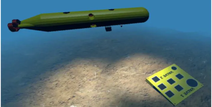
Fig. 3. Vehicle visualised in the simulated sea bottom environment above the visual target
The following model of hydrodynamic damping force and torque is used in the system dynamics [Fossen, 2002]:{
FD= −DVlVa− DVn[|Va1|Va1 |Va2|Va2 |Va3|Va3]⊤
ΓD= −DΩlΩ− DΩn[|ω1|ω1 |ω2|ω2 |ω3|ω3]⊤
(21) with damping matrices DVl, DVn, DΩl and DΩn, the
apparent velocity Va=[Va1, Va2, Va3]⊤,V−R⊤vcur, and
the current velocity vcur expressed in the inertial frame.
The physical parameters of the simulated vehicle, given in Tab. 1, closely follow that of a real AUV.
Specification Numerical value Mass m [kg] 1000 Volume [m3] 0.97 l[m] 0.15 rC[m] [1, 0, 0.5] J0[kg.m2] [ 500 −15 −25 −15 3000 −10 −25 −10 3000 ] M11 A [kg] 10 3 diag(0.07, 1.5, 1.5) M22 A [kg.m 2 ] 103 diag(1.5, 15, 15) M12 A [kg.m 2] 03×3 DV l[kg.s−1 ] diag(10, 30, 30) DV n[kg.m−1] diag(100, 300, 300) DΩl[kg.m2.s−1 ] diag(5, 15, 15) DΩn[N.m] diag(50, 150, 150)
Table 1. Specifications of the simulated AUV. • Simulation 1: This simulation is dedicated to the per-formance comparison between the proposed HBVS con-trol approach and the “standard” kinematic HBVS (i.e., Eqs. (10)) in perfect situation where all measurements
are perfect and the homography matrix H is directly
calculated according to Eq. (2), with d∗ = 3 [m] and
n∗ = [−0.0858, 0.1736, −0.9811]⊤ = −R
10◦,5◦,0◦e3. In
fact, for the two control approaches we apply the same inner-loop control (8), but the reference setpoints defined by the outer-loop control are differently specified by the two approaches. More precisely, for the inner-loop control we assume that the system’s dynamics and parameters are perfectly known in the sense that “real” physical param-eters of the vehicle and the expressions (21) of FD and
ΓD are used in the computation of the inner-loop control.
Thus, it is unnecessary to activate the integrator parts (i.e., setting kiV = kiΩ = 0). The gains and parameters
(other than those involved in the integrators (5a)-(5b)) for the inner-loop control (8) are chosen as follows:
KV = 103diag(0.93, 0.464, 2.5) KΩ= 10 4 diag(0.759, 5.623, 1.8) ∆V = diag(1500, 1500, 1500) ∆Ω= diag(375, 750, 750) (22) As for the outer-loop control corresponding to the pro-posed approach, the gains and parameters are given as:
• k1= 1.5, k2= 4, kz= 8, ∆ = 10, ∇ = 5;
• k3= 0.81, k4= 1.8, ∆ω= 10, kω= 0.1.
As for the outer-loop control corresponding to the “stan-dard” kinematic HBVS, the reference velocities are set as:{
Ωr , −λΘeΘ, VCr, −λpep
Vr , VCr− Ωr× rC
where epand eΘare given by Eq. (9) with m∗= −e3. The
gains are chosen as λp = 1.5 and λΘ = 0.9, allowing the
two control approaches to have closely similar convergence rates. The derivative terms of the reference velocities are set equal to zero, since the derivative terms ˙epand ˙eΘare
not available for the computation of the controller. Initial conditions are as follows: p(0) = [−3, −2, −4]⊤[m],
Rϕ,θ,ψ(0) = R−π 12,
π
8,π, V(0) = Ω(0) = 0 [m/s]. This
implies that pC(0) ≈ [−4.1, −2.1, −3.9]⊤[m]. The initial
yaw error is very large, i.e., eψ(0) = π, allowing one to verify the large stability domain of the proposed controller. Variations w.r.t. time of the vehicle’s position and orien-tation errors –corresponding to the standard kinematic HBVS and the proposed HBVS– are reported in Figs. 4 and 5, respectively. One observes that for both control approaches the position and orientation errors converge to zero despite large initial yaw error. However, the perfor-mance of the standard kinematic HBVS approach is rather poor. Too much oscillation occurs in position error and the vehicle even makes an unnecessary 2π-rotation about the roll axis. On the contrary, the performance of the proposed HBVS approach is quite satisfying (see Fig. 5).
• Simulation 2: This simulation is devised to test the ro-bustness of the proposed controller. First, the homography matrix H is now estimated from the observed images using OpenCV functions. Second, to test the robustness w.r.t. imperfect knowledge on the external forces and torques, in the computation of the inner-loop control (8) we simply set to zero the terms FD and ΓD, while their
expres-sion (21) is still used in the simulated dynamics. A sea current velocity vcur = [0, 1, 0]⊤[m/s] is also introduced.
Third, realistic actuation limitations are also taken into ac-count by setting physical saturations for the control thrust force and torque vectors at [±2000, ±2000, ±2000] [N ] and [±500, ±1000, ±1000] [N.m], respectively. Finally, the
fol-0 5 10 15 20 25 30 35 40 45 50 −200 −100 0 100 200 time [s] φ, Θ, ψ [d eg ] φ Θ ψ −4 −3 −2 −1 0 pC [m ] pC,1 pC,2 pC,3
Fig. 4. Standard kinematic HBVS approach: Position and orientation errors vs. time (Sim. 1).
0 5 10 15 20 25 30 35 40 45 50 −200 −150 −100 −50 0 50 time [s] φ, Θ, ψ [d eg ] φ Θ ψ −4 −3 −2 −1 0 pC [m ] pC,1 pC,2 pC,3
Fig. 5. Proposed HBVS approach: Position and orientation errors vs. time (Sim. 1).
lowing “erroneous” estimated parameters are used in the inner-loop control instead of the real values:
• ˆJ0= diag(550, 2600, 3200) [kg.m2]; • ˆM11 A = 10 3diag(0.05, 1.33, 1.33) [kg]; • ˆM22 A = 10 3diag(1.7, 13, 17) [kg.m2].
The control gains and other parameters involved in the computation of the control inputs are chosen as follows:
• kiV= 0.2, kiΩ= 0.05, kzV= kzΩ= 1, δV= 10, δΩ= 10;
• KV, KΩ, ∆V and ∆Ωare given in Eq. (22);
• k1= 0.4, k2= 1, kz= 8, ∆ = 10, ∇ = 5;
• k3= 0.64, k4= 1.6, ∆ω= 10, kω= 0.1.
The gains of the outer-loop control (i.e., k1,2,3,4) are chosen
smaller than in Sim. 1 so as to reduce the chattering effect due to measurement noises. Initial conditions of the vehicle are given by: p(0) = [0, −3, −4]⊤, R
ϕ,θ,ψ(0) = Rπ 12, π 8, 3π 4, V(0) = Ω(0) = 0. Thus, pC(0) ≈ [−0.7, −2.1, −4.4]⊤[m].
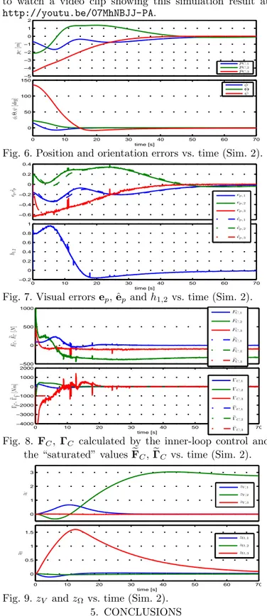
Simulation results are reported in Figs. 6–9. Fig. 7 shows that the visual errors ep and h1,2 (computed from the
estimated homography matrix) and the augmented vari-able ˆep converge to zero. One can observe the noise
ef-fects induced by imperfect homography matrix estimated from image processing. Fig. 6 shows the convergence of position and orientation errors to zero. Overshoots occur mainly due to important unknown disturbance force FD.
However, thanks to the integral action in the inner-loop control, the controller manages to compensate for this force as well as other model errors, and thus still ensures asymptotical stability. The effect of the sea current on the integral terms zV and zΩ is illustrated in Fig. 9, where
the second component of zV well converges to a
non-null value. The evolution of the control force and torque vectors w.r.t. time is shown in Fig. 8 where torque control saturation occurred in a short period of time marginally affects the overall control performance. The control forces in the directions −→eb
2 and −→eb3 asymptotically converge to
the values dictated by the compensation of the current and
buoyancy, respectively. Finally, the reader is encouraged to watch a video clip showing this simulation result at http://youtu.be/07MhNBJJ-PA. 0 10 20 30 40 50 60 70 0 50 100 150 time [s] φ, Θ, ψ [d eg ] φ Θ ψ −5 −4 −3 −2 −1 0 1 2 pC [m ] pC,1 pC,2 pC,3
Fig. 6. Position and orientation errors vs. time (Sim. 2).
0 10 20 30 40 50 60 70 −0.2 0 0.2 0.4 0.6 0.8 1 h1,2 time [s] −0.6 −0.4 −0.2 0 0.2 0.4 ep , ˆ ep ep ,1 ep ,2 ep ,3 ˆ ep ,1 ˆ ep ,2 ˆ ep ,3
Fig. 7. Visual errors ep, ˆep and h1,2vs. time (Sim. 2).
0 10 20 30 40 50 60 70 −4000 −3000 −2000 −1000 0 1000 2000 time [s] ΓC ,e ΓC [N m ] ΓC,1 ΓC,2 ΓC,3 e ΓC,1 e ΓC,2 e ΓC,3 −500 0 500 1000 FC , e F[NC ] FC,1 FC,2 FC,3 e FC,1 e FC,2 e FC,3
Fig. 8. FC, ΓC calculated by the inner-loop control and
the “saturated” values eFC, eΓC vs. time (Sim. 2).
0 10 20 30 40 50 60 70 0 0.5 1 1.5 time [s] zΩ zΩ ,1 zΩ ,2 zΩ ,3 0 1 2 3 zV zV,1 zV,2 zV,3
Fig. 9. zV and zΩvs. time (Sim. 2).
5. CONCLUSIONS
The stabilisation of fully-actuated AUVs using image-based homography matrix opens a way to several new applications of autonomous vehicles, for example the in-spection of underwater objects, too risky using traditional acoustic means. Underwater docking on flat targets can also benefit from this development. Using relatively avail-able and cheap technology of underwater vision, navigation in a structured environment can be carried out using math-ematically efficient formulation, rather than complicated
pose reconstruction from multiple sensors. A testing cam-paign with a real AUV is now envisioned so as to validate the proposed approach in the challenging sea environment.
REFERENCES
S. Benhimane and E. Malis. Homography-based 2D Visual Tracking and Servoing. Int. J. of Robotics Research, 26 (7):661–676, 2007.
S.P. Bhat and D.S. Bernstein. A topological obstruction to continuous global stabilization of rotational motion and the unwinding phenomenon. Systems & Control Letters, 39(1):63–70, 2000.
F. Chaumette and S. Hutchinson. Visual servo control, Part I: Basic approaches. IEEE Robotics and Automa-tion Magazine, 13(4):82–90, 2006.
H. de Plinval, P. Morin, P. Mouyon, and T. Hamel. Vi-sual servoing for underactuated VTOL UAVs: A linear, Homography-Based framework. Int. J. of Robust and Nonlinear Control, 2013.
T. I. Fossen. Marine Control Systems. Marine Cybernetix AS, 2002.
T. F. Gon¸calves, J. R. Azinheira, and P. Rives. Vision-based Autonomous Approach and Landing for an
Air-craft using a Direct Visual Tracking Method. In
Int. Conf. on Informatics in Control, Automation and Robotics, pages 94–101, 2009.
N. Guenard, T. Hamel, and R. Mahony. A practical visual servo control for an unmanned aerial vehicle. IEEE Trans. on Robotics, 24(2):331–340, 2008.
M.-D. Hua, T. Hamel, P. Morin, and C. Samson. A control approach for thrust-propelled underactuated vehicles and its application to VTOL drones. IEEE Trans. on Automatic Control, 54(8):1837–1853, 2009.
H. K. Khalil. Nonlinear systems. Macmillan Publishing Company, 1992.
S. Krupinski, G. Allibert, M.-D. Hua, and T. Hamel. Pipeline tracking for fully-actuated autonomous under-water vehicle using visual servo control. In American Control Conf., pages 6196–6202, 2012.
H. Lamb. Hydrodynamics. Cambridge Univ. Press, 1932. N. E. Leonard. Stability of a bottom-heavy underwater
vehicle. Automatica, 33(3):331–246, 1997.
J.-E Lots, D. M. Lane, E. Trucco, and F. Chaumette. A 2-D visual servoing for underwater vehicle station keeping. In IEEE Int. Conf. on Robotics and Automation, pages 2767–2772, 2001.
N. Metni, T. Hamel, and F. Derkx. Visual Tracking
Control of Aerial Robotic Systems with Adaptive Depth Estimation. In IEEE Conf. on Decision and Control, pages 6078–6084, 2005.
P. Rives and J.-J. Borrelly. Underwater Pipe Inspection Task using Visual Servoing Techniques. In IEEE Int. Conf. on Intelligent Robots and Syst., pages 63–68, 1997.
Appendix A. PROOF OF PROPOSITION 3 The proof is based on the analysis of the Lyapunov func-tion candidate Linner , 12W¯⊤MTW¯ + mgl(1−e⊤3R⊤e3),
with ¯W, [ ¯V⊤ Ω¯⊤]⊤. After some tedious computation, it
can be verified that the derivative of Lvalong any solution
to the closed-loop system satisfies ˙
Linner = − ¯V⊤satc∆V(KVV) − ¯¯ Ω
⊤satc
∆Ω(KΩΩ)¯
−mglkω|e3× R⊤e3|2. (A.1)
By application of Barbalat’s lemma, one deduces the convergence of ˙Linner and, thus, of ¯V, ¯Ωand 1 − e⊤3R⊤e3
to zero. The latter implies that Re3 converges to ±e3.
Let us now prove the local exponential stability (L.E.S.) of the equilibrium ( ¯V, ¯Ω, Re3) = (0, 0, e3). By denoting Θ the
angle between Re3 and e3, i.e., cos(Θ) = e⊤3Re3, around
a small neighborhood of the equilibrium ( ¯V, ¯Ω, Re3) =
(0, 0, e3) the Lyapunov function Linner can be locally
approximated by Linner≈ 0.5 ¯W⊤MTW¯ + 0.5mglΘ2and
its derivative (A.1) is approximatively given by ˙Linner ≈
− ¯V⊤K
VV− ¯¯ Ω⊤KΩΩ−mglk¯ ωΘ2. As a consequence, there
exists a positive number α such that locally ˙Linner ≤
−αLinner. This ensures the L.E.S. of Linner about zero
and, thus, the L.E.S. of the equilibrium ( ¯V, ¯Ω, Re3) =
(0, 0, e3). Finally, the exponential convergence of ¯V and
¯
Ωto zero naturally leads to same property of eVand eΩas a consequence of the technical lemma 7 (Append. D). The proof of instability of the equilibrium ( ¯V, ¯Ω, Re3) =
(0, 0, −e3) is based on the Chetaev’s theorem. Define
y = [y1 y2 y3]⊤ , e3+ Re3 and consider the following
continuously differentiable function: S(y) , y3 = 1 +
e⊤
3Re3 ≥ 0, which is null at the origin, i.e., S(0) = 0.
For some positive number r > 0, define a set Ur , {y |
S(y) > 0, |y| < r}, and note that Ur is non-null for all
r > 0. By neglecting all high-order terms, the derivative of S can be approximatively given by
˙ S ≈ e⊤
3RΩr×e3= kω|e3×Re3|2= kω|e3×y|2= kω(y21+y 2 2).
The positivity of y3is equivalent to the positivity of y12+y 2 2.
Thus, for all y ∈ Ur one ensures that ˙S > 0. Since all
the conditions of Chetaev’s theorem are satisfied [Khalil, 1992], the origin y = 0 of the linearized system is unstable.
Appendix B. PROOF OF PROPOSITION 5 Using Eqs. (12) and (17), one deduces
˙ep= −Ω×ep− a∗Ωrׯzp− a∗k1ˆep+ γ( eV, eΩ), (B.1)
with γ( eV, eΩ) , a∗( eV+ eΩ
×rc) + eΩ×m∗, ¯zp , zp− z∗p.
From here, the proof proceeds by three steps:
Step 1:We will show that zpis bounded by some constant.
Consider the positive function S1, 0.5|zp|2. Its derivative
satisfies (using (16)) ˙S1 ≤ −kz|zp|2+ |zp|( ¯Ωr∇ + kz∆),
with ¯Ωr , sup(|Ωr|). From here, it is straightforward to
deduce that ∀t ≥ 0
|zp(t)| ≤ ( ¯Ωr∇)/kz+∆ = ∆(1+α ¯Ωr), with α, ∇/(kz∆).
Step 2:We will show next that there exists a time instant
T such that ∀τ ≥ T one has |ep(τ )| ≤ ∇ and, thus,
sat∇(e
p(τ )) = ep(τ ). Denote X , [x y]⊤ ∈ R6, with
x, Rˆep, y, Rep. One verifies from (16) and (B.1) that
˙ X= [ −k2I3 k2I3 −a∗k1I3 0 ] | {z } =:A∈R6×6 X+ [ 0 R(−a∗Ω rׯzp+γ( eV, eΩ)) ] | {z } =:B∈R6 (B.2) The condition (18) ensures that A has two triple distinct real negative eigenvalues λ1,2 (λ1 < λ2 < 0) given by
λ1,2 = 0.5(−k2∓
√ k2
2− 4a∗k1k2). This implies that A
is diagonalisable and can be decomposed in the Jordan
normal form A = PΛP−1, with Λ = diag(λ
1I3, λ2I3) and P= λ1I3 η1 λ2I3 η2 −a∗ 1k1I3 η1 −a∗ 1k1I3 η2 , P−1= 1 λ2−λ1 −η1I3 −λ2η1I3 a∗ 1k1 η2I3 λ1η2I3 a∗ 1k1 η1, √ λ2 1+ (a∗1k1)2, η2, √ λ2 2+ (a∗1k1)2.
(λ2−λ1) 2 |P−1X|2= η21 x + λ 2 (a∗k 1) y 2 + η22 x + λ 1y a∗k 1 2 = √ η2 1+η 2 2 ( x+λ1y a∗k1 ) +η 2 1(λ2−λ1)y a∗k 1 √ η2 1+η 2 2 2 +η 2 1η 2 2(λ2−λ1)2|y|2 (a∗k1)2(η2 1+η 2 2) , which allows one to deduce
|P−1X| ≥ η1η2 a∗k1√η2 1+η 2 2 |y| = η1η2 a∗k1√η2 1+η 2 2 |ep|. (B.3)
On the other hand, as a result of Proposition 3, eΩ and e
V are uniformly continuous and bounded, and converge
asymptotically to zero. Consequently, γ( eV, eΩ) also con-verges to zero. Thus, for some positive number ε (to be specified hereafter) there exists a time instant T1such that
∀t ≥ T1one has |γ( eV, eΩ)| ≤ ε. Then, ∀t ≥ T1one verifies
|P−1B| = √ λ2 1η 2 2+ λ 2 2η 2 1 a∗k 1(λ2−λ1) −a∗Ωrׯzp+γ( eV, eΩ) ≤ √ λ2 1η 2 2+ λ 2 2η 2 1 a∗k 1(λ2−λ1) (( a∗∆(1 + α ¯Ωr)+1) ¯Ωr+ε ) . (B.4)
Using Eq. (B.2), the derivative of S2 , 0.5|P−1X|2
satisfies ˙ S2 = (P−1X)⊤Λ(P−1X) + (P−1X)⊤(P−1B) ≤ λ2|P−1X| 2 + |P−1X| |P−1B|. (B.5)
Since zp, Ωr, eΩ and eV are bounded, B and P−1B are
also bounded. From Eq. (B.5) and the definition of S2,
one ensures that P−1Xand X are bounded w.r.t. initial
conditions. Consequently, epand ˆepremain bounded w.r.t.
initial conditions. Then, it is straightforward to verify that ˙ep, ˙ˆep and ˙zp are bounded w.r.t. initial conditions, which
implies the uniform continuity of ep, ˆep and zp.
Since X remains bounded w.r.t. initial conditions on the time-interval [0, T1] (as proved previously), from Eq. (B.5)
and the definition of S2 there exists another time-instant
T > T1such that ∀τ ≥ T one has
|P−1X(τ )| ≤ (−λ 2)−1sup
t≥T
(|P−1B(t)|). (B.6)
In view of Eqs. (B.3), (B.4) and (B.6) one deduces that |ep(τ )| ≤ ¯∇ + ε √ (η2 1+η 2 2)(λ 2 1η 2 2+λ 2 2η 2 1) λ2(λ1−λ2)η1η2 , ∀τ ≥ T, (B.7) with ¯ ∇, √ (η2 1+η 2 2)(λ 2 1η 2 2+λ 2 2η 2 1) λ2(λ1−λ2)η1η2 ( a∗∆(1 + α ¯Ω r)+1) ¯Ωr> 0.
Therefore, if ∇ is chosen larger than ¯∇ (i.e., ∇ > ¯∇) and if ε is chosen such that
0 < ε < (∇ − ¯√ ∇)λ2(λ1−λ2)η1η2 (η2 1+η 2 2)(λ 2 1η 2 2+λ 2 2η 2 1) ,
then one deduces from inequality (B.7) that |ep(τ )| < ∇,
∀τ ≥ T , and thus sat∇(e
p(τ )) = ep(τ ).
Step 3:Consider the Lyapunov candidate function
L, 1/(2a∗)|e
p|2+ k1/(2k2)|ˆep|2+ 1/2|¯zp|2.
Using the following property [Hua et al., 2009]: |sat∆ (x + c) − c| ≤ |x|, ∀(c, x) ∈ R3 × R3 with |c| ≤ ∆, one deduces ˙ L = −k1|ˆep| 2 + ¯z⊤pΩr×(ep− sat∇(ep)) + 1/a∗e⊤pγ( eV, eΩ) −kz¯z⊤p(¯zp+ z∗p− sat ∆ (¯zp+ z∗p)) ≤ −k1|ˆep|2+ ¯z⊤pΩr×(ep− sat∇(ep)) + 1/a∗e⊤pγ( eV, eΩ). Since sat∇(e p(τ )) = ep(τ ) and |ep(τ )| ≤ ∇, ∀τ ≥ T (as
proved in Step 2), one obtains
˙
L(τ ) ≤ −k1|ˆep(τ )| 2
+ ∇/a∗|γ( eV(τ ), eΩ(τ ))| . (B.8) As proved previously, ep, ˆepand zpcannot escape in
finite-time. Thus, L(t) remains bounded on the time-interval [0, T ]. In addition, ep(τ ), ˆep(τ ), zp(τ ) and, thus, L(τ ),
∀τ ≥ T , remain bounded by some positive constants inde-pendent from all initial conditions (as proved previously). Since the equilibrium ( eV, eΩ, R⊤e
3) = (0, 0, e3) is locally
exponentially stable as a result of Proposition 3, there exist some time-instant T2> T and some positive constants α1
and α2 such that
γ( eV(τ ), eΩ(τ )) ≤ α1e−α2τ, ∀τ ≥ T2. (B.9)
From Eqs. (B.8) and (B.9), one deduces ˙
L(τ ) ≤ −k1|ˆep(τ )|2+ (α1∇)/a∗e−α2τ, ∀τ ≥ T2.
Consequently, by integration one deduces
∫ ∞ T2 |ˆep(τ )|2dτ ≤ α1∇e−α2T2 k1α2a∗ + 1 k1 (L(T2) − L(∞)).
From here, the resulting boundedness of integral term ∫∞
T2 |ˆep(τ )|
2
dτ and the uniform continuity of ˆep implies
the convergence of ˆep to zero (Barbalat’s lemma).
From Eq. (16), one verifies that ˙ˆep can be rewritten as
˙ˆep(t) = a(t) + b(t), with a(t) , k2ep the uniformly
continuous term and b(t), −Ω׈ep− k2ˆep the vanishing
term. Then, the application of the extended Barbalat’s lemma [Hua et al., 2009] ensures the convergence of ˙ˆep to
zero, which in turn implies the convergence of ep to zero.
Appendix C. PROOF OF THEOREM 6
From (20), it is straightforward that ω3r and ˙ω3r remain
bounded by k3∆ω/k4and 2k3∆ω, respectively. The
bound-edness of ω3r and ˙ω3r is a necessary condition of
Propo-sitions 3 and 5. One ensures that at the zero dynamics ˙
ψ = ω3 = ω3r and h1,2 = sin ψ ≤ 1 < ∆ω. Thus, at the
zero dynamics, the dynamics of ω3rgiven by (20) satisfies
˙ω3r= −k4ω3r− k3sin ψ. (C.1)
Consider the positive function SΘ, k3(1 − cos ψ) +12ω32r.
Using (C.1), one obtains ˙SΘ = −k4ω32r ≤ 0. The
ap-plication of LaSalle principle ensures the convergence of ˙
SΘ and, thus, of ω3r to zero. Then, Barbalat’s lemma
ensures the convergence of ˙ω3r to zero. One deduces the
convergence of sin ψ to zero. From here, one deduces the existence of two isolated equilibria of H corresponding
to two values of ψ = ψ⋆
1 , 0 and ψ = ψ⋆2 , π. The
equilibrium ψ = 0 corresponds to the desired equilibrium
H= H⋆
1, I3and the other one ψ = π corresponds to the
undesired equilibrium H = H⋆
2, diag(−1, −1, 1).
To prove the local stability results, it suffices to study the linearized system about the equilibrium. For the equilib-rium ψ = 0, the linearized system is
˙˜
ψ = ω3, ˙ω3= −k4ω3− k3ψ˜
with ˜ψ = ψ. Since its characteristic polynomial p2
+ k4p +
k3is Hurwitz, the equilibrium ψ = ψ1⋆= 0 is exponentially
stable. On the other hand, the linearized systems for the equilibrium ψ = π is given by:
˙˜
ψ = ω3, ˙ω3= −k4ω3+ k3ψ˜
with ˜ψ = ψ − π. Using Hurwitz criteria, one easily verifies that the origin of this linearized system is unstable.
Appendix D. TECHNICAL LEMMA
Lemma 7. (Omitted proof) If x(t) + k∫tt0x(τ )dτ , with
x ∈ Rn and k > 0, converges exponentially to some