Water restrictions under climate change: a Rhône-Mediterranean perspective combining bottom-up and top-down approaches

HAL Id: hal-02609677

https://hal.inrae.fr/hal-02609677

Submitted on 16 May 2020

HAL is a multi-disciplinary open access

archive for the deposit and dissemination of

sci-entific research documents, whether they are

pub-lished or not. The documents may come from

teaching and research institutions in France or

abroad, or from public or private research centers.

L’archive ouverte pluridisciplinaire HAL, est

destinée au dépôt et à la diffusion de documents

scientifiques de niveau recherche, publiés ou non,

émanant des établissements d’enseignement et de

recherche français ou étrangers, des laboratoires

publics ou privés.

Rhône-Mediterranean perspective combining bottom-up

and top-down approaches

Eric Sauquet, B. Richard, Alexandre Devers, C. Prudhomme

To cite this version:

Eric Sauquet, B. Richard, Alexandre Devers, C. Prudhomme. Water restrictions under climate change:

a Rhône-Mediterranean perspective combining bottom-up and top-down approaches. Hydrology and

Earth System Sciences, European Geosciences Union, 2019, 23, pp.3683-3710.

�10.5194/hess-23-3683-2019�. �hal-02609677�

https://doi.org/10.5194/hess-23-3683-2019 © Author(s) 2019. This work is distributed under the Creative Commons Attribution 4.0 License.

Water restrictions under climate change: a Rhône–Mediterranean

perspective combining bottom-up and top-down approaches

Eric Sauquet1, Bastien Richard1,2, Alexandre Devers1, and Christel Prudhomme3,4,5

1_{UR RiverLy, Irstea, 5 Rue de la Doua CS20244, 69625 Villeurbanne CEDEX, France}

2_{UMR G-EAU, Water Resource Management, Actors and Uses Joint Research Unit, Campus Agropolis, Irstea,}

361 Rue Jean-François Breton, BP 5095, 34196 Montpellier CEDEX 5, France

3_{European Centre for Medium-range Weather Forecast, Shinfield Road, Reading, RG2 9AX, UK} 4_{Department of Geography, Loughborough University, Loughborough, LE11 3TU, UK}

5_{NERC Centre for Ecology & Hydrology, Maclean Building, Benson Lane,}

Crowmarsh Gifford, Wallingford, Oxon, OX10 8BB, UK Correspondence: Eric Sauquet (eric.sauquet@irstea.fr)

Received: 28 August 2018 – Discussion started: 11 September 2018

Revised: 15 July 2019 – Accepted: 24 July 2019 – Published: 13 September 2019

Abstract. Drought management plans (DMPs) require an overview of future climate conditions for ensuring long-term relevance of existing decision-making processes. To that end, impact studies are expected to best reproduce decision-making needs linked with catchment intrinsic sensitivity to climate change. The objective of this study is to apply a risk-based approach through sensitivity, exposure and perfor-mance assessments to identify where and when, due to cli-mate change, access to surface water constrained by legally binding water restrictions (WRs) may question agricultural activities. After inspection of legally binding WRs from the DMPs in the Rhône–Mediterranean (RM) district, a frame-work to derive WR durations was developed based on harmo-nized low-flow indicators. Whilst the framework could not perfectly reproduce all WR ordered by state services, as devi-ations from sociopolitical factors could not be included, it en-abled the identification of most WRs under the current base-line and the quantification of the sensitivity of WR duration to a wide range of perturbed climates for 106 catchments. Four classes of responses were found across the RM district. The information provided by the national system of compen-sation to farmers during the 2011 drought was used to de-fine a critical threshold of acceptable WR that is related to the current activities over the RM district. The study finally concluded that catchments in mountainous areas, highly sen-sitive to temperature changes, are also the most predisposed to future restrictions under projected climate changes

consid-ering current DMPs, whilst catchments around the Mediter-ranean Sea were found to be mainly sensitive to precipita-tion changes and irrigaprecipita-tion use was less vulnerable to pro-jected climatic changes. The tools developed enable a rapid assessment of the effectiveness of current DMPs under cli-mate change and can be used to prioritize review of the plans for those most vulnerable basins.

1 Introduction

The Mediterranean region is known as one of the “hotspots” of global change (Giorgi, 2006; Paeth et al., 2017) where en-vironmental and socio-economic impacts of climate change and human activities are likely to be very pronounced. The intensity of the changes is still uncertain; however, climate models agree on a significant future increase in frequency and intensity of meteorological, agricultural and hydrolog-ical droughts in southern Europe (Jiménez Cisneros et al., 2014; Touma et al., 2015), with climate change likely to ex-acerbate the variability in climate with regional feedbacks affecting Mediterranean-climate catchments (Kondolf et al., 2013). Facing more severe low flows and significant losses of snowpack, southeastern France will be subject to substantial alterations of water availability; Chauveau et al. (2013) have shown a potential increase in low-flow severity by the 2050s with a decrease in low-flow statistics to 50 % for the Rhône

river near its outlet. Andrew and Sauquet (2017) have re-ported that global change will most likely result in a decrease in water resources and an increase both in pressure on water resources and in occurrence of periods of water limitation within the Durance river basin, one of the major water tow-ers of southeastern France. In addition, Sauquet et al. (2016) have suggested the need to open the debate on a new fu-ture balance between the competing water uses. More re-cently, based on climate projections obtained from the Cou-pled Model Intercomparison Project Phase 5 (Taylor et al., 2012), Dayon et al. (2018) have identified a significant in-crease in hydrological drought severity with a meridional gradient (up to −55 % in southern France for both the annual minimum monthly flow with a return period of 5 years and the mean summer river flow), while a more uniform increase in agricultural drought severity is projected over France for the end of the 21st century.

The challenges associated with possible impact of climate change on droughts have received increasing attention by researchers, stakeholders and policymakers in the previous decades. To date climate change impact studies are usually dedicated to water resources (e.g. Vidal et al., 2016; Collet et al., 2018; Hellwig and Stahl, 2018; Samaniego et al., 2018) or water needs for the competing users (e.g. Bisselink et al., 2018). However, examining the suitability of regulatory in-struments, such as drought management plans (DMPs), is also essential in establishing successful adaptation strategies. These plans state which type of water restrictions (WRs) should be imposed to non-priority uses during severe low-flow events; under climate change, those water restrictions and stakeholders’ access to water resources might need to be revised, as drought patterns and severity might change. In most climate change impact studies, analyses on the regula-tory measures are often limited to maintaining environmental flows – especially when assessing future hydropower poten-tial. To date, no climate change impact on water regulatory measures has yet been assessed at the regional scale, high-lighting a gap in developing robust adaptation plans. This study aims to address this gap by suggesting a framework, applying it to southeastern France and publishing the associ-ated results.

The paper develops a framework to simulate legally bind-ing WRs under climate change in the Rhône–Mediterranean (RM) district (southeastern France) and to assess the like-lihood of future restrictions depending on their sensitivity, performance and exposure to climate deviations. The approach is adapted from the risk-based approaches such as those developed in parallel by Brown et al. (2011) – called the “decision tree framework” – and Prudhomme et al. (2010) – called the “scenario-neutral approach” – and aims to establish a ranking of areas vulnerable to climate change in terms of water access for agricultural uses. This research is a scientific contribution to the ongoing initiative of the decade 2013–2022 entitled “Panta Rhei – Everything Flows” initiated by the International Association of

Hy-drological Sciences and more specifically to the “Drought in the Anthropocene” working group (https://iahs.info/ Commissions--W-Groups/Working-Groups/Panta-Rhei/ Working-Groups/Drought-in-the-Anthropocene.do, last access: 1 August 2019, Van Loon et al., 2016). Legally binding water restrictions and their associated decision-making processes are important for the blue water footprint assessment at the catchment scale.

The paper is organized in four parts. Section 2 introduces the area of interest and the source of data. Section 3 is a syn-thesis of the mandatory processes for managing drought con-ditions implemented within the Rhône–Mediterranean dis-trict and the related water-resdis-triction orders adopted over the period 2005–2016. Section 4 describes the general mod-elling framework developed to simulate WR decisions. The approach is implemented at both local and regional scales, and results are discussed in Sect. 5 before drawing general conclusions in Sect. 6.

2 Study area and materials 2.1 Study area

The Rhône–Mediterranean district covers all the Mediter-ranean coastal rivers and the French part of the Rhône river basin, from the outlet of Lake Geneva to its mouth (Fig. 1). Climate is rather varied, with a temperate influence in the north, a continental influence in the mountainous areas, and a Mediterranean climate with dry and hot summers dominating in the south and along the coast. In the mountainous part (in both the Alps and the Pyrenees) the snowmelt-fed regimes are observed in contrast to the northern part under oceanic climate influences, where seasonal variations in evaporation and precipitation drive the monthly runoff pattern (Sauquet et al., 2008).

Water is globally abundant but uneven between the moun-tainous areas and the northern and southern parts of the RM district, and water resources are under high pressure due to water abstractions. For the period 2008–2013, an-nual total water withdrawal was around 6 × 109m3 (exclud-ing any water abstraction for energy such as cool(exclud-ing nu-clear plants and hydropower) with more used for irriga-tion (3.4 × 109m3, including 2 × 109m3 for channel con-veyance). Use for public and industrial supply is 1.6 × 109 and 1 × 109m3, respectively. Because of an intense competi-tion for water between different users – agricultural, munic-ipal and industrial – and the environment, some areas within the RM district can be vulnerable during low-flow periods. Around 40 % of the RM district suffers from water stress and scarcity (http://www.rhone-mediterranee.eaufrance.fr/ gestion/gestion-quanti/problematique.php, last access: 1 Au-gust 2019) and has been identified by the French RM Wa-ter Agency as areas with persistent imbalance between waWa-ter supply and water demand.

Figure 1. The Rhône–Mediterranean water district, the total num-ber of WR decisions stated by department over the period 2005– 2016 and the gauged catchments (◦) where WR decisions are simu-lated (• denotes the subset of the 15 catchments used for evaluation purposes, and the figures are the related ranks presented in Table 1).

2.2 Drought management plan

DMPs define specific actions to be undertaken to enhance preparedness and increase resilience to drought. In France DMPs include regulatory frameworks to be applied in case of drought, called arrêtés cadres sécheresse. The past and oper-ating DMPs and the water-restriction orders were inspected in the 28 departments of the RM district. They were obtained from the following:

– the database of the DREAL Auvergne-Rhône-Alpes (“Direction Régionale de l’Eau, de l’Alimentation et du Logement” in French), including water-restriction lev-els (WRLs) and duration at the catchment scale avail-able over the period 2005–2016 within the RM district, – the online national database PROPLUVIA (http:// propluvia.developpement-durable.gouv.fr, last access: 1 August 2019), with WRLs and dates of adoption at the catchment scale for the whole of France available from 2012.

The most recent consulted documents date from Jan-uary 2017.

2.3 Hydrological data

The hydrological observation dataset is a subset of the 632 French near-natural catchments identified by Caillouet et al. (2017). Daily flow data from 1958 to 2013 were extracted from the French HYDRO database (http://hydro.eaufrance. fr/, last access: 1 August 2019). Time series with more than

30 % missing values or more than 30 % null values were dis-regarded. Finally, the total dataset consists of 106 gauged catchments located in the RM district, with minor human in-fluence and with high-quality data. The selected catchments are benchmark catchments where near-natural drought events are observed and current water availability is monitored. Wa-ter can be abstracted from other nearby streams.

A selection of 15 evaluation catchments (Table 1) were used to calibrate and to evaluate the WRL (WR level) mod-elling framework (Sect. 4), selected because (i) they have complete records of stated water restriction, including dates and levels of restrictions – which was not the case in other catchments – and (ii) they are located in areas where water-restriction decisions are frequent. To facilitate interpretation, the 15 catchments were ordered along the north–south gra-dient. The Ouche and Argens river basins (no. 1 and 15 in Table 1) are the northernmost and the southernmost gauged basins, respectively. The 15 catchments encompass a large variety of river flow regimes according to the classification suggested by Sauquet et al. (2008; see Appendix A) that can be observed in the RM district (e.g. the Ouche – 1 in Table 1, pluvial regime; Roizonne – 3, transition regime; and Argens – 15, snowmelt-fed regime – river basins).

2.4 Climate data

Baseline climate data were obtained from the French near-surface Safran meteorological reanalysis (Quintana-Seguí et al., 2008; Vidal et al., 2010) onto an 8 km resolution grid from 1 August 1958 to 2013. Exposure data were based on the regional projections for France (Table 2) available from the DRIAS French portal (http://www.drias-climat.fr/, last access: 1 August 2019, Lémond et al., 2011). Catchment-scale data were computed as a weighted mean for tempera-ture and the sum for precipitation based on the river network described by Sauquet (2006).

3 Operating drought management plans in the Rhône–Mediterranean district

The “French Water Act” amended on 24 September 1992 (decree no. 92/1041) defines the operating procedures for the implementation of a DMP. Following the 2003 Euro-pean heat wave, drought management plans including wa-ter restrictions have been gradually implemented in France (MEDDE, 2004). Water restrictions fall within the respon-sibility of the prefecture (one per administrative unit or de-partment), as mentioned in article L211-3 II-1 of the French environmental code. Their role in drought management is to ensure that regulatory approvals for water abstraction con-tinuously meet the balance between water resource avail-ability and water uses including needs for aquatic ecosys-tems. De facto, legally binding water restrictions have to ful-fil three principles: (i) being gradually implemented at the

Table 1. Main characteristics of the 15 catchments used for validation of water-restriction simulations. Station number refers to the catchment number in the HYDRO database, and regime class refers to the classification suggested by Sauquet et al. (2008) with a gradient from Class 1 – pluvial-fed regime –F moderately contrasting with Class 12 – snowmelt-fed regime.

No. River Department Station Elevation Area Regime NSELOG KGESQRT

basin (department number) number (m a.s.l.) (km2) class

1 Ouche Côte d’Or (21) U1324010 243 651 6 0.84 0.94 2 Bourbre Isère (38) V1774010 202 703 1 0.85 0.92 3 Roizonne Isère (38) W2335210 936 71.6 11 0.71 0.84 4 Bonne Isère (38) W2314010 770 143 12 0.80 0.91 5 Buëch Hautes-Alpes (05) X1034020 662 723 9 0.84 0.93 6 Drôme Drôme (26) V4214010 530 194 3 0.81 0.89 7 V4264010 263 1150 9 0.85 0.88 8 Roubion Drôme (26) V4414010 264 186 9 0.83 0.93 9 Lot Lozère (48) O7041510 663 465 3 0.88 0.94 10

Tarn Lozère (48) O3011010 905 67 8 0.73 0.90

11 O3031010 565 189 9 0.81 0.91

12 Hérault Hérault (34) Y2102010 126 912 8 0.83 0.88 13 Asse Alpes-de-Haute-Provence (04) X1424010 605 375 9 0.80 0.86 14 Caramy Var (83) Y5105010 172 215 2 0.85 0.94 15 Argens Var (83) Y5032010 175 485 2 0.80 0.92

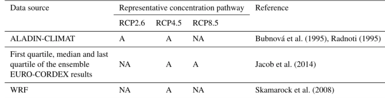
Table 2. Regional climate projections available in the DRIAS portal (A: available; NA: not available). Data source Representative concentration pathway Reference

RCP2.6 RCP4.5 RCP8.5

ALADIN-CLIMAT A A NA Bubnová et al. (1995), Radnoti (1995) First quartile, median and last

NA A A Jacob et al. (2014) quartile of the ensemble

EURO-CORDEX results

WRF NA A NA Skamarock et al. (2008)

catchment scale with regards to low-flow severity observed at various reference locations, (ii) ensuring user equity and upstream–downstream solidarity, and (iii) being time-limited to fix cyclical deficits rather than structural deficits. The pre-fecture is in charge of establishing and monitoring the DMP operating in the related department.

Past and current drought management plans were analysed to identify the past and current modalities of application, the frequency of water-restriction orders, and the areas affected by water restrictions. Gathering and studying the regulatory documents was tedious in particular because of their lack of a clear definition of the hydrological variables used in the decision-making process.

This analysis shows that the implementation of the DMPs has evolved for many departments since 2003, e.g. with changes in the terminology and a national-scale effort to stan-dardize WRLs. Now severity in low flows is classified into four levels, which are related to incentive or legally binding water restrictions. These measures affect recreational uses; vehicle washing; lawn watering; and domestic, irrigation and industrial uses (Table 3). Level 0 (called “vigilance”) refers to incentive measures, such as an awareness campaign to pro-mote low water consumption from public bodies and the gen-eral public. Levels 1 to 3 are incrementally legally binding restriction levels; level 1 (called “alert”) and 2 (called “re-inforced alert”) enforce reductions in water abstraction for agriculture uses or several days a week of suspension. Level 3

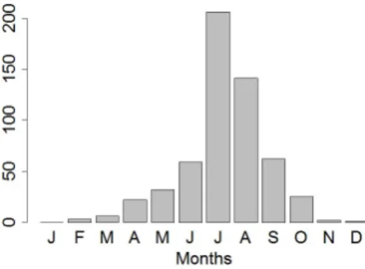
Figure 2. Total number of stated WR decisions over the RM district per month over the period 2005–2016.

(called “crisis”) involves a total suspension of water abstrac-tion for non-priority uses, including abstracabstrac-tion for agricul-tural uses and home gardening, and authorizes only water abstraction for drinking water and sanitation services. Due to change in the naming of WRLs since their creation, one task was dedicated to restate the WR decisions (hereafter “OBS”) since 2005 with respect to the current classification into four WRLs.

For all catchments, a WR decision chronology was de-rived, showing a large spatial variability in WR (Fig. 1); note that the 15 evaluation catchments (Table 1) are located in the most affected areas. Between 2005 and 2012, WR decisions were mainly adopted between April and October (98 % of the WR decisions; Fig. 2), with 62 % in July or August, peaking in July.

Decisions for adopting, revoking or upgrading a WR mea-sure are taken after consultation of “drought committees” bringing the main local stakeholders together, the meeting frequency of which is irregular and depends on hydrolog-ical drought development. The adopted restriction level is mainly based on the existing hydrological conditions at the time, i.e. based on low-flow monitoring indicators measured at a set of reference gauging stations and their departure from a set of regulatory thresholds. This varies greatly across the RM district (Fig. 3). The low-flow monitoring indicators usu-ally considered are as follows:

– the daily discharge Qdaily,

– the maximum discharge QCd for a window with length

ddays, QCd(t ) =max(Qdaily(t

0_{), t}0_{∈ [t −d +1, t ]), and}

– the mean discharge VCd for a window with length

d days, VCd(t ) = 1 d t R t −d+1 Qdaily(t0)dt0.

Both QCd and VCd are computed over the whole discharge

time series on moving time windows with duration d, asso-ciated with the WR decision varying between 2 and 10 d de-pending on DMPs. VC3 (40 % of DMPs) and QC7 (17 % of

DMPs) are the most commonly used, but other single indi-cators include Qdaily (17 %), QC5 (14 %), QC10 (8 %), QC2

(3 %) and VC10(3 %), with mixed indicators also being used

(e.g. 14 % of VC3and Qdailytogether).

The threshold associated with WR also varies within the district, generally associated with statistics derived from low-flow frequency analysis but also fixed to locally defined eco-logical requirements. In the context of DMPs, series of min-imum QCd or VCd values are calculated by the block

mini-mum approach and thereafter fitted to a statistical distribu-tion. The block is not the year but the month, or it is given by the division of the year into thirty-seven 10 d time win-dows. The regulatory thresholds are given by quantiles with four different recurrence intervals associated to the four re-striction levels. Generally, return periods T of 2, 5, 10 and 20 years are associated with the vigilance, alert, reinforced alert and crisis restriction levels, respectively. For example, let us consider thresholds based on the annual monthly min-ima of VCd. The block minimum approach is carried out on

the N years of records for each month i, i = 1 . . . , 12, leading to 12 datasets, {min{VCd(t ), month(t ) = i, year(t ) = j }, j =

1, . . . , N }. The 12 fitted distribution allows the calculation of 48 values of thresholds (month-V CNd; 12 months × 4

lev-els) with four T -year recurrence intervals.

The meteorological situation is also examined in terms of precipitation deficit and likelihood of significant rain-fall event considering available short- to medium-range weather forecasts. There are heterogeneities in the drought-monitoring variables, the time period on which deficit is cal-culated and the permissible deviation from long-term average values.

Where appropriate, other supporting local observations such as groundwater levels, reservoir water levels, field sur-veys provided by the ONDE network (Beaufort et al., 2018) or feedbacks from stakeholders can be used to inform final decisions.

Since their creation, DMPs have been frequently updated regarding the definition of the regulatory thresholds and the monitoring variables, the water uses affected by legally bind-ing restrictions, the selection of the monitorbind-ing sites, etc. It was especially done following the publication of the report of the French ministry of Ecology in May 2011, and up-dates often occur after a year with a severe drought to include feedbacks and lessons for the future. Decision-making pro-cesses are definitely heterogeneous in both time and space, which does not make the WR modelling easy. In addition, of-ficial reports stated that the DMPs were not all available for this study. Facing this complexity, simplifying assumptions will be considered in the modelling framework presented in Sect. 4.3.4 (Risk-based framework and the related tools).

Table 3. Uses affected by water restriction according to the drought severity.

Level Name Water restriction

Recreational Vehicle Lawn Swimming-pool Urban Irrigation Industry Drinking washing watering filling washing water and sanitation

0 Vigilance × × × × ×

1 Alert × × × × × × ×

2 Reinforced alert × × × × × × ×

3 Crisis × × × × × × × ×

Figure 3. Low-flow monitoring variables used in the current drought management plans. Qdailydenotes daily streamflow, QCd denotes the

d-day maximum discharge, V_Cd refers to the d-day mean discharge, and “Mixed” refers to combinations of the aforementioned variables. Department codes are given in brackets.

4 Risk-based framework and the related tools 4.1 The scenario-neutral concept

Traditionally, hydrological impact studies are often based on “top-down” (scenario-driven) approaches and easy to inter-pret, but with associated conclusions becoming outdated as new climate projections are produced. In addition scenario-based studies may fail to match decision-making needs, since the implication in terms of water management is usu-ally ignored (Mastrandrea et al., 2010). As a substitute to the scenario-driven approach, the scenario-neutral approach (Brekke et al., 2009; Prudhomme et al., 2010, 2013a, b, 2015; Brown et al., 2012; Brown and Wilby, 2012; Culley et al.,

2016; Danner et al., 2017) has been developed to better ad-dress risk-based decision issues. The suggested framework shifts the focus to the current vulnerability of the system af-fected by changes and to critical thresholds above which the system starts to fail to identify possible maladaptation strate-gies (Broderick et al., 2019). Applied to water management issues, the scenario-neutral studies (Weiß, 2011; Wetterhall et al., 2011; Brown et al., 2011; Whateley et al., 2014) aim at improving the knowledge of the system’s vulnerability to changes and at bridging the gap between scientists and stake-holders facing needs in relevant adaptation strategy. Prud-homme et al. (2010) have suggested combining of the sensi-tivity framework with top-down projections through climate

response surfaces. This approach has been applied to low flows in the UK (Prudhomme et al., 2015), and its interests have been discussed as a support tool for drought manage-ment decisions.

The risk-based framework adopted contains three indepen-dent components (Fig. 4):

i. Sensitivity analysis (Fronzek et al., 2010) is based on simulations under a large spectrum of perturbed cli-mates to (a) quantify how policy-relevant variables respond to changes in different climate factors and (b) identify the climate factors that the system is the most sensitive to. Addressing (a) and (b) may help mod-ellers in checking the relevance of their model (e.g. un-expected sensitivity to a climate factor regarding the known processes influencing the rainfall–runoff trans-formation). From an operational viewpoint, it may en-courage stakeholders to monitor, with priority, the vari-ables that affect the system of interest (reinforcement of the observation network, literature monitoring, etc.). ii. Sustainability or performance assessment aims to

iden-tify under which climate (or other) conditions (e.g. no-rain period in spring, heat wave in summer, etc.) the sys-tem fails. A key challenge in the bottom-up framework is to define performance metrics and associated critical thresholds relevant to the system of interest. In the case of our study, these thresholds will make it possible to distinguish the duration of water restrictions which is unacceptable for users.

iii. Exposure is defined by state-of-the-art regional climate trajectories superimposed to the climate response sur-face. The exposure measures the probability of changes occurring for different lead times based on available re-gional projections.

All the components of the framework together contribute to the vulnerability of the system (including its management) to systematic climatic deviations.

The sensitivity analysis was conducted by applying a water-restriction modelling framework. Climate conditions were generated by applying incremental changes to historical data (precipitation and temperature) and introduced as inputs in the developed models to derive occurrence and severity of water restriction under modified climates. The tool cho-sen here to display the interactions between water restric-tion and the parameters that reflect the climate changes is a two-dimensional response surface, with axes represented by the main climate drivers. This representation is commonly used in scenario-neutral approach. For example, in both Cul-ley et al. (2016) and Brown et al. (2012), the two axes were defined by the changes in annual precipitation and temper-ature. When changes affect numerous attributes of the cli-mate inputs, additional analyses (e.g. elasticity concept com-bined with regression analysis – Prudhomme et al., 2015;

the Spearman rank correlation and Sobol sensitivity analy-ses – Guo et al., 2017) may be required to point out the key variables with the largest influence on water restriction that form thereafter the most appropriate axes for the response surfaces.

Performance assessment is a challenging task for hydrol-ogists, since it requires information on the impact of ex-treme hydrometeorological past events on stakeholders’ ac-tivities. Simonovic (2010) used observed past events selected with local authorities on a case study in southwestern On-tario (Canada), chosen for their past impact (flood peak as-sociated with a top-up of the embankments of the main ur-ban centre; level 2 drought conditions of the low water re-sponse plan). Schlef et al. (2018) set the threshold to the worst modelled event under current conditions. Whateley et al. (2014) assessed the robustness of a water supply system, and the threshold is fixed to the cumulative cost penalties due to water shortage evaluated under the current conditions. Brown et al. (2012) and Ghile et al. (2014) suggested select-ing thresholds accordselect-ing to expert judgment of unsatisfactory performance of the system by stakeholders, whilst Ray and Brown (2015) use results from cost–benefit analyses. The spatial coverage of a large area, such as the RM district, and the heterogeneity in water use (domestic needs, hydropower, recreation, irrigation, etc.) make it challenging for a system-atic, consistent and comparable stakeholder consultation to be conducted and for a relevant critical threshold Tc to be

fixed for all the users. Facing this complexity, only the ir-rigation water use will been examined here, since it is the sector which consumes most water at the regional scale, with a critical threshold defined for this single water use.

Exposure to changes here is measured using regional pro-jections, visualized graphically by positioning the regional projections in the coordinate system of the climate response surfaces and identifying the associated likelihood of failure relative to Tc. Note that, to update the risk assessment, only

the exposure component has to be examined (including the latest climate projections available onto the response sur-faces).

4.2 The rainfall–runoff modelling

The conceptual lumped rainfall–runoff model GR6J was adopted for simulating daily discharge at 106 selected catch-ments of the RM district. The GR6J model is a modified ver-sion of GR4J originally developed by Perrin et al. (2003), which is well suited to simulate low-flow conditions (Push-palatha et al., 2011). The four-parameter version of the model GR4J has been progressively modified. Le Moine (2008) has suggested a new groundwater exchange function and a new routing store representing long-term memory in the GR5J model. Pushpalatha et al. (2011) finally introduced in the GR6J model an exponential store parallel to the existing store of the GR5J model. Considering additional routing stores is consistent regarding the natural complexity of hydrological

Figure 4. Schematic framework of the developed approach to assess the vulnerability of the DMPs under climate change.

processes, and in particular, the dynamics of flow compo-nents in low flows (Jakeman et al., 1990).

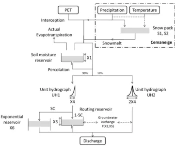
The GR6J model has six parameters to be fitted (Fig. 5): the capacity of soil moisture reservoir (X1) and of the

rout-ing reservoir (X3), the time base of a unit hydrograph (X4),

two parameters of the groundwater exchange function F (X2 and X5), and a coefficient for emptying the

exponen-tial store (X6). The GR6J model is combined here with

the CemaNeige semi-distributed snowmelt runoff component (Valéry et al., 2014). The catchment is divided into five alti-tudinal bands of equal area on which snowmelt and snow accumulation processes are represented. For each band, daily meteorological inputs – including solid fractions of precipita-tion – are extrapolated using elevaprecipita-tion as a covariate, and the snow routine is calculated separately. Finally, its outputs are then aggregated at the catchment scale to feed GR6J. The two parameters of CemaNeige, S1and S2, control the snowpack

inertia and the snowmelt, respectively. S1is used to compute

the thermal state of the snowpack eTG, which is an equivalent to the internal snowpack temperature (◦C). eTG(t ) at day t is a weighted linear combination of the value of eTG(t − 1) (×S1) and the air temperature at the day t (×(1 − S1)). S2is

the snowmelt degree-day factor used to calculate the daily snowmelt depth by multiplying the air temperature when it exceeds 0◦C, with S2. The splitting coefficient (SC) of

effec-tive rainfall between the two stores (in Fig. 5) has been fixed to 0.4 by Pushpalatha et al. (2011), since calibrating the SC leads to only slightly better performance. The allocation of the outflow from the soil moisture reservoir, with 90 % being percolation and 10 % being surface and sub-surface runoff in

Figure 5. Schematic of the rainfall–runoff model GR6J combined with the CemaNeige snowmelt runoff component (after Pushpalatha et al., 2011).

the GR6J model, is the result of previous studies. The GR6J model was selected for its good performance across a large spectrum of river flow regimes (e.g. Hublart et al., 2016; Pon-celet et al., 2017).

No routine to simulate water management (e.g. reservoir) was considered here, since discharges of the 106 gauging sta-tions are weakly altered by human acsta-tions or naturalized dis-charges (i.e. flows corrected from the effects of water use). The eight parameters (six from the GR6J model and two

from the CemaNeige module) were calibrated against the observed discharges using the baseline Safran reanalysis as input data and the Kling–Gupta efficiency criterion (Gupta et al., 2009) KGESQRT calculated on the square root of the

daily discharges as an objective function. The KGESQRT

cri-terion was used to place less emphasis on extreme flows (both low and high flows). As the climate sensitivity space includes unprecedented climate conditions (including colder climate conditions around the current-day condition), the Ce-maNeige module was run for all the 106 catchments, even for those not currently influenced by snow.

The two-step procedure suggested by Caillouet et al. (2017) was adopted for the calibration: first the eight free parameters were fitted only for the catchments significantly influenced by snowmelt processes – i.e. when the proportion of snowfall to total precipitation less than 10 % – and second, for the other catchments, the medians of the CemaNeige pa-rameters were fixed, and the six remaining papa-rameters were then calibrated. Calibration is carried out over the period 1 January 1973 to 30 September 2006, with a 3-year spin-up period to limit the influence of reservoir initialization on the calibration results. The criterion KGESQRT and the

Nash–Sutcliffe efficiency criterion on the log-transformed discharge NSELOG (Nash and Sutcliffe, 1970) were

calcu-lated over the whole period 1958–2013 for the subset of 15 evaluation catchments (Table 1), showing KGESQRTand

NSELOGvalues are above 0.80 and 0.70, respectively. These

two goodness-of-fit statistics indicate that GR6J adequately reproduces observed river flow regime, from low- to high-flow conditions. The less satisfactory performances of GR6J are observed for the Tarn and Roizonne river basins, both characterized by smallest drainage areas and highest eleva-tions of the dataset. These lowest performances are likely to be linked to their location in mountainous areas (snowmelt processes are difficult to reproduce) and to their size (the grid resolution of the baseline climatology fails to capture the cli-mate variability in the headwaters).

4.3 The water-restriction-level modelling framework The WRL modelling framework developed aims to identify periods when the hydrological monitoring indicator is con-sistent with legally binding water restrictions. Only physical components (mainly hydrological drought severity) leading to WR decisions are considered, with no sociopolitical factor accounted for to model water restrictions.

To enable comparison of results across all catchments – in particular to combine response surfaces obtained from differ-ent catchmdiffer-ents (see Sect. 5.1) – the same drought-monitoring indicators and regulatory thresholds were adopted in all the catchments (see Sect. 3 for details), selected as the most commonly used in the 28 DMPs across the RM district, specifically choosing VC3as a monitoring indicator and

10d-VCN3(T )with return periods T of 2, 5, 10 and 20 years as

regulatory thresholds. Each regulatory threshold is defined

for a 10 d calendar period between 1 April and 31 October, resulting in 21 sets of four thresholds. Water restrictions are decided after consulting drought committees that convene ir-regularly depending on hydrological conditions over a time window, i.e. the last N days. Here a time window for analysis of N = 10 d was decided, which is consistent with the prefec-tural decision-making time frame (frequency of updates in water-restriction statements). The WRL modelling time step is finally fixed to 10 d, and a representative value of WRL is given to the twenty-one 10 d calendar periods from April to October. Thus WRL is thus computed as follows:

– VC3(t )is computed from daily discharge Qdaily(t )every

day t .

– VC3(t ) is compared to the corresponding regulatory

thresholds to create time series of daily water-restriction level “wrl”, with wrl(t ) ranging from 0 (no alert) to 3 (crisis): – If 10d-V CN3(2) ≥ VC3(t ) >10d-V CN3(5), wrl(t ) = 0. – If 10d-V CN3(5) ≥ VC3(t ) >10d-V CN3(10), wrl(t ) = 1. – If 10d-V CN3(10) ≥ VC3(t ) >10d-V CN3(20), wrl(t ) = 2. – If 10d-V CN3(20) ≥ VC3(t ), wrl(t ) = 3.

– A WRL(d) time series is created as the median of wrl(t) for each 10 d period.

– The WRL(d) value is set to zero if preceding 10 d pre-cipitation total exceeds 70 % of inter-annual precipita-tion average (precipitaprecipita-tion correcprecipita-tion).

Inputs of the WRL model are daily discharges and precip-itation. Outputs are WRL time series with values for each twenty-one 10 d calendar period from April to October. Mod-elling is only applied to the period April–October, the irriga-tion period and when most water restricirriga-tions are put in place. The low-flow monitoring indicator VC3 and the regulatory

thresholds 10d-VCN3(T )are computed from daily discharge

time series Qdaily based on full period of records prior to

31 December 2013. The log-normal distribution is used to assess the return periods.

The WRL modelling framework can be applied to both ob-served and simulated time series. For the latter, outputs from GR6J are used for simulations under current and modified climate conditions. Regulatory thresholds are derived from simulated discharge using the Safran baseline meteorologi-cal reanalysis as input to moderate the possible effect of bias in rainfall–runoff modelling.

The WRL modelling framework was verified in the 15 evaluation catchments (Table 1). WRL simulations based on modelled (hereafter GR6J) and observed (hereafter HY-DRO) discharge were compared graphically to official

Figure 6. Observed and simulated water-restriction levels considering the two sources of discharge data, GR6J and HYDRO, for each of the 15 evaluation catchments (Table 1). The x abscissa is divided into 10 d periods for each year, spanning the period April–October. Black segments identify updated DMPs.

Table 4. Contingency table for legally binding water restriction (WR∗).

WR∗event WRL ≥ 1 (benchmark) Yes No

WRL ≥ 1 (prediction) Yes Hits False alarms No Misses Correct negatives

WR measures (OBS). A further assessment was conducted using the Sensitivity and Specificity scores (Jolliffe and Stephenson, 2003) to examine how well the WRL modelling framework can discriminate WR severity levels (Table 4). The Sensitivity score assesses the probability of event detec-tion; the Specificity score calculates the proportion of “no” events that are correctly identified. An event was defined as any legally binding water restriction of at least level 1, and a “non-event” was described as a period where WRL is zero or without WR. Comparisons were made over the 2005– 2013 period, corresponding to the common period of avail-ability for OBS, HYDRO and GR6J.

Figure 6 shows years with severe simulated WRLs (e.g. 2005 and 2011) and years with no or few simulated WRs (e.g. 2010 and 2013). Both GR6J and HYDRO simulations are generally consistent with OBS, even if misses are found

(e.g. basins 9 to 11 during the year 2005). There is no system-atic bias, with some overestimations (e.g. 2005 using GR6J in basins 1 and 15; 2007 using HYDRO in basin 15), under-estimations (e.g. 2009 in basin 6–8) and misses (e.g. 2005 us-ing HYDRO in basin 1).

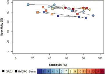
Sensitivity and Specificity scores computed with OBS considered to be a benchmark (Fig. 7) show a large variation across the catchments, in particular for Sensitivity. Speci-ficity scores are around 0.85 for both GR6J and HYDRO, suggesting that more than 85 % of the observed non-events were correctly simulated by the WRL modelling frame-work. The median of WRL Sensitivity score with HYDRO is around 45 %, indicating that for half the catchments, fewer than 45 % of observed events are detected based on HY-DRO discharges, but this increases to 68 % of events de-tected when WRLs are simulated based on GR6J discharge. Using GR6J is more effective for detecting legally binding restriction than using observed discharges, while it is less ef-ficient for predicting periods without restriction for most of the catchments. There is a compensatory effect, which is not easy to detect graphically, since Sensitivity scores are more sensitive than Specificity scores due to the reduced number of observed days with adopted restrictions. No evidence of systematic bias associated with catchment location or river flow regime was found: northern (blue) and southern (red)

Figure 7. Skill scores obtained for the WRL model over the pe-riod 2005–2013. Each segment is related to one of the 15 catch-ments listed in Table 2. The endpoints refer to the source of dis-charge data (GR6J or HYDRO).

catchments are uniformly distributed in the Sensitivity and Specificity space.

Sensitivity and Specificity scores using HYDRO as a benchmark in the contingency table were also used to com-pare simulations from GR6J discharge with those obtained from HYDRO discharge. Median values reach 84 % (Sen-sitivity) and 92 % (Specificity), showing high consistency between HYDRO and GR6J. No statistical link between the hydrological model and WRL model performance was found, with R2between NSELOGand Sensitivity or NSELOG

and Specificity lower than 7 %. In addition, the similar skill scores of GR6J and HYDRO modelling suggest that possible biases in rainfall–runoff modelling does not impact on the ability of the WRL modelling framework to correctly simu-late declared or undeclared WRs.

Choosing the same definitions for the monitoring indica-tor and regulaindica-tory thresholds is a simplifying assumption and may partly explain the deviations between simulated (HY-DRO or GR6J) and adopted (HY(HY-DRO) WR measures. Before stating for VC3 and 10d-VCN3the four prevalent modalities

found in the current DMPs have been tested to reproduce the observed WR, and results have shown weak variables consid-ered in the WR modelling framework. The mains reasons are that all the indicators and thresholds are derived from Qdaily

time series and are highly correlated and thus share, above all, the same information on the dynamics and on the sever-ity of drought.

Heterogeneity in basin characteristics and rules imposed by the DMPs should not result in a systematic difference in the Sensitivity and Specificity score between GR6J and HYDRO identified for most of the 15 evaluation catchments. Simulations were made on near-pristine catchments, and thus water uses are unlikely to be the main reason. Other causes of higher Sensitivity scores obtained when simulated

dis-charges are used as input have been investigated in the WRL modelling framework. However, results of this analysis have not been conclusive. The aforementioned tests with the four prevalent modalities have all led to a higher Sensitivity score using GR6J and a higher Specificity score using HYDRO, demonstrating that the choice of the monitoring indicator and regulatory thresholds is probably not involved. A “smooth-ing” introduced by the hydrological modelling was also sus-pected, but autocorrelation in observed and GR6J-simulated VC3 time series was found to be very similar. Future works

may reinvestigate these aspects. They will need to explore new aspects (e.g. the way WRL is derived from the daily values wrl for each 10 d period) using a longer verification period with a not necessarily uniform but fixed regulatory framework. Indeed some catchments have experienced only 3 years with legally binding water restrictions and DMPs were frequent during the 2005–2013 period (see the black vertical segments in Fig. 6).

Discrepancy between simulated and adopted WR mea-sures is most likely due to the other factors involved in the decision-making process. When regulatory thresholds are crossed, restrictive measures should follow the DMPs. In re-ality, the measures are not automatically imposed but are the result of a negotiating process. This process includes for example some expert-judgment factors such as (i) the evolution of low-flow monitoring indicators and thresholds over the years – e.g. annual revision for the Ouche and irregular revision for the Isère (38), Gard (30), Alpes-de-Haute-Provence (04) and Lozère (48) departments (last one in 2012); (ii) the role of drought committees in negotiating a delay in WRL applications to limit economic damages or to harmonize responses across different administrative sectors sharing the same water intake; and (iii) the local expertise, especially regarding the uncertainty in flow measurements (Barbier et al., 2007) impacting the low-flow monitoring in-dicators, e.g. Côte d’Or (21) and Lozère (48) in the northern and southwestern parts of the RM district, respectively. Note that where WR decisions are not uniquely based on hydro-logical indicators but also involve a negotiation process, the results of the WRL modelling framework should be inter-preted as potential hydrological conditions for stating water restrictions.

Results of our sample study on 15 evaluation catchments show deviations for most catchments but links between order restrictions and hydrological drought severity. These devia-tions may partly be attributed to the use of the same moni-toring indicator and regulatory thresholds across the catch-ments in the modelling (whilst it is not true in reality) as a necessary assumption for a regional-scale analysis. Tests with QC7 as low-flow monitoring variable combined with

the two dominant modalities for the regulatory thresholds show a weak sensitivity of the WRL modelling skill to the choice of the indicators (with a slight increase in Specificity score – ∼ 90 % – while the Sensitivity score is reduced – <50 % – using GR6J). Whilst the developed WRL

mod-elling framework does not account for the expert decision made by drought committees – and hence is not designed to simulate the exact WR decisions – its ability to simulate 68 % of the stated restrictions over the period 2005–2013 demonstrates its usefulness as a tool to objectively simulate the potential of drought restrictions based on hydrological drought physical processes. The methodology was applied to the 106 catchments of the RM district under climate pertur-bations to assess the potential impact of climate change on water restriction in the region. The resulting analysis focuses on water-restriction level higher than 1, denoted thereafter as WR∗.

4.4 The generation of perturbed climate conditions The generation of climate response surfaces relies on syn-thetic climate time series representative of each explore cli-mate condition and used as input to the impact modelling chain (here hydrological model and WRL modelling frame-work). Methods based on stochastic weather simulation have been used (Steinschneider and Brown, 2013; Cipriani et al., 2014; Guo et al., 2016, 2017), but it can be complex to ap-ply them in a region with such a heterogeneous climate as the RM district. Alternatively, the simple “delta-change” method (Arnell, 2003) has been commonly used to provide a set of perturbed climates in a scenario-neutral approach (Paton et al., 2013; Singh et al., 2014) and was used here, similar to Prudhomme et al. (2010, 2013a, b, 2015).

Following Prudhomme et al. (2015), monthly correction factors 1P and 1T are calculated using single-phase har-monic functions: 1P (i) = P0+AP·cos h (i − ϕP) · π 6 i , (1) 1T (i) = T0+AT ·cos h (i − ϕT) · π 6 i , (2)

with P0 and T0 as mean annual changes in precipitation

(Eq. 1) and temperature (Eq. 2), respectively, i as the indica-tor of the month (from 1 to 12), ϕ as the phase parameter, and Aas the semi-amplitude of change (e.g. half the difference between highest and lowest values) for precipitation (Eq. 1) and temperature (Eq. 2). These correction factors were ap-plied to the baseline climate datasets to create perturbed daily forcings:

P∗(d) = P (d) · [PM(month(d)) + 1P (month(d))]/

PM(month(d)), (3)

T∗(d) = T (d) + 1T (month(d)), (4) with P (d) and T (d) representing baseline precipitation and temperature values for day d, P∗(d) and T∗(d) repre-senting the corrected (or perturbed) values for day d, and

¯

PM(month(d)) representing average monthly baseline pre-cipitation for month(d). Corrected potential evapotranspira-tion PET∗time series were derived from temperature values using the formula suggested by Oudin et al. (2005):

PET∗(d) =max[PET(d) + Ra 28.5

1T (month(d))

100 ;0], (5) with PET(d) as baseline potential evapotranspiration values for day d; Ra is the extraterrestrial global radiation for the catchment.

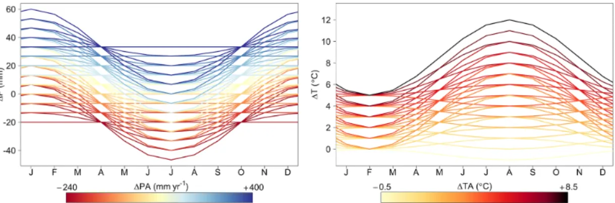
The baseline climate (precipitation and temperature) time series were extracted from the Safran reanalysis over the pe-riod 1958–2013 (56 years), and perturbed time series were generated for the same length. The range of climate change factors to generate the perturbed series were chosen to en-compass both the range and the seasonality of RCM-based (RCM – regional climate model) changes in projections in France. A set of 45 precipitation and 30 temperature scenar-ios was created (Fig. 8), spanning the range of potential fu-ture climate suggested by Terray and Boé (2013) and com-bined independently, resulting in a total of 1350 precipitation and temperature perturbations pairs used to define the climate sensitivity space. In this application, the following applies:

– P0(mm) = −20 + 20/3 × (j − 1), j = 1, . . . , 9,

– AP (mm) = 20/3 × (j − 1), j = 1, . . . , 5,

– T (◦C) = j − 1, j = 1, . . . , 6,

– AT (◦C) = −0.5 + 2 × (j − 1), j = 1, . . . , 5,

– ϕP parameter is fixed to 1 to consider minimum change

in January and maximum change in July, and – ϕT is fixed to 2 to get maximum change in August.

4.5 The assumptions on water uses

Water uses and the feedbacks between use and available re-sources are not explicitly addressed in this application either under current or future conditions. This should not be consid-ered to be a limitation for basins where hydrological mod-elling has been implemented. Indeed, the 106 basins under study have been carefully chosen, since they are currently in-fluenced little or are not inin-fluenced by human actions. These catchments are benchmark catchments where natural water availability is monitored for the statement of restriction or-ders. Water can be abstracted from other neighbouring rivers. Water needs will probably evolve in the coming decades. The water requirement for irrigation may increase parallel to air temperature or may decrease due to adaptive actions (e.g. farmers may choose to plant specific crops less sensi-tive to water shortages). Water needs and sensitivity to wa-ter restrictions depend on socio-economic and institutional pathways. Forward-looking studies have been recently car-ried out with the involvement of local experts but at the local scale (Grouillet et al., 2015 for the Hérault river basin; An-drews and Sauquet, 2017 for the Durance river basin). The distinct underlying assumptions make it difficult to combine

Figure 8. Monthly perturbation factors 1P and 1T associated with the climate sensitivity domain. The colour of the line is related to the intensity of the annual change 1P A and 1T A.

and to extend the prospective scenarios over the RM district. Thus, the water-restriction modelling framework considers, in this application, the “business-as-usual” scenario, which assumes that only minor change in water demand behaviour will occur. In particular, no major alteration of the river flow regime is projected for the 106 catchments. Despite being unrealistic, maintaining the current conditions allows for the assessment of the impact of climate change regardless of any other human-induced changes. The advantage is that results are easier to understand and to embrace by stakeholders than those obtained with complex multi-sectorial scenarios that they may not identify with.

5 Drought management plans under climate change and their impact on irrigation use

5.1 The water-restriction response surfaces

The 1350 sets of perturbed precipitation, temperature and PET time series were each fed into the WRL modelling framework for each of the 106 catchments. Both VC3

(mon-itoring indicators) and 10d-VCN3(T )(regulatory thresholds)

were computed from GR6J 56-year discharge simulations. For each scenario, the number of 10 d periods under a wa-ter restriction of at least level 1 (WR∗) was calculated and expressed as a deviation from the simulated baseline value, 1WR∗, hence removing the effect of any systematic bias from the WRL modelling framework. Results are shown as WR response surfaces built with x and y axes that repre-sent key climate drivers. Because different climate perturba-tion combinaperturba-tions share the same values of the key climate drivers, hence being represented at the same location of the response surface, the median 1WR∗from all relevant com-binations is displayed as a colour gradient, with the standard deviation (SD) of 1WR∗shown as the size of the symbol.

Response surfaces based on different climate variables for x(precipitation) and y (temperature) were generated over the whole or part of the water-restriction period (April to ber – AMJJASO; March to June – MAMJ; and July to

Octo-ber – JASO, the latter coinciding with the highest tempera-tures) and visually inspected to identify the greatest signal pattern, combined with the smallest dispersion around the surface response (i.e. analysis of the median and the maxi-mum of SD values over the grid cells).

The response surfaces are exemplified on three of the 15 evaluation catchments (Table 1, Fig. 9):

– the Argens river basin, along the Mediterranean coast, where severe low flows occur in summer and actual evapotranspiration is limited by water availability in the soil;

– the Ouche river basin, in the northern part of the RM district, a typical pluvial river flow regime under oceanic climate influences where runoff generation is less bounded by evapotranspiration processes;

– the Roizonne river basin, in the Alps, typical of sum-mer flow regime controlled by snowmelt, with spring to summer climate conditions dominating changes in low flows.

The visual inspection of response surfaces shows the follow-ing:

– 1WR∗ _{is differently driven by the changes in}

precip-itation 1P and in temperature 1T : 1WR∗ _{is very}

sensitive to 1P in the Argens river basin (horizontal stratification in the response surface) and to 1T in the Roizonne river basin (vertical stratification in the re-sponse surface) whilst being controlled by both drivers in the Ouche river basin.

– There is a high likelihood of an increase in the dura-tion of water restricdura-tion in the Roizonne river basin, as shown by a response surface dominated by positive 1WR∗_.

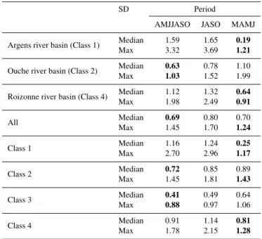
– SD values may vary significantly from one graph to another (Table 5). For both the Argens and Roizonne

Table 5. Summary statistics for standard deviation (SD) of the grid for different axes. Best results are in bold characters.

SD Period

AMJJASO JASO MAMJ

Argens river basin (Class 1) Median 1.59 1.65 0.19

Max 3.32 3.69 1.21

Ouche river basin (Class 2) Median 0.63 0.78 1.10

Max 1.03 1.52 1.99

Roizonne river basin (Class 4) Median 1.12 1.32 0.64

Max 1.98 2.49 0.91 All Median 0.69 0.80 0.70 Max 1.45 1.70 1.24 Class 1 Median 1.16 1.24 0.25 Max 2.70 2.96 1.17 Class 2 Median 0.72 0.85 0.89 Max 1.45 1.81 1.43 Class 3 Median 0.41 0.49 0.64 Max 0.88 0.97 1.06 Class 4 Median 0.91 1.14 0.81 Max 1.78 2.15 1.28

river basins, the largest SDs are found when the re-sponse surfaces are displayed with climate variables computed over the whole period April–October (AMJ-JASO), while smallest SDs are associated with 1P and 1T drivers from March to June. Changes in mean spring to early summer precipitation and temperature mainly govern changes in WR∗ for these two basins. Conversely changes in precipitation 1P and tempera-ture 1T over the full period April–October seem to be the dominant drivers of changes in WR∗for the Ouche river basin.

5.2 Response surface analysis at the regional scale Following Köplin et al. (2012) and Prudhomme et al. (2013a), the 106 response surfaces were classified to define typical response surfaces, designed as tools to help in pri-oritizing actions for adapting water management rules to fu-ture climate conditions in the RM district. Here a hierarchical clustering based on Ward’s minimum variance method and Euclidian distance as similarity criteria (Ward Jr., 1963) was applied, and four classes were identified after inspection of the agglomeration schedule and silhouette plots (Rousseeuw, 1987). A manual reclassification was conducted for the few catchments with negative individual silhouette coefficients to ensure higher intra-class homogeneity. For each class, a mean response surface and associated SD were computed, and main climate drivers associated with WR changes were identified (Table 5).

All suggest an increase in the occurrence of legally bind-ing water restrictions when precipitation decreases or when temperature increases (Fig. 10). An additional temperature

increase and its associated PET increase can compensate for precipitation increase and lead to a decrease in 1WR∗_{, with}

intra-class differences emerging in the magnitude of changes. The identified four typical water restriction response surfaces show a weak regional pattern and common features. Class 4 (including the Roizonne river basin) regroups snowmelt-fed river flow regimes in the Alps, whilst basins of Class 1 are mainly Mediterranean river flow regimes. Class 2 (including the Ouche river basin) and Class 3 catchments are partly in-fluenced by both precipitation and temperature, with 1WR∗ in Class 2 catchments being less sensitive to climatic changes (flatter WR response surface) than catchments of Class 3. The flow regime of Class 2 to 3 ranges from rainfall-fed regimes with high flow in winter and low flow in summer in the northern part of the RM district to regimes partly in-fluenced by snowmelt, with high flows in spring in the Alps and in the Cevennes.

To further the regional analysis and help sensitivity assess-ment at unmodelled catchassess-ments, basin descriptors were in-vestigated as possible discriminators of the four classes. A set of potential discriminators – which included measures of the severity, frequency, duration, timing and rate of change in low-flow events (Table 6); the drainage area and the me-dian elevation for the catchment; and one climate descriptor (mean annual precipitation and mean annual potential evap-otranspiration used to compute an aridity index – AI) – were introduced in a CART model (Classification And Regression Trees; Breiman et al., 1984), aimed at performing succes-sive binary splits of a given dataset according to decision variables. Through a set of “if–then” logical conditions the algorithm automatically identifies the best possible predic-tors of group membership, starting from the most discrim-inating decision variable to the less important factors. The optimal choices are fixed recursively by increasing the ho-mogeneity within the two resulting clusters. At each step, one of the clusters (node) is divided into two non-overlapping parts. Here, to free results from catchment size influence, de-scriptors related to severity were expressed in millimetres per year, millimetres per month or millimetres per day.

Results show three top discriminators, with the aridity in-dex being the strongest:

– the AI given by the mean annual precipitation divided by the mean annual potential evapotranspiration (UNEP, 1993),

– the base-flow index (BFI), a measure of the proportion of the base-flow component to the total river flow, calcu-lated by the separation algorithm separation suggested by Lyne and Hollick (1979),

– the concavity index (CI; Sauquet and Catalogne, 2011) to characterize the contrast between low-flow and high-flow regimes derived from quantiles of the high-flow duration curve.

Figure 9. Climate response surface of legally binding water-restriction-level anomalies 1WR∗for the Argens, Ouche and Roizonne river basins. Each graph is obtained considering changes in mean precipitation 1P and temperature 1T over a specific period as x and y axis.

CART overall misclassification (18 %) suggests a satisfac-tory performance in the classification method, characterized by a parsimonious algorithm (five nodes and three variables) with the potential for a first-guess assessment of the WR re-sponse to disruptions and evaluation of the robustness of ex-isting water restriction at the department-level scale. For each class, Fig. 11 shows the empirical distribution of the three main discriminators, the mean timing θ of daily discharge below Q95 and its dispersion r, which is based on circular

statistics, where Q95 is the 95th quantile derived from the

flow duration curve.

The classification discriminates catchments primarily on the seasonality of low-flow conditions and the aridity index, with the extreme classes (1 and 4) being particularly well discriminated.

Geographically, Class 1 catchments are mainly located along the Mediterranean coast and include the Argens river basin; 1WR∗ is mainly driven by changes in precipitation in spring and early summer. Class 1 gathers water-limited basins with small values of the AI and a weak sensitivity to

climate change in summer. In these dry water-limited basins, the mid-year period exhibits the minimal ratio P / PET, and changes in summer precipitation have hence only a mod-erate impact on low flows; spring is the only season when PET changes are likely to result in both actual evapotran-spiration and discharge changes. WRLs are more likely con-trolled by antecedent soil moisture conditions in spring and early summer. This behaviour is typical of the basins under Mediterranean conditions and was discussed in the context of a scenario-neutral study in Australia (Guo et al., 2016). For those catchments, climate drivers computed in spring (over the period MAMJ) are used to describe the x and y axes of the response surface, fully consistent with water-limited basin processes.

Catchments of both Class 2 and 3 have a similar CI, hence suggesting that flow variability is not a proxy for low-flow re-sponse to climatic deviation. However, BFI values for Class 3 are lower than for Class 2, while Class 3 is characterized by high values for the AI. Despite higher capability to sustain low flows (see BFI values) the response surface

representa-Figure 10. Results of the hierarchical cluster analysis applied to the climate response surface WR∗-level anomalies 1WR∗. Table 6. Hydrological metrics considered to investigate similarity in CART.

Component of the Hydrological indices river flow regime

Severity

Flow exceeded 95 % of the time (Q95).

Annual minimum 10 d daily mean low flow with a 5-year recurrence interval. Annual maximum deficit below threshold Q95exceeded 20 % of time.

Duration

Annual maximum maximal duration of the continuous sequence of zero flow within the year, exceeded on average. every 5 years (D80). Maximum duration of consecutive zero flows (D) are sampled by block maximum approach,

and D80is defined as the empirical 80th percentile of cumulative distribution function of D.

Seasonal recession timescales (DTand Drec). This duration is based on the hydrograph defined by the 1 and 30 d

moving average of the 365 long-term mean daily discharges, d = 1, . . . , 365 (Qdand Q30 d, respectively). Drecis

defined by the time lapse between the median Qd 50and the 90th quantile Qd 90of Qdon the falling limb of the

hydrograph defined by Q30 dand DT=ln(Qd 50/Qd 90)/Drec.

Rate of change

Ratio Q95/Q50.

Concavity index derived from flow duration curve (Q10−Q99)/(Q1−Q99)(Sauquet and Catalogne, 2011). This

descriptor is a dimensionless measure of the contrast between low-flow and high-flow regimes derived from quantiles of the flow duration curve.

Baseflow index (BFI). BFI is a measure of the proportion of the base-flow component to the total river flow, calculated by the separation algorithm separation suggested by Lyne and Hollick (1979).

Class of river flow regime based on average monthly runoff pattern defined by Sauquet et al. (2008; between 1 and 12).

Seasonality ratio (SR). SR = Q95AMJJASON/Q95DJFM(SR > 1 for mountainous catchment), with Q95AMJJASONand

Q95DJFMcomputed on seasonal flow duration curves.

Frequency Proportion of years with at least one value below Q95.

Timing

Mean day of first occurrence of flow below Q95.

Mean and dispersion of the occurrence of flows below Q95within the year (θ and r, rsin(θ )and rcos(θ ). These two

variables are circular statistics. Each day i with zero flow is converted into an angle (ti) and represented by a unit

vector with rectangular coordinates (cos(ti); sin(ti)). The mean of the cosines and sines defines a representative

vector. The value for θ is obtained by calculating the inverse tangent of the angle of the mean vector, and the norm of the mean vector provides a measure of the regularity in the dates (a value close to 1 indicates a high

Figure 11. Statistical distribution of the discriminating factors identified by the CART algorithm (a–c) and the mean timing θ of daily discharge below Q95and its dispersion r (d). The boxplots are defined by the first quartile, the median and the third quartile. The whiskers

extend to 1.5 of the interquartile range; open circles indicate outliers. The colour is associated to the membership to one class, and the name of the class is given along the x axis. The coloured areas in (d) are defined by the first quartile and the third quartile of r and θ . Each dot is related to one gauged basin. The dotted lines indicate the start of four meteorological seasons.

tive of Class 2 is more contrasted than that of Class 3; a possi-ble reason could be drier conditions under current conditions (the median of the AI equals 2.5 for Class 3 compared to 1.6 for Class 2). The monthly perturbation factors (see Sect. 5.1) are the same for all the classes, but the changes in relative terms are less significant regarding the current climate condi-tions for Class 3 than for Class 2 and may explain the limited changes in river flow patterns.

Class 4 regroups catchments with low flows in winter and significant snow storage. The BFI values are high, and due to smooth flow duration curves, the CI demonstrates also high values.

5.3 Risk assessment at the basin scale

The risk-based framework has been applied to the irrigation water use, since annual net total water withdrawal for agri-culture purposes is ranked first at the regional scale. Note that in the Rhône–Mediterranean district around 90 % and 10 % of water used for irrigation originates from surface water and groundwater, respectively. To complement water needs irri-gators may also have access to small reservoirs (storage ca-pacity usually less than 1 × 106m3). Most of the reservoirs are filled by surface water in winter and release water later in the following summer. Water restrictions are not imposed to these reservoirs, but it is assumed here that during severe drought events the majority of them are empty, and thus the existence of potential sources auxiliary to surface water on the conclusions has limited influence on the conclusions.

We assumed here that irrigated farming is globally under failure if the duration with limited or suspended abstraction is above a critical threshold Tcthat causes insufficient water

for crops. The catchment or area i will be considered more vulnerable than the catchment or area j if the likelihood of failure (i.e. exceeding Tc) for catchment or area i is more than

the likelihood of failure for catchment or area j . The critical threshold Tc is a value of total number of days with legally

binding water restrictions that needs to be fixed. To move closer to reality and following Simonovic (2010), the value of Tcis based on the analysis of past events. A possible way

to fix Tcis to simulate historic drought events observed

dur-ing the period 2005–2012 and the effects of water restrictions on crop yield and quality and on economic losses. Comput-ing water deficits was considered rather tricky at the farmComput-ing scale – partly due to the high heterogeneity in crop and soil types, watering systems, conveyance efficiencies, etc., across the RM district – and we have investigated the use of “agri-cultural disaster” notifications as proxies to identify the dam-aging conditions instead.

Specifically the agricultural disaster notifications are is-sued by the agriculture ministry following recommendations from the prefecture to each department affected by extreme hydrometeorological events and applied uniformly over the RM district. Whilst the agricultural disaster status is a global index that may mask heterogeneity in crop losses within each department, and that reflects losses related to both agricul-tural and hydrological droughts, it has the advantage of