HAL Id: hal-00260280
https://hal.archives-ouvertes.fr/hal-00260280
Submitted on 18 Feb 2020
HAL is a multi-disciplinary open access
archive for the deposit and dissemination of
sci-entific research documents, whether they are
pub-lished or not. The documents may come from
teaching and research institutions in France or
abroad, or from public or private research centers.
L’archive ouverte pluridisciplinaire HAL, est
destinée au dépôt et à la diffusion de documents
scientifiques de niveau recherche, publiés ou non,
émanant des établissements d’enseignement et de
recherche français ou étrangers, des laboratoires
publics ou privés.
Distributed under a Creative Commons Attribution| 4.0 International License
Flow filling a curved pipe
Hervé Michallet, C. Mathis, P. Maïssa, F. Dias
To cite this version:
Hervé Michallet, C. Mathis, P. Maïssa, F. Dias. Flow filling a curved pipe. Journal of Fluids
Engi-neering, American Society of Mechanical Engineers, 2001, 123 (3), pp.686-691. �10.1115/1.1374442�.
�hal-00260280�
Flow Filling a Curved Pipe
A small scale experiment was designed to study the propagation of the front of a viscous fluid filling a curved pipe. Several Newtonian fluids with different viscosities and a non-Newtonian fluid have been used. The experiments show that there exists a minimum speed for completely filling the pipe, which depends on the parameters of the experiment (di-ameter d and radius of curvature R of the pipe, kinematic viscosity n of the fluid). Appropriate dimensionless numbers are introduced to characterize the flow and optimal filling conditions.Introduction
Prestressed concrete is commonly used in construction. To pre-vent the prestressed strands from any corrosion, a cement solution is generally injected in pipes of complex geometry. The pipe has to be completely filled in order to avoid weak zones in the struc-ture. The aim of the present study is to observe experimentally the propagation of the front of a viscous fluid injected in a curved pipe, in order to understand the reasons for the appearance of unfilled zones. The solution used in construction is composed of cement, water, liquefier, and retarder. It is a non-Newtonian fluid with air bubbles and particles in suspension. As a first step, we mainly focus in this paper on the filling by Newtonian fluids.
Permanent flows in pipes have been widely studied @1#, particu-larly in the case of curved pipes @2–4# and in engineering appli-cations @5,6#. However, pipe flows involving a propagating front or interface remain poorly understood. The problem of an air-water interface propagating in straight inclined pipes has been addressed only recently @7,8#. As stated above, in industrial appli-cations such as construction, the fluid is often mixed with air bubbles and the flow ought to be treated as a slug flow ~see for example @9,10# for recent work on slug flows in pipes!. But the emphasis of the present work is in the propagation of the interface which clearly separates the gas from the liquid.
The front propagation of a perfect fluid in a horizontal pipe was studied by Benjamin @11#. See also the review by Simpson @12# on gravity currents for related studies and Asavenant and Vanden-Broeck @13#. Benjamin analyzed the front in terms of a ‘‘cavity flow’’ displacing a fluid beneath it. The two-dimensional geom-etry is shown in Fig. 1~a! ~Benjamin also considered the case of a circular cross-section!. Note that Benjamin studied only the case where the free surface detaches with an angle of 60 degrees. By applying conservation of mass, momentum, and energy, he found that there is a unique solution, characterized by
U
Agd
5 1 2, uAgh
5A
2 , h d5 1 2,where the meaning of the various symbols is shown in Fig. 1. In other words, the cavity fills half of the box. An experiment was suggested by Benjamin to realize closely this flow. Liquid initially fills a long rectangular box closed at both ends and fixed horizon-tally. One end is then opened, and under the action of gravity the liquid flows out freely from this end. It can be expected that, after
the transient effects of starting have disappeared, the air-filled cavity replacing the volume of the ejected fluid will progress steadily along the box. Observed in a frame of reference travelling with the front of the cavity, the motion of the liquid will appear to be steady, as shown in Fig. 1~a!. If the effects of viscosity and surface tension are neglected, the velocity of the cavity relative to a stationary observer will be U, and, since h5d/2, the liquid will discharge from the open end with the same velocity. In addition to the solution studied by Benjamin, there is also a one-parameter family of solutions in which the free surface detaches from the box tangentially @14#. Such a solution is plotted in Fig. 1~b!. At the exit of the box, the Froude number u(gh)21/2for these
solu-tions is between 1 and A2. The limit A2 corresponds to Ben-jamin’s solution, while the limit 1 corresponds to the vanishing of the cavity. Using conservation of mass, momentum and energy, one finds the relation
u
Agh
5A
d
h. (1)
Unfortunately, simple arguments based on conservation of mass, momentum and energy do not give as much information in the case of a curved channel.
It is nevertheless important to keep in mind that the Froude number prevails to determine the size of the cavity and thus the ability to fill the pipe. This point will be discussed in the section where we consider various dimensionless numbers. Before that, we first describe the manner in which the experiments have been conducted. Then we present and discuss the experimental results. Experimental Setup
The experimental setup is shown in Fig. 2. Gravity acts down-wards. A transparent PVC pipe ~‘‘Tubclair’’! of inner diameter d is curved with a radius R. Different diameters and radii were considered: 0.6<d<2 cm; 5<R<30 cm. The special case of a horizontal straight pipe was also investigated. The fluid was in-jected with a centrifugal pump at a constant mean flow velocity ~noted U).
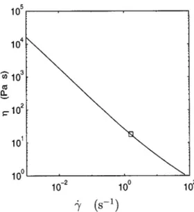
Several fluids were considered in order to investigate the effects of density r, surface tension s, and mainly kinematic viscosity n ~see Table 1!. A series of runs has been performed with a non-Newtonian fluid ~gel!. Its viscosity has been measured with a plane-plane viscosimeter ~see Fig. 3!.
We assume that capillary effects are negligible, so that d@Lc where Lc5s1/2(rg)21/2 is the capillary length (s573 gs22 for water and s521 gs22 for silicone!. In the case of water L
c 50.26 cm and this assumption might be a shortcoming for small diameters. We nevertheless performed a few runs with water con-taminated with wetting agents in order to diminish Lc: the behav-ior and the results were the same within measurements errors. Moreover, the results presented in this paper are limited to d>1 cm.
1Permanent address: Laboratoire des Ecoulements Ge´ophysiques et Industriels
~UJF-INPG-CNRS!, BP53, 38041 Grenoble Cedex 9, Fax: 133 4 76 82 52 71; E-mail: [email protected].
2Corresponding author, present address: Ecole Normale Supe´rieure de Cachan
-CNRS, CMLA UMR8536, 61 avenue du Pre´sident Wilson, 94235 Cachan Cedex; E-mail: [email protected].
H. Michallet
C. Mathis
1P. Maïssa
F. Dias
2Institut Non-Linéaire de Nice, UMR 6618 - CNRS and UNSA, 1361, route des Lucioles, 06560 Valbonne, France
Observations
For a very low flow rate ~a typical mean flow velocity is U ;0.1 cm/s! and a sufficiently large pipe section ~so that d@Lc) the interface is more or less horizontal in the upflow part of the pipe. The flow is dominated by gravity. In the downflow part of the pipe the liquid is creeping down the pipe.
If U is slightly increased, the interface becomes more or less perpendicular to the pipe when rising. At the top, the interface deforms as shown in Fig. 2. The intersection between the interface and the upper part of the pipe ~point C in Fig. 2! is a stagnation point.
If U is increased, the point C moves ~interface in dotted line in Fig. 2!. As soon as U is decreased back to zero, the pipe is emp-tying and the interface moves back to the top.
We consider that the pipe is completely filled when the point C has reached the point B ~Fig. 2!. We define Uc as the critical speed beyond which the interface moves until the pipe is com-pletely filled. The speed v is the mean velocity of the point C moving from A to B ~Fig. 2!: if U is larger than Uc, then v is greater than zero.
For the special case of the non-Newtonian fluid gel, the viscos-ity is smaller where the shear stress is larger, that is near the boundaries. Away from the boundaries, the behavior of the fluid is similar to a solid core pushed by the flow. In other words, the characteristic time of deformation of the interface is very long. Measurements
The mean flow velocity U was obtained by measuring the flow rate in the steady-state regime, i.e., when the pipe was completely filled. The flow rate and v were estimated by measuring the filling time of a graded beaker and the travelling time of point C from A to B ~Fig. 2! with a stopwatch. We may consider that these simple techniques do not lead to any bias error. By repeating the same run ~at least five times! for different flow rates, we have estimated that the precision limit and thus the uncertainty was always better than 10 percent on U and v.
We measured v as a function of U for different experiments using various fluids, pipes, and curvatures ~see Table 1!. In Fig. 4,
vis plotted versus U for several runs in four different
configura-tions. The line v5U delimits the region where physical solutions exist: v cannot be larger than U. In all our experiments v appar-ently varies linearly with U. We may thus determine the critical velocity Uc ~for v50), the slope a5dv/dU and the interfacial velocity v(U50), by rms fitting a straight line into the data for each fluid, pipe diameter and radius of curvature.
Let us first consider the slopea of the four straight lines in Fig. 4. The analysis presented in the Introduction considered a perfect fluid. It was assumed that the flow is identical in a reference frame moving with the front. In this framework, the filling of a pipe is similar to the emptying of the pipe. This would imply thata is equal to one: addingdUto the mean entrance flow velocity would add the same value to the front propagation velocity. It is there-fore not surprising that the slopes of the straight lines in Fig. 4 related to water are close to one. When the fluid is far from perfect
Fig. 1 Steady two-dimensional flow past a cavity. „a… Solution with the free surface leaving the wall with a 60 degree angle. „b… Solution with the free surface leaving the wall tangentially. The point C denotes the detachment point.
Fig. 2 Diagram of the flow and notation. The interface is shown at two different times in solid and dotted lines.
Table 1 Fluids used in the experiments. Density Viscosity Symbol Fluid r~g/cm3) n~cm2/s! R55 cm R530 cm R5` Water 1 0.01 d s ( Water ~40 %! 1 glycerol ~60 %! 1.16 0.086 . , ,• Silicone V50 1 0.5 c x Silicone V100 1 1 n Silicone V300 1 3 v
Gel 1.03 ~See Fig. 3! h
Fig. 3 Dynamic viscosityhof the gel versus the shear stress g˙. Its density isrÄ1.03 gÕcm3. We note that this fluid is very
viscous in the conditions of our experiments „we can estimate roughly thatg˙È2UÕdis less than 10 sÀ1…. Measurements have
been performed with a plane-plane viscosimeter at Ecole des Mines de Paris „CEMEF, Sophia Antipolis….
but still Newtonian ~case of the silicone oil V100 in Fig. 4!,a is clearly smaller than one: when the viscosity is large, the deforma-tion of the front strongly depends on U. For a low viscosity, the deformation of the interface takes place on a very short time scale and the propagation of the front apparently does not depend on the reference frame. In the other limit, that is for a very large viscos-ity, the deformation of the front takes place on a very long time scale and the slope is again close to one ~this is the case of the non-Newtonian fluid!.
The velocity v(0) corresponds to the draining of the pipe. The measurements have been performed by bringing U to zero after filling the pipe: the flow is then from right to left in Fig. 2. It is important to emphasize that v(0) is very small in the case of the non-Newtonian fluid. We have estimated that the draining veloc-ity is about 1 cm per week. The deformation of the front is visible only when the fluid is sheared and Uc is therefore also close to zero for the gel. The agreement in v(0) between the measured values and the values deduced from the fitted straight lines in Fig. 4 is rather good except in the case of water for R530 cm. The discrepancy is probably due to measurement errors but also to wetting effects. The contact between the fluid and the PVC is indeed not the same when filling or emptying the pipe. It was not our purpose to investigate wetting effects and we did not test other materials for the pipe. We therefore have to consider that wetting effects may induce a bias error over Ucof about 10 percent in the worst case, i.e., an uncertainty of 20 percent in the water case.
The critical speed Uc ~mean entrance velocity for which v 50) is plotted against the pipe diameter d in Fig. 5. Uc clearly tends to increase with d. Considering gravitational effects, the larger is d, the more efficient are gravity effects to deform the interface. It is thus not surprising that inertial effects have to be increased to compensate for it. Gravity effects could also reason-ably depend on the radius of curvature. The interface deforms more rapidly when the pipe is curved: for a same diameter, Ucis therefore smaller when R5`. Otherwise, if R is large but not infinite, the travelling time of the front in the pipe is large and the mean entrance velocity has to be large for the front to propagate. In other words, for a very small radius, the front has not enough time to deform before the exit of the pipe. This would explain the fact that Ucis larger for R530 cm than for R55 cm.
In addition, above n51 cm2/s, viscous effects tend to maintain the shape of the interface and thus decrease Uc. This is noticeable
for the silicone V100 and clearly visible for the silicone V300. Again the case of the gel requires specific comments. Uc is very close to zero because the front deforms only when the fluid is sheared as mentioned above. The graphical estimation of Ucgives a nonzero value only for d51.5 cm. This configuration will allow us to estimate dimensionless numbers for the gel in the next section.
The data in Figs 4 and 5 are available in tabular form in Table 2.
Interpretation in Terms of Dimensionless Numbers We may consider various dimensionless numbers that could characterize the flow in our special configuration. Note that in our experiments both the Bond number (Bo5d2rg/s) and the Weber number (We5rdU2/s) are very large: capillary effects are a lot
weaker than inertial and gravitational effects.
Considering inertial and viscous effects in the framework of a curved pipe, we introduce a modified Reynolds number Re, which partly takes into account centrifugal effects, and is in fact the classical Reynolds number plus the Dean number @15#:
Re5Udn
S
11A
RdD
. (2) To balance inertial and gravity effects, we build a modified Froude number Fr, such as:Fr5 U
Agd
S
11A
dR
D
. (3)The modification of the classical dimensionless numbers may be understood by considering that there is a need to add centrifugal effects to maintain the fluid against the concave side of the pipe. Note that ~2! and ~3! tend toward the classical Reynolds and Froude numbers in the limiting case of a straight pipe, i.e., when
Rtends toward infinity.
Let us finally define K, which measures the balance between gravity and viscosity:
K5Re 5Fr
Agd
n 3. (4)Fig. 4 Speed of the front propagationvversus the mean en-trance velocityU„dÄ1.5 cm; see list of symbols in Table 1…. The straight lines are fitted curves by quadratic means.
Fig. 5 Critical speed versus the pipe diameter „see list of symbols in Table 1…
Note that K does not depend on the mean flow velocity U. Re and Fr are computed for U5Ucand plotted against K in Figs. 6 and 7. We may consider two kinds of estimation of the dimensionless numbers for the gel. First we may use the graphical estimation of
Ucfrom Fig. 4 for d51.5 cm: Uc;1.2 cm/s, leading to n;200 cm2/s from Fig. 3 ~assuming that g˙;2Uc/d). This allows us to plot the squares in Figs. 6 and 7. Second, we may estimate from our measurement that Uc;v(0) is nonzero but very small ~six orders of magnitude less than the other values of velocity!. In that case, the squares would be far off the bottom right-hand corners of Figs. 6 and 7. In any case, the gel is possibly following the trend of Newtonian fluids with very large viscosity.
In Fig. 6, the data can be separated into two regions corre-sponding to partially ~below the data! and completely ~above the data! filled pipes. In a situation where the flow is characterized by a point belonging to the border line between the two regions, the filling would be effective over an infinite time, using an infinite amount of fluid. In the frame of a linear approximation, the data follow approximatively the (21) slope, showing that Fr(U 5Uc) is constant from Eq. ~4!.
Another way to represent the same results is given in Fig. 7. One sees that Fr is of the same order of magnitude for all experi-ments while K varies over four orders of magnitude, but Fr is not rigorously constant. In the range of diameters we investigated, we can say roughly that Fr characterizes the ability to fill the pipes
Table 2 Measured values
Fluid Radius of curvature R~cm! Pipe diameter d~cm! Speed of front v~cm/s! Mean entrance velocity U~cm/s! c Silicone V50 5 1.0 28.6 0.0 - 5 1.0 0.6 10.2 - 5 1.0 3.2 14.1 - 5 1.0 11.8 28.7 - 5 1.0 18.9 36.6 - 5 1.2 210.7 0.0 - 5 1.2 4.4 19.8 - 5 1.2 6.7 22.8 - 5 1.2 12.2 31.4 x - 30 1.0 28.8 0.0 - 30 1.0 1.0 13.0 - 30 1.0 4.9 18.9 - 30 1.0 8.9 23.6 - 30 1.0 19.5 35.6 - 30 1.0 22.1 38.4 - 30 1.2 210.8 0.0 - 30 1.2 1.4 19.1 - 30 1.2 4.5 24.0 - 30 1.2 8.9 31.0 - 30 1.2 16.9 43.6 - 30 1.5 213.6 0.0 - 30 1.5 2.2 24.2 - 30 1.5 7.3 34.2 - 30 1.5 16.4 49.2 - 30 1.5 22.5 57.0 - 30 2.0 218.0 0.0 - 30 2.0 2.0 34.6 - 30 2.0 3.4 38.4 - 30 2.0 4.8 41.6 - 30 2.0 6.4 46.3 - 30 2.0 11.2 62.4 D silcone V100 30 1.2 28.5 0.0 - 30 1.2 2.3 14.7 - 30 1.2 2.3 14.7 - 30 1.2 3.9 17.1 - 30 1.2 5.0 18.0 - 30 1.5 211.0 0.0 - 30 1.5 1.3 19.6 - 30 1.5 6.8 29.4 - 30 1.5 10.3 35.3 - 30 1.5 11.8 38.5 v Silicone V300 30 1.5 26.2 0.0 - 30 1.5 0.9 10.5 d water 5 1.0 29.5 0.0 - 5 1.0 3.0 12.4 - 5 1.0 7.2 15.5 - 5 1.0 10.8 18.1 - 5 1.2 210.3 0.0 - 5 1.2 0.7 13.7 - 5 1.2 1.4 14.0 - 5 1.2 7.0 19.1 - 5 1.5 211.9 0.0 s - 30 1.0 29.8 0.0 - 30 1.0 3.2 14.8 - 30 1.0 9.6 19.4 - 30 1.0 13.5 23.1 - 30 1.0 41.3 47.1 - 30 1.2 212.0 0.0 - 0 1.2 0.5 16.9 - 30 1.2 4.6 19.5 - 30 1.2 5.6 22.5 - 30 1.2 9.2 23.2 - 30 1.2 14.1 29.0 - 30 1.2 28.0 42.3 - 30 1.2 28.8 44.9 - 30 1.2 52.7 66.6 - 30 1.5 215.0 0.0 - 30 1.5 9.9 28.9 - 30 1.5 15.0 33.1 - 30 1.5 14.9 33.1 - 30 1.5 22.5 41.1 - 30 1.5 32.6 49.2 - 30 1.5 55.2 72.2 : - ` 1.5 212.0 0.0 - ` 1.5 0.0 9.4 - ` 1.5 0.0 13.3 - ` 1.5 7.1 17.8 - ` 1.5 9.2 20.6 - ` 1.5 13.0 25.2 Table 2 „Continued… Fluid Radius of curvature R~cm! Pipe diameter d~cm! Speed of front v~cm/s! Mean entrance velocity U~cm/s! - ` 1.5 14.1 25.2 - ` 1.5 18.3 29.8 - ` 1.5 20.0 29.8 - ` 1.5 29.0 41.8 - ` 1.5 30.0 41.8 . water ~40%! 1 glyc. ~60%! 5 1.2 1.6 16.7 - 5 1.2 4.8 20.2 - 5 1.2 12.6 27.5 , - 30 1.2 6.1 26.7 - 30 1.2 15.0 38.8 - 30 1.2 14.9 38.8 - 30 1.2 29.5 63.2 - 30 1.2 51.6 95.7 30 2.0 5.7 39.3 - 30 2.0 3.3 42.4 - 30 2.0 10.2 56.8 - 30 2.0 15.2 64.2 - ` 2.0 0.0 6.9 ,• ` 2.0 0.0 8.2 - ` 2.0 16.4 24.8 - ` 2.0 22.7 32.1 - ` 2.0 34.9 47.1 - ` 2.0 45.3 69.2 - ` 2.0 57.0 80.4 h gel 30 1.2 0.0 0.0 - 30 1.2 1.8 2.0 - 30 1.2 20.3 23.1 - 30 1.2 22.3 27.8 - 30 1.5 0.0 0.0 - 30 1.5 6.2 9.3 - 30 1.5 6.5 9.6 - 30 1.5 11.1 15.1 - 30 1.5 13.7 18.5 - 30 1.5 42.3 46.0 - 30 2.0 0.0 0.0 - 30 2.0 38.7 49.6 - 30 2.0 35.9 53.6 - 30 2.0 31.0 55.6 - 30 2.0 44.1 64.0 - 30 2.0 55.9 88.9
~Fr51 corresponds to the theoretical limit ~1! where the flow de-taches tangentially at the exit of a horizontal box, as suggested above in the introduction!. Setting a flow rate leading to Fr>1 would certainly fill any straight pipe.
A careful examination of Fig. 7 leads to several remarks. For Newtonian fluids, the dotted symbols, which correspond to straight pipes, lie below the points corresponding to curved pipes. The latter are gathered with no obvious dependence on the radius of curvature R. Therefore the modified Froude number, which takes into account centrifugal effects, can predict the effective filling of the curved pipes, but is of less interest in the limit of straight pipes. Each group of points corresponds to a different fluid, i.e., viscosity. The tendency for Fr(U5Uc) to increase with
dis clearly visible in each group of points. For K>1022, Fr(U
5Uc) is apparently decreasing with K and the flow would even-tually tend to follow a non Newtonian behavior.
In almost all our experiments, Re is larger than 10 ~see Fig. 6! indicating that viscous effects are smaller than inertial ones. Meanwhile, the data on Fr indicate that both inertial and gravita-tional effects are comparable.
Conclusion
In order to understand the failure in filling curved pipes, we performed a series of experiments using various fluids. We mea-sured the velocity of propagation of the front v and we deduced from its linear dependence with the mean flow velocity U a criti-cal value Uc, below which there is no longer a complete filling of the pipe. This critical velocity Uc is increasing with d for each fluid.
Results are presented in a synthetic way as relations between dimensionless numbers. We have shown, in the scope of our work, that a modified Froude number determines the ability of the flow to fill a curved pipe. In all our experiments and for Newton-ian fluids of different viscosities, the filling was complete for Fr >0.660.2.
We also performed experiments with a non-Newtonian fluid whose rheological behavior is similar to the one of cement sus-pensions. The front deforms very slowly when the shear is weak because this increases the viscosity of the fluid. In that case, the complete filling may be obtained for Fr very small. Following @16,17#, a more extensive study would be needed in order to un-derstand the detail of the non-Newtonian effects.
For industrial applications we advise considering pipes of small diameters and injecting the solution at a relatively low flow rate in order to increase its effective viscosity. However, a future study of interest will be to repeat the present experiments in the context of slug flows.
Acknowledgments
The authors thank C. Peiti at Ecole des Mines de Paris ~CEMEF, Sophia Antipolis! for his help, and R. Leroy and O. Coussy for providing helpful comments. The authors are grateful to J.Ch. Bery for his help in the conception and realization of the experimental apparatus. This study was part of a contract with the Laboratoire Central des Ponts et Chausse´es.
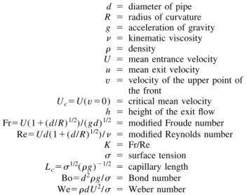
Nomenclature d 5 diameter of pipe R 5 radius of curvature g 5 acceleration of gravity n 5 kinematic viscosity r 5 density
U 5 mean entrance velocity u 5 mean exit velocity
v 5 velocity of the upper point of
the front
Uc5U(v50) 5 critical mean velocity
h 5 height of the exit flow
Fr5U(11(d/R)1/2)/(gd)1/2
5 modified Froude number Re5Ud(11(d/R)1/2)/n 5 modified Reynolds number
K 5 Fr/Re
s 5 surface tension
Lc5s1/2(rg)21/2 5 capillary length Bo5d2rg/s 5 Bond number We5rdU2/s 5 Weber number References
@1# Berger, S. A., Talbot, L., and Yao, L.-S., 1983, ‘‘Flow in curved pipes,’’ Annu. Rev. Fluid Mech., 15, pp. 461–512.
@2# Soh, W. Y., and Berger, S. A., 1984, ‘‘Laminar entrance flow in a curved pipe,’’ J. Fluid Mech., 148, pp. 109–135.
@3# Olson, D. E., and Snyder, B., 1985, ‘‘The upstream scale of flow development in curved circular pipes,’’ J. Fluid Mech., 150, pp. 139–158.
@4# Ishigaki, H., 1994, ‘‘Analogy between laminar flows in curved pipes and or-thogonally rotating pipes,’’ J. Fluid Mech., 268, pp. 133–145.
Fig. 6 Modified Reynolds number „2… computed for UÄUc
versusK„4… „see list of symbols in Table 1.…
Fig. 7 Modified Froude number „3… computed for UÄUc
@5# Popiel, C. O., and van der Merwe, D. F., 1996, ‘‘Friction factor in sine-pipe flow,’’ ASME J. Fluids Eng., 118, pp. 341–345.
@6# Majumdar, B., Mohan, R., Singh, S. M., and Agrawal, D. P., 1998, ‘‘Experi-mental study of flow in a high aspect ratio 90 deg curved diffuser,’’ ASME J. Fluids Eng., 120, pp. 83–89.
@7# Chanson, H., 1997 ‘‘Air-water flows in partially-filled conduits,’’ J. Hydraul. Res. 35, No. 5, pp. 591–602.
@8# Capart, H., Sillen, X., and Zech, Y., 1997, ‘‘The design of sewage sludge pumping systems,’’ J. Hydraul. Res., 35, No. 5, pp. 659–672.
@9# Woods, B. D., and Hanratty, T. J., 1999, ‘‘Influence of Froude number on physical processes determining frequency of slugging in horizontal gas-liquid flows,’’ Int. J. Multiphase Flow, 25, No. 6-7, pp. 1195–1223.
@10# Taitel, Y., Sarica, C., and Brill, J. P., 2000, ‘‘Slug flow modeling for down-ward inclined pipe flow: theoretical considerations,’’ Int. J. Multiphase Flow,
26, No. 5, pp. 833–844.
@11# Benjamin, T. B., 1968, ‘‘Gravity currents and related phenomena,’’ J. Fluid Mech., 31, pp. 209–248.
@12# Simpson, J. E., 1982, ‘‘Gravity currents in the laboratory, atmosphere, and ocean,’’ Annu. Rev. Fluid Mech., 14, pp. 213–234.
@13# Asavenant, J., and Vanden-Broeck, J.-M., 1996, ‘‘Nonlinear free-surface flows emerging from vessels and flows under a sluice gate,’’ J. Austral. Math. Soc., B 38, pp. 63–86.
@14# Vanden-Broeck, J.-M., and Keller, J. B., 1987, ‘‘Weir flows,’’ J. Fluid Mech.,
176, pp. 283–293.
@15# Dean, W. R., 1927, ‘‘Note on the motion of fluid in a curved pipe,’’ Philos. Mag., 20, pp. 208–223.
@16# Chilton, R., Stainsby, R., and Thompson, S., 1996, ‘‘The design of sewage sludge pumping systems,’’ J. Hydraul. Res., 34, No. 3, pp. 395–408. @17# Chilton, R., and Stainsby, R., 1998, ‘‘Pressure loss equations for laminar and
turbulent non-Newtonian pipe flow,’’ J. Hydraul. Eng., 124, No. 5, pp. 522– 529.