HAL Id: hal-00938944
https://hal.archives-ouvertes.fr/hal-00938944
Submitted on 29 Jan 2014
HAL is a multi-disciplinary open access
archive for the deposit and dissemination of
sci-entific research documents, whether they are
pub-lished or not. The documents may come from
teaching and research institutions in France or
abroad, or from public or private research centers.
L’archive ouverte pluridisciplinaire HAL, est
destinée au dépôt et à la diffusion de documents
scientifiques de niveau recherche, publiés ou non,
émanant des établissements d’enseignement et de
recherche français ou étrangers, des laboratoires
publics ou privés.
Adaptive Mesh Reconstruction in X-Ray Tomography
Fanny Buyens, Michele Quinto, Dominique Houzet
To cite this version:
Fanny Buyens, Michele Quinto, Dominique Houzet. Adaptive Mesh Reconstruction in X-Ray
Tomog-raphy. MICCAI 2013 - Workshop on Mesh Processing in Medical Image Analysis, Sep 2013, Nagoya,
Japan. �hal-00938944�
Tomography
Fanny Buyens1, Michele A. Quinto1, and Dominique Houzet2 1
CEA LIST, 91191 Gif sur Yvette, France
2 GIPSA-Lab, Grenoble-INP, 38402 St Martin d’Heres, France
{[email protected],[email protected]}
Abstract. This paper presents an X-ray tomographic reconstruction
method based on an adaptive mesh in order to directly obtain the typical gray level reconstructed image simultaneously with its segmentation. It also leads to reduce the number of unknows throughout the iterations of reconstruction and accelerates the process of algebraic algorithms. The process of reconstruction is no more based on a regular grid of voxels but on a mesh composed of non regular tetraedra that are progressively adapted to the content of the image. Each iteration is composed by two main steps that successively estimate the values of the mesh elements and segment the sample in order to make the grid adapted to the content of the image. The method was applied on numerical and experimental data. The results show that the method provides reliable reconstructions and leads to drastically reduce the memory storage compared to usual reconstructions based on pixel representation.
Keywords: X-ray tomography, mesh representation, level-set
1
Introduction
Tomography reconstruction from projections data is an inverse problem widely used in the medical imaging field. With sufficiently large number of projections over the required angle, the FBP (Filtered Back-Projection) algorithms allow fast and accurate reconstructions. However in the cases of limited views (low dose imaging) and/or limited angle (specific constrains of the setup), the data available for inversion are not complete, then the problem becomes more ill-conditioned and the results show significant artifacts. In these situations, an alternative approach of reconstruction, based on a discrete model of the prob-lem, consists in using an iterative algorithm or a statistical modelisation of the problem to compute an estimate of the unknown object. These methods are clas-sicaly based on a volume discretization into a set of voxels and provide 3D maps of densities. High computation time and memory storage are their main disad-vantages. Moreover, whatever the application is, the volumes are segmented for a quantitative analysis. Numerous methods of segmentation with different inter-pretations of the contours and various minimized energy functions are offered with results that can depend on their use by the application.
During the last decade, several studies focused on new approaches simulta-neously performing reconstruction and segmentation. These methods are based on a modelling of the sample and solve an optimization problem for which the unknown variables are the location of the boundaries and the intensity distribu-tion. Some authors proposed the reconstruction of 3D binary images composed of uniform compact objects totally included in uniform backgrounds [1]. The scene is reconstructed using parametric surface models (splines). The parame-ters are estimated from the data but the final results strongly depend on the initialization. Senasli et al. [2] also proposed to use active contours based on a stochastic process to reconstruct binary images in the context of few data. Us-ing these object-based methods for tomographic reconstruction, Charbonnier [3] proposed to introduce a priori on the shape, to constrain the length of the curve to be appropriated to the estimated object. Yoon et al [4] proposed a simulta-neous segmentation and reconstruction method in the case of limited angle of view in CT. The segmentation and reconstruction are achieved by alternating a segmentation step using the a two-phase level set function and reconstruction step using a conjugate gradient to estimate the intensity value. An initial image obtained after few iterations of the reconstructed algorithm is used to initialize the level set function. The method is performed using usual pixelised grids.
In the framework of SPECT tomography, Brankov et al. proposed a method for 2D tomographic image reconstruction based on an irregular image represen-tation [5]. The mesh is generated from a FDK reconstruction using a feature map extraction performed on a regular pixelized grid. The classical algebraic ML-EM algorithm is then used to proceed the reconstruction on the irregular mesh. Sitek and al. also proposed a method of reconstruction based on a dif-ferent representation of the volume: the domain is here defined by a cloud of points and represented by non overlapping tetraedra defined by these points [6, 7]. From a coarse regular grid, nodes are added to the the point cloud at the locations of large intensity variations during the reconstruction. The method is more complex but strives for a more efficient image representation.
In this context, we propose a method of reconstruction in X-ray tomography that uses a classical iterative algorithm modified to run on an adaptive triangu-lar mesh jointly with a level set method to achieve simultaneous reconstruction and segmentation. This approach provides both the density map of the sample and the segmentation of all the materials that compose the object. The refine-ment of the mesh, relying on the segrefine-mentation, significantly reduces the number of unknowns since the homogeneous regions, containing poor information, are represented by a coarse mesh. No additional post processing steps are required leading to a reliable reproducibility of the process. Besides, the representation of the image by a mesh adapted to its content allows to reduce considerably the memory size of the reconstructed image (reduction of the problem of memory storage) and to deal with highly pixelated detectors.
2
Materials and method
After a step of initialization, the proposed method is composed of three main stages : reconstruction, segmentation and adaptation of the mesh to the object that successively alternate until convergence.
2.1 Initialization
This step consists in generating a first mesh according to the Delaunay’s criteria i.e. a triangulation whose circumscribing circle of any facet of the triangulation contains no vertex in its interior (Delaunay triangulation). All the elements of this initial mesh are initialized with the same non-zero constant value. The number of elements Nt of this first mesh is chosen as 101Ndim < Nt < Ndim
where dim = {2, 3} is the dimension of reconstruction and N = max{Nx, Ny}
with Nx and Ny the number of pixels through the dimensions of the detector.
2.2 Reconstruction
The physics of the radiation determines the nature of the information collected by the detectors of the acquisition system. We consider here the case of X-ray transmission tomography for which every crossed material attenuates the flux of photons according to its nature and its thickness. A difference of intensity is measured in the log scale between the incoming and the outcoming photon flux in the materials which is expressed by the Beer-Lambert law. Discretized, the model is written as following:
p = Hf + ϵ (1)
where f is the vector containing the N discretized values of the object, p is the vector containing the M measurements, ϵ is a vector representing modeling and measurements errors, and H is the M×N projection matrix. M is equal to nproj×
ndet where nproj is the number of projections and ndet the number of detectors.
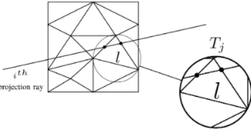
The elements of matrix H represent the contribution of each element of the mesh to the projection rays. As shown in figure 1, the element hi,j corresponds to the
length of the projection ray i intercepted by the element of the mesh j.
Here we investigate a Conjuguate Gradient (CG) optimization algorithm to solve the problem as a least-square estimation. We denote the unknown param-eter as f and the estimation is done by minimizing the cost function J (f ):
ˆ f = arg min f {J(f)} (2) with J (f ) =∥p − Hf∥2 (3)
For quadratic cost functions, the iterative CG algorihtm with an optimal de-scent step is given bellow, with n the indice of the iterations, Nmaxthe maximum
number of iterations, d the CG descent direction and δ the gradient norm toler-ance. gndenotes the gradient of the cost function at the nthiteration gn=
∂J (f ) ∂f .
Fig. 1: The contribution of the element j of matrix H to the projection ray i corresponds to the intercepted length l.
n = 0, d0=−g0
while n < Nmax and norm(gn) < δ
do αn = − gT nd ⟨dn,HTHdn⟩ fn+1 = fn+ αndn β = g T n+1gn+1 gT ngn dn+1 = −gn+1+ βdn n + +
In the above algorithm, the descent step αn is calculated with the goal of
minimizing the cost function for the next iteration in the direction of the descent. This means :
αn= arg min α {J(fn
+ αdn)} (4)
The expression given in the CG algorithm above is the exact solution for eq. 4 while the cost function is quadratic. Even with nonquadratic cost functions, the same strategy can be used to estimate the descent step.
The gradient-based iterative methods of reconstruction require two main steps (a projection and a backprojection) over one iteration [8]. These two main operators are very time consuming. To speed up computation, they were thus implemented on Graphic Process Units (GPU) using a ray-tracing method.
2.3 Segmentation
The step of segmentation is performed after the step of reconstruction. It consists in delineating the boundaries of the object(s) which are used for the mesh refine-ment. The segmentation is performed using the multiple phase level set method. The level set function is defined by an implicit function ϕ(x, t) that moves inRn in relation to time t. The curve described by the interface Γ (t) ={x | ϕ(x, t) = 0} between two regions of the image domain, is determined at time t by zero-level curve of the function ϕ(x, t).
The movement of the curve is defined by the Euler-Lagrange equation :
ϕt+ Vx· ∇ϕ = 0 (5)
where ϕt=∂ϕ∂t and Vx=∂x∂t is the velocity field.
We investigate here the work of [9] and [10] whose segmentation approach is based on convex energies. This Globally Convex Segmentation or GCS formu-lation is based on the observation that the steady state solution of the gradient flow coincides with the steady state of the simplified flow:
∂ϕ ∂t = ( ∇.|∇ϕ|∇ϕ − µ((c1− f)2− (c2− f)2 )) (6) that represents the gradient descent for minimizing the energy:
E(ϕ) =|∇ϕ| + µ < ϕ, r > (7) with r = (c1− f)2− (c2− f)2. The global minima is defined by constraining the
solution in the interval [0,1] resulting in the optimization problem :
min0≤ϕ≤1|∇ϕ| + µ < ϕ, r > (8)
After optimization, the segmented region is found by thresholding the level set function to get :
Γ = x : ϕ(x) > α (9)
In the case of an image composed by only one material, 0≤ ϕ(x) ≤ 1 and α is set to 0.5. More generally, if 0 ≤ ϕ(x) ≤ c, with c ≤ 1 and c = max( ϕ(x)),
α is set to 2c. In the case of an image composed of several materials, the regions are then segmented by setting α to the values corresponding to the valleys of the histogram of the image.
2.4 Refinement
Given the set of points S defining the above segmented boundaries :
S ={xi,j, . . . , xNj,j; . . . ; xi,M, . . . , xNM,M}, x ∈ R
2
(10) where Nj is the number of points of the contour j, and M the number of
seg-mented contours. Since the lengths of the contours are different, the optimal number of points describing each boundary is given by:
K = k· lj lmin
(11) where, lj is the length of contour j, and lminthe length of the smallest contour.
k is empirically set to 100. The mesh is then generated using the functions of
3
Results
The method was implemented and applied in 2D for the reconstruction of a slice of a statistical model of a human knee which is composed of a single material (bone). Secondly, the method was applied on the common Shepp-Logan phantom which is composed of several materials.
3.1 2D Reconstruction of the knee
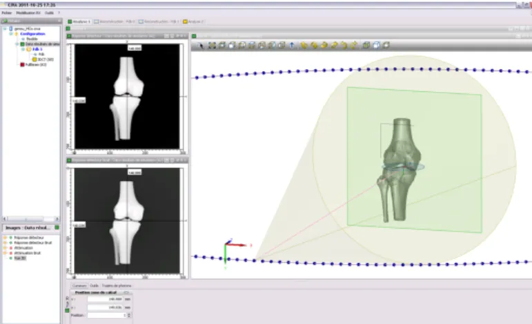
The first studied phantom is a statistical model of the knee only composed by one material (bone). The projections have been computed using the RT-CT module of the CIVA software [12] with a typical configuration of a common radio-graphic exam of the knee: the distance knee - detector is 80 mm and the distance knee - X-ray source 1080 mm. The dimensions of the 2D imaging detector are 151.5mm×151.5mm (with 1024×1024 pixels). Fig 2 shows a 3D representation of the phantom and a snapshot of the simulation scene in CIVA.
In the follow, let’s denote ATM the proposed method for Adaptive Triangular Mesh reconstruction.
Fig. 2:Snapshot of the scene in CIVA software for the simulation of the projections of the phantom showing the 3D phantom of the knee, the detector in green and a part of the trajectory of the X-ray source.
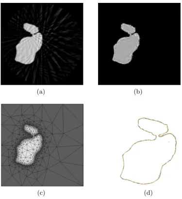
Figure 3 shows the results of 2D reconstructions of a slice of the 3D model of the knee using 36 projections with the FDK algorithm (Fig. 3a) and with the ATM method (Fig. 3b) using α = max(ϕ(x))2 (one material to be segmented). Figure 3c shows the final mesh
Figures 3b and 3c correspond respectively The final image and its correspond-ing final mesh. This latter is composed of 1751 triangles which can be compared to the 1024×1024 pixels (=1048576 pixels) of the FDK reconstruction 3a (about
(a) (b)
(c) (d)
Fig. 3:Reconstructions of a 2D slice of the phantom of the knee using 36 projections with (a) the analytical FDK algorithm, (b) the ATM method - (c) the corresponding irregular mesh of the final ATM image showed in (b) and (d) Comparison of the real contour of the knee (black contour) with the contours obtained from FDK reconstruc-tion followed by a level set segmentareconstruc-tion (green contour) and directly with the ATM method (red contour).
×600 more elements). As Table 1 sums up, if coded on 64 bits (binary), the
pixelized image sizes in memory 8MB while the final irregular meshed image sizes 84KB (ASCII) that is more than hundred times less with in addition the information of segmentation (the mesh images are stored in OFF file format). Figure 3d compares the real shape of the knee (black line) and the level of the central slice with those obtained with FDK reconstruction coupled with an ad-ditional step of level set segmentation (green line), and directly with the ATM method (red line)
3.2 2D Reconstruction of the Shepp-Logan
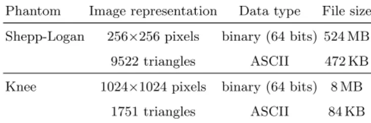
The second phantom is a 2D slice of the Shepp-Logan phantom which is shown in figure 6c. It is composed of several structures whose values range from 0 to 2.0. 256 projections were computed with an analytical projector in the case of a fan-beam configuration. The detector is composed by 256 pixels. Figure 4
shows the reconstructions obtained with 4b FDK algorithm and 4c-4d with ATM method (respectively the finale image and its corresponding triangular mesh) using a set of 360 projections. The mesh was initialized with 65536 triangles and reached 9522 triangles at the end on the process. In this case of several materials, parameter α was set to 0.05, 0.18 and 0.4 in order to segment all the sturctures.
(a) (b)
(c) (d)
(e) (f)
Fig. 4:(a) 2D Shepp-Logan (256x256 pixels) (b) FDK reconstruction, (c) ATM recon-struction and (d) its corresponding final mesh (9522 triangles). (e) ATM reconrecon-struction superimposed with the real contour of the numerical phantom and (f) the centered hor-izontal profiles obtained from FDK and ATM compared with the real one
Figure 4e shows Fig. 4c superimposed with the real contours of the phantom (in red) and Figure 4f shows the profiles obtained from the FDK (red) and ATM (blue) reconstructed images compared with the real one (pink). The ATM profile is quite noiser but
Table 1:Memory storage size of the reconstructed images: pixel representation vs ATM representation
Phantom Image representation Data type File size Shepp-Logan 256×256 pixels binary (64 bits) 524 MB 9522 triangles ASCII 472 KB Knee 1024×1024 pixels binary (64 bits) 8 MB
1751 triangles ASCII 84 KB
Parameters study
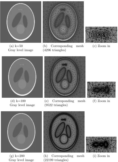
Figure 5 shows the results of 2D reconstructions of the Shepp-Logan phantom when varying the value of parameter k. It shows that this parameter has influence on the definition of small regions. Indeed, when zooming on the top zone of the phantom (images on the right column), we can observe the mesh density increasing with the value of k and therefore a better definition of these three regions. However, the other regions of the phantom (bigger) are not impacted by the variation of k. The value of parameter k has thus to be high when the studied object is composed by small structures.
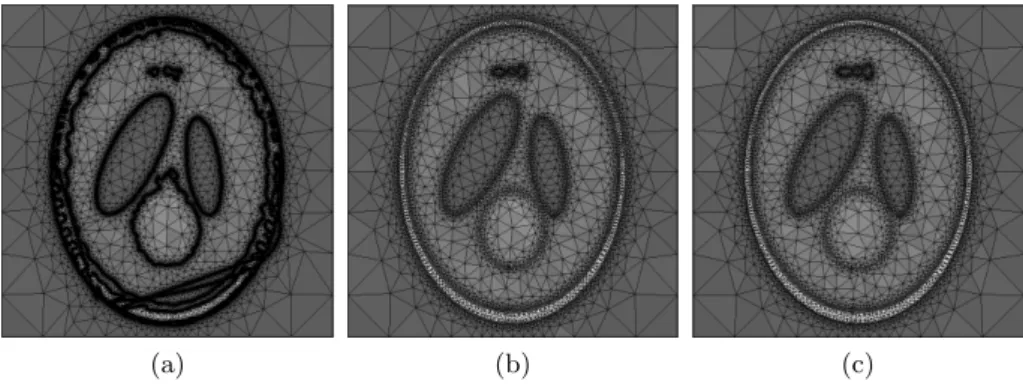
Figure 6 shows the influence of the number of iterations of the first step of reconstruction before segmentation. It shows that a good segmentation of the object is obtained rather fast, between five and ten iterations. The drastic simplication of the mesh generated after segmentation makes the computation faster during the next iterations what speed up the global proposed method.
4
Conclusions and Perspective
The method described in this paper proposes an alternative image representation in the field of image reconstruction in X-ray tomography. The useful pixel image representation (regular grid) can mismatch with the content of the images and is here replaced by an irregular and adaptive mesh. This kind of representation decreases the number of unknowns since the mesh is fine to well describe the contours of the object and its details, and becomes progressively coarse in the homogeneous regions where there is no information.
The method alternatively runs a current algebraic or statistical algorithm adapted to triangular mesh (in particular the main operators of projection and
(a) k=50 Gray level image
(b) Corresponding mesh (4296 triangles)
(c) Zoom in
(d) k=100 Gray level image
(e) Corresponding mesh (9522 triangles)
(f) Zoom in
(g) k=200 Gray level image
(h) Corresponding mesh (22199 triangles)
(i) Zoom in
Fig. 5:Influence of parameter k on the mesh definition and the representation of the image. On the left column (a), (d) and (g) represent the gray level images corresponding to the meshed images (b), (e) and (h) respectively obtained with k=50, k=100 and k=200. On the right column, (c), (f) and (i) images show a zoom of the three little regions at the top of the phantom.
back-projection), a level set method of segmentation and a step of refinement. In this study, the method has been evaluated on 2D numerical data using an
(a) (b) (c)
Fig. 6: Influence of the number of iterations of reconstruction on segmentation and mesh generation : results (a) after 5 iterations, (b) 10 iterations and (c) 15 iterations.
algorithm of conjugate gradient for the reconstruction and a level set approach for the segmentation. The results show that the method provides the common gray level images in addition of a mesh adapted to the content of the images. The mesh is a means to obtain additional information without further image processing tools application. Each segmented region can be easily extracted and studied regardless of the other ones if necessary.
This kind of algorithm could be used for example in the follow up of patholo-gies such as the osteoarthritis of the knee. The mesh could thus be initialized with a previous exam to drastically speed up the reconstruction, and the results could be stored in the informatic file of the patient generating less problems of memory size. Indeed Table 1 shows how this representation is efficient for large reconstruction : it decreases the space memory by a factor 1000 for the storage of a 1024×1024 pixels image.
Since this representation decreases the number of unknowns, the data sets are light and the parallelization of the two main operators does not significantly accelerate the computation time in 2D. The reconstruction of 3D volumes and the use of 2D detector whose number of pixels increases could thus be efficiently treated with this approach.
At present a 3D projector has been implemented on GPU using a 3D ren-dering method used in computer graphics adapted to our iterative process and a quad tree hierarchical structure on each face of the volume of reconstruction to speed up the stage of initilization of the rays.
References
1. C. Soussen and A. Mohammad-Djafari, “Polygonal and polyhedral contour recon-struction in computed tomography,” IEEE Trans. Med. Imag, vol. 13, no. 11, pp. 1507–1523, 2004.
2. M. Senasli, L. Garnero, A. Herment, and E. Mousseaux, “3D reconstruction of vessel lumen from very few angiograms by dynamic contours using a stochastic approach,” Graph. Models, vol. 62, no. 2, pp. 105–127, 2000.
3. P. Charbonnier, “Reconstruction d’images: r´egularisation avec prise en compte des discontinuit´es,” Ph.D. dissertation, University of Nice-Sophia Antiolis, 1994. 4. S. Yoon, A. R. Pineda, and R. Fahrig, “Simultaneous segmentation and
reconstruc-tion: A level set method approach fo limited view computed tomography,” Med.
Phys., vol. 37, no. 5, pp. 2329–2340, 2010.
5. J. G. Brankov, Y. Yang, and M. N. Wernick, “Tomographic image reconstruction based on a content-adaptive mesh model,” IEEE Trans. Med. Imag., vol. 23, no. 2, pp. 202–212, 2004.
6. A. Sitek, R. H. Huesman, and G. T. Gullberg, “Tomographic reconstruction using an adaptive tetrahedral mesh defined by a point cloud,” IEEE Trans. Med. Imag., vol. 25, no. 9, pp. 1172–1179, 2006.
7. N. Pereira and A. Sitek, “An svd based analysis of the noise properties of a point cloud mesh reconstruction method,” IEEE NSS/MIC, pp. 4135–4142, 2011. 8. S. Kawata and O. Nalcioglu, “Constrained iterative reconstruction by the conjugate
gradient method,” IEEE Trans. Med. Imag., vol. MI-4, no. 2, pp. 65–71, 1985. 9. T. Chan and S. E. ans M. Nikolova, “Algorithms for finding global minimizers
of image segmentation and denoising models,” SIAM J. Appl. Math., vol. 66, p. 19321648, 2006.
10. T. GoldStein, X. Bresson, and S. Osher, “Geometric application of the split breg-man method: Segmentation and surface reconstruction,” J. Sci. Comput., vol. 45, no. 1-3, pp. 272–293, 2010.
11. CGAL, “Computational Geometry Algorithms Library,” http://www.cgal.org. 12. CIVA, http://www-civa.cea.fr.