Physiologically Informed Bayesian Analysis of ASL fMRI Data

(1)

HAL Id: hal-01100266

https://hal.inria.fr/hal-01100266

Submitted on 6 Jan 2015

HAL is a multi-disciplinary open access

archive for the deposit and dissemination of

sci-entific research documents, whether they are

pub-lished or not. The documents may come from

teaching and research institutions in France or

abroad, or from public or private research centers.

L’archive ouverte pluridisciplinaire HAL, est

destinée au dépôt et à la diffusion de documents

scientifiques de niveau recherche, publiés ou non,

émanant des établissements d’enseignement et de

recherche français ou étrangers, des laboratoires

publics ou privés.

Physiologically Informed Bayesian Analysis of ASL

fMRI Data

Aina Frau-Pascual, Thomas Vincent, Jennifer Sloboda, Philippe Ciuciu,

Florence Forbes

To cite this version:

Aina Frau-Pascual, Thomas Vincent, Jennifer Sloboda, Philippe Ciuciu, Florence Forbes.

Physiolog-ically Informed Bayesian Analysis of ASL fMRI Data. BAMBI 2014 - First International Workshop

on Bayesian and grAphical Models for Biomedical Imaging, Sep 2014, Boston, United States. pp.37

-48, �10.1007/978-3-319-12289-2_4�. �hal-01100266�

(2)

Abstract. Arterial Spin Labelling (ASL) functional Magnetic Reso-nance Imaging (fMRI) data provides a quantitative measure of blood perfusion, that can be correlated to neuronal activation. In contrast to BOLD measure, it is a direct measure of cerebral blood flow. However, ASL data has a lower SNR and resolution so that the recovery of the per-fusion response of interest suffers from the contamination by a stronger hemodynamic component in the ASL signal. In this work we consider a model of both hemodynamic and perfusion components within the ASL signal. A physiological link between these two components is analyzed and used for a more accurate estimation of the perfusion response func-tion in particular in the usual ASL low SNR condifunc-tions.

1 Introduction

Arterial Spin Labelling (ASL) [1] provides a direct measure of cerebral blood flow (CBF), overcoming one of the most important limitations of Blood Oxygen Level Dependent (BOLD) signal [2]: BOLD contrast cannot quantify cerebral perfusion. In contrast to BOLD, ASL is able to provide a measure of baseline CBF as well as quantitative CBF signal changes in response to stimuli pre-sented to any volunteer in the scanner during an experimental paradigm. Hence, ASL enables the comparison of CBF changes between experiments and subjects (healthy vs patients) making its application to clinics feasible. In addition, ASL signal localization is closer to neural activity. ASL has already been used in clin-ics in steady-state for instance for probing CBF discrepancy in pathologies like Alzheimer’s disease and stroke, but its use in the functional MRI context has been limited so far. Despite ASL advantages, its main limitation lies in its low Signal-to-Noise Ratio (SNR), which, together with its low temporal and spatial resolutions, makes the analysis of such data more challenging.

According to [3, 4], ASL signal has been typically analyzed with a general linear model (GLM) approach, accounting for a BOLD component mixed with the perfusion component. In such a setting both the hemodynamic response function (HRF or BRF for BOLD response function) and perfusion response function (PRF) are assumed to be the same and to fit the canonical BRF shape. In contrast, an adaptation of the Joint-Detection estimation (JDE) framework [5]

(3)

to ASL data has been proposed in [6, 7] to separately estimate BRF and PRF shapes, and implicitly consider the control/label effect which, as stated in [4], increases the sensitivity of the analysis compared to differencing approaches. Al-though this JDE extension provides a good estimate of the BRF, the PRF esti-mation remains much more difficult because of the noisier nature of the perfusion component within the ASL signal. In the past decade, physiological models have been described to explain the physiological changes caused by neural activity. In [8, 9], neural coupling, which maps neural activity to ensuing CBF, and the Balloon model, which relates CBF to BOLD signal, have been introduced. These models describe the process from neural activation to the BOLD measure, and the impact of neural activation on other physiological parameters.

Here, we propose to rely on these physiological models to derive a tractable linear link between perfusion and BOLD components within the ASL signal and to exploit this link as a prior knowledge for the accurate and reliable recovery of the PRF shape in functional ASL data analysis. This way, we refine the separate estimation of the response functions in [6, 7] by taking physiological information into consideration. The structure of this paper goes as follows: the physiological model and its linearization to find the PRF/BRF link are presented in section 2. Starting then from the ASL JDE model described in section 3, we extend the estimation framework to account for the physiological link in section 4. Finally, results on artificial and real data are presented and discussed in sections 5-7.

2 A physiologically informed ASL/BOLD link

Our goal is to derive an approximate physiologically informed relationship be-tween the perfusion and hemodynamic response functions so as to improve their estimation in a JDE framework [6, 7]. We show in this section that, although this relationship is an imperfect link resulting from a linearization, it provides a good approximation and allows to capture important features such as a shift in time-to-peak from one response to another. For a physiologically validated model, we use the extended balloon model described below.

2.1 The extended Balloon model

The Balloon model was first proposed in [10] to link neuronal and vascular pro-cesses by considering the capillary as a balloon that dilates under the effect of blood flow variations. More specifically, the model describes how, after some stimulation, the local blood flow finptq increases and leads to the subsequent

augmentation of the local capillary volume νptq. This incoming blood is strongly oxygenated but only part of the oxygen is consumed. It follows a local decrease of the deoxyhemoglobin concentration ξptq and therefore a BOLD signal variation. The Balloon model was then extended in [8] to include the effect of the neuronal activity uptq on the variation of some auto-regulated flow inducing signal ψptq so as to eventually link neuronal to hemodynamic activity. The global physio-logical model corresponds then to a non-linear system with four state variables

(4)

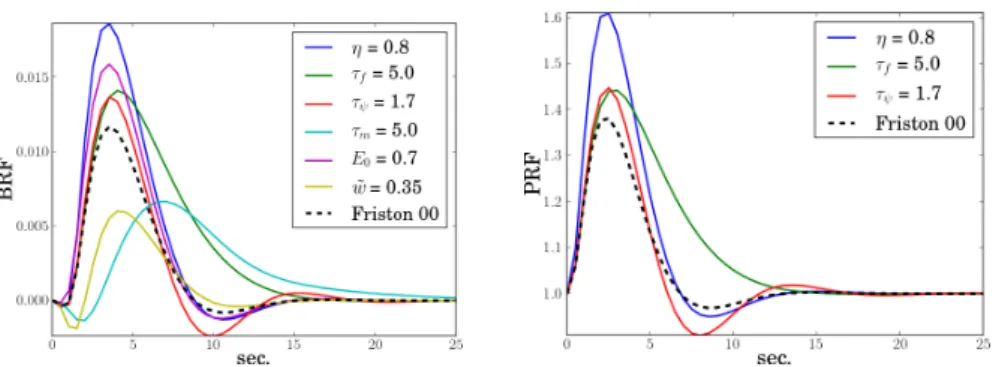
Fig. 1. Effect of the physiological parameters on the BRF (left) and PRF (right) shapes. The parameters values proposed in [8] are used except for one parameter whose identity and value is modified as indicated in the plot.

tψ, fin, ν, ξu corresponding to normalized flow inducing signal, local blood flow,

local capillary volume, and deoxyhemoglobin concentration. Their interactions over time are described by the following system of differential equations:

$ ’ ’ ’ ’ ’ & ’ ’ ’ ’ ’ % dfinptq dt “ ψptq dψptq dt “ ηuptq ´ ψptq τψ ´ finptq´1 τf dξptq dt “ 1 τm ´ finptq1´p1´E0q 1{finptq E0 ´ ξptqνptq 1 ˜ w´1 ¯ dνptq dt “ 1 τm ´ finptq ´ νptq 1 ˜ w ¯ (1)

with initial conditions ψp0q “ 0, finp0q “ νp0q “ ξp0q “ 1. Lower case notation

is used for normalized functions by convention. The system depends on 5 hemo-dynamic parameters: τψ, τf and τm are time constants respectively for signal

decay/elimination, auto-regulatory feedback from blood flow and mean transit time, ˜w reflects the ability of the vein to eject blood, and E0 is the oxygen

ex-traction fraction. Another parameter η is the neuronal efficacy weighting term that models neuronal efficacy variability.

Once the solution of the previous system is found, Buxton et al [10] proposed the following expression that links the BOLD response hptq to the physiological quantities considering intra-vascular and extra-vascular components:

hptq “ V0rk1p1 ´ ξptqq ` k2p1 ´

ξptq

νptqq ` k3p1 ´ νptqqs (2) where k1, k2and k3are scanner-dependent constants and V0is the resting blood

volume fraction. According to [10],k1– 7E0, k2– 2 and k3– 2E0´ 0.2 at a field

strength of 1.5T and echo time T E “ 40ms.

The physiological parameters used are the ones proposed by Friston et al in [8]: V0 “ 0.02, τψ “ 1.25, τf “ 2.5, τm “ 1, ˜w “ 0.2, E0 “ 0.8 and η “ 0.5.

The BRF and PRF generated using these parameters with the physiological model are shown in Fig. 1 under the label “Friston 00” (dashed line). The rest

(5)

of the curves show the effect of changing the physiological parameters: η is a scaling factor and causes non-linearities above a certain value; τψ controls the

signal decay, which is more or less smooth; the auto-regulatory feedback τf

regulates the undershoot; the transit time τm expands or contracts the signal

in time; the windkessel parameter ˜w models the initial dip and the response magnitude; the oxygen extraction E0impacts the response scale. After analysing

the behaviour of the model when varying the parameters values, the impact of each parameter was investigated and we concluded that the values proposed in [8] seemed reasonable.

2.2 Physiological linear relationship between response functions From the system of equations previously defined, we derive an approximate relationship between the PRF, namely gptq, and the BRF, which is given by hptq when uptq is an impulse function. Both BRF and PRF are percent signal changes, and we consider gptq “ finptq ´ 1, as finptq is the normalized perfusion,

with initial value 1. Therefore the state variables are tψ, g, 1 ´ ν, 1 ´ ξu. In the following we will drop the time index t and consider functions h, ψ, etc. in their discretized vector form. We can obtain a simple relationship between h and g by linearizing the system of equations. Equation (2) can first be linearized into:

h “ V0rpk1` k2qp1 ´ ξq ` pk3´ k2qp1 ´ νqs . (3)

We then linearize the system (1) around the resting point tψ, g, 1 ´ ν, 1 ´ ξu “ t0, 0, 0, 0u as in [11]. From this linearization, denoting by D the first order dif-ferential operator and I the identity matrix, we get:

$ ’ ’ ’ & ’ ’ ’ % Dtgu “ ´ψ ´ D ` I ˜ wτm ¯ t1 ´ νu “ ´_τ1 mg ´ D ` I τm ¯ t1 ´ ξu “ ´ ˆ γI ´ 1´ ˜_wτ_˜ w2 m ´ D ` I ˜ wτm ¯´1˙ g , (4) where γ “ _τ1_m ´ 1 `p1´E0q lnp1´E0q E0 ¯

. It follows a linear link between h and g that we write as g “ Ωh where:

Ω “ V´1 0 ˆ ´pk1` k2qγB ` pk1` k2q 1 ´ ˜w ˜ wτ2 m BA ´k3´ k2 τm A ˙´1 (5) with A “ ˆ D ` I ˜ wτm ˙´1 and B “ ˆ D ` I τm ˙´1 (6) Using values of physiological constants as proposed in [8], Fig. 2 shows the BRF and PRF results that we get (hlin, glin) by applying the linear operator to

physiologically generated PRF (gphysio) or BRF (hphysio): hlin “ Ω´1gphysio or

(6)

Fig. 2. Physiological responses generated with the physiological model, using param-eters proposed in [8]: neural activity ψ, physiological (hphysioor BRFphysio) and

lin-earized (hlin or BRFlin) BRFs, physiological (gphysio or PRFphysio) and linearized

(glin or PRFlin) PRFs.

functions, computed by using the physiological model differential equations. Note that, although time-to-peak (TTP) values are not exact, the linear operator maintains the shape of the functions and satisfyingly captures the main features of the two responses. We considered a finer temporal resolution than TR for Ω and, besides this, there is no direct dependence on the TR.

The derivation of this linear operator gives us a new tool for analyzing the ASL signal, although this link is subject to caution as linearity assumption is strong and this linearization induces approximation error.

3 Bayesian hierarchical model for ASL data analysis

The ASL JDE model described in [6, 7] assumes a partitioned brain into several functional homogeneous parcels each of which gathers signals which share the same response shapes. In a given parcel P, the generative model for ASL time series, measured at times ptnqn“1:N where tn “ nTR, N is the number of scans

and TR the time of repetition, with M experimental conditions, reads @ j P P, |P| “ J : yj“ M ÿ m“1 am_j Xmh looomooon paq ` cmj W X m_g looooomooooon pbq ` P `j loomoon pcq ` αjw loomoon pdq ` bj loomoon peq (7)

The signal is decomposed into (a) task-related BOLD and (b) perfusion compo-nents given by the first two terms respectively; (c) a drift component P `jalready

considered in the BOLD JDE [5]; (d) a perfusion baseline term αjw which

com-pletes the modelling of the perfusion component; and (e) a noise term.

ASL fMRI data consists in the consecutive and alternated acquisitions of control and magnetically tagged images. The tagged image embodies a perfusion component besides the BOLD one, which is present in the control image too.

(7)

The BOLD component is noisier compared to standard BOLD fMRI acquisition. The control/tag effect is implicit in the ASL JDE model with the use of matrix W . More specifically, we further describe each signal part below.

(a) The BOLD component: h P RF `1 _{represents the unknown BRF shape,}

with size F ` 1 and constant within P. The magnitude of activation or BOLD response levels are a “ am

j , j P P, m “ 1 : M(.

(b) The perfusion component: It represents the variation of the perfusion from the baseline when there is task-related activity. g P RF `1 _{represents the}

unknown PRF shape, with size F ` 1 and constant within P. The magnitude of activation or perfusion response levels are c “ cm

j , j P P, m “ 1 : M(. W

mod-els the control/tag effect in the perfusion component, and it is further explained below.

(a-b) Considering ∆t ă T R the sampling period of h and g, whose temporal resolution is assumed to be the same, X “ txn´f ∆t_{, n “ 1 : N, f “ 0 : F u is a}

bi-nary matrix that encodes the lagged onset stimuli. In [6, 7], BRF and PRF shapes follow prior Gaussian distributions h ∼ N p0, vhΣhq and g ∼ N p0, vgΣgq, with

covariance matrices Σhand Σgencoding a constraint on the second order

deriva-tive so as to account for temporal smoothness. The BOLD (BRLs) and perfusion (PRLs) response levels (resp. a and c) are assumed to follow different spatial Gaussian mixture models but governed by common binary hidden Markov ran-dom fields tqjm, j P Pu encoding voxels’ activation (q

m

j “ 1, 0 for activated, resp.

non-activated) states for each experimental condition m. This way, BRLs and PRLs are independent conditionally to q: ppa, c | qq. An Ising model on q in-troduces spatial correlation as in [6, 7]. For further interest please refer to [5]. Univariate Gamma/Gaussian mixtures were used instead in [12] at the expense of computational cost. The introduction of spatial modelling through hidden Markov random fields gave an improved sensitivity/specificity compromise. (c) The drift term: It allows to account for a potential drift and any other nuisance effect (e.g. slow motion parameters). Matrix P ““p1, . . . , pO‰ of size

N ˆ O comprises the values of an orthonormal basis (i.e., Pt_{P “ I}

O). Vector

`j “ p`o,j, o “ 1 : Oqtcontains the corresponding unknown regression coefficients

for voxel j. The prior reads `j∼ N p0, v`IOq.

(b-d) The control/tag vector w (N -dimensional): It encodes the difference in magnetization signs between control and tagged ASL volumes. wtn “ 1{2 if tn is even (control volume) and wtn “ ´1{2 otherwise (tagged volume), and W “ diagpwq is the diagonal matrix with w as diagonal entries.

(d) The perfusion baseline: It is encoded by αj at voxel j. The prior reads

αj„ N p0, vαq.

(e) The noise term: It is assumed white Gaussian with unknown variance vb,

bj„ N p0, vbINq.

Hyper-parameters Θ. Non-informative Jeffrey priors are adopted for vb, v`,

vα( and proper conjugate priors are considered for the mixture parameters of

(8)

Σh“ Σg“ p∆tq4pDt2D2q´1. D2 is the truncated second order finite difference

matrix of size pF ´ 1q ˆ pF ´ 1q that introduces temporal smoothness, as in [6, 7], and vh and vg are scalars that we set manually. As seen in Fig. 4[Middle], this

approach does not yield satisfying results, not only for the perfusion component, but also for the BOLD one, compared to the model presented in [6, 7].

We therefore propose to exploit the described physiological link in a two-step procedure, in which we first identify hemodynamics properties (ˆh, ˆam

j ), and then

use the linear operator Ω and the previously estimated hemodynamic proper-ties to recover the perfusion component (ˆg, ˆcm

j ). This way, we avoid an arising

contaminating effect of g on the estimation of h, as in the one-step approach in Fig. 4[Middle]. Each step is based on a Gibbs sampling procedure as in [6, 7].

4.1 Hemodynamics estimation step M1

In a first step M1, our goal is to extract the hemodynamic components and the

drift term from the ASL data. In the JDE framework (7), it amounts to initially considering the perfusion component as a generalized perfusion term, including perfusion baseline and event-related perfusion response. The generative model (7) for ASL time series can be equivalently written, by grouping the perfusion terms involving W “ diagpwq, as

yj“ M ÿ m“1 am_j Xmh ` P `j` W ˜ _M ÿ m“1 cm_j Xmg `αj1 ¸ `bj (8)

where we consider αjw “ W αj1. Note that the hemodynamics components

BRF h and the drift term `j can be estimated first, by segregating them from a

general perfusion term and a noise term. However, the perfusion component is considered in the residuals, so as to properly estimate its different contributions in a second step M2.

Given the estimated phM1_{, p}_`M1 _and p

aM1_{, we then compute residuals r}M1 containing the remaining perfusion component:

rM1 j “ yj´ M ÿ m“1 p am,M1 j X m p hM1_{´ P p}_`M1 j (9)

(9)

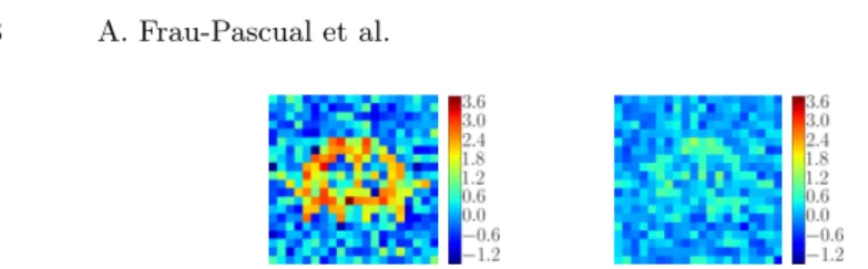
Fig. 3. BRL and PRL ground truth for a noise variance vb“ 7.

4.2 Perfusion response estimation step M2

From the residuals of the first step rM1_{, we estimate the perfusion component.} The remaining signal is, according to (7), @j “ 1 : J ,

yM2 j “ r M1 j “ M ÿ m“1 cm_j W Xmg ` αjw ` bj (10)

In this step, we introduce a prior on g, to account for the already described physiological relationship g “ Ωh:

g|phM1

„ N pΩphM1_{, v}

gΣgq, with Σg“ IF . (11)

The significance of the 2-step approach is to first preprocess the data to subtract the hemodynamic component within the ASL signal, as well as the drift effect, and to focus in a second step on the analysis of the smaller perfusion effect. In [4], differencing methods were used to subtract components with no interest in the perfusion analysis and directly analyse the perfusion effect in the time series. In contrast to these methods, we expect to disentangle perfusion from BOLD components by identifying all the components contained in the signal, and to recover them more accurately.

5 Simulation results

The generative model for ASL time series in section 3 has been used to gen-erate artificial ASL data. A low SNR has been considered, with T R “ 1 s, mean ISI “ 5.03 s, duration 25 s, N “ 325 scans and two experimental con-ditions (M “ 2) represented with 20 ˆ 20-voxel binary activation label maps corresponding to BRL and PRL maps shown in Fig. 3. For both conditions: pamj |qj“ 1q „ N p2.2, 0.3q and pcmj |qj“ 1q „ N p0.48, 0.1q. Parameters were

cho-sen to simulate a typical low SNR ASL scenario, in which the perfusion compo-nent is much lower than the hemodynamics compocompo-nent. A drift `j „ N p0, 10I4q

and noise variance vb“ 7 were considered. BRF and PRF shapes were simulated

with the physiological model, using the physiological parameters used in [8]. In a low SNR context, the PRF estimate retrieved by the former approach developed in [6, 7] is not physilogically relevant as shown in Fig. 4[(c), Top]. In the case of a physiologically informed Bayesian approach, considering a single-step solution as in Fig. 4[Middle], the perfusion component estimation is worse

(10)

∆

BOLD

∆

p

erfusion

time (sec.) time (sec.)

∆ BOLD signal ∆ p erfusion signal

Fig. 4. Results on artificial data. Top row: non-physiological version. Middle row: physiological 1-step version. Bottom row: physiological 2-steps version. (a,d): esti-mated BRL and PRL effect size maps respectively. The ground-truth maps for the BRL and PRL are depicted in Fig.3. (b,c): BRF and PRF estimates, respectively, with their ground truth.

than for the approach described in [6, 7] and the BRF estimation is also degraded owing to the influence of the noisier perfusion component during the sampling. In contrast, the 2-steps method proposed here delivers a PRF estimate very close to the simulated ground truth (see Fig. 4[(c), Bottom] with a BRF which is well estimated too.

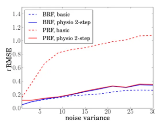
In Fig. 5, the robustness of both approaches with respect to the noise variance is studied, in terms of BRF and PRF recovery. The relative root-mean-square-error (rRMSE) is computed for the PRF and BRF estimates, i.e. rRMSEφ “

}pφ ´ φptrueq}{}φptrueq} where φ P th, gu. We observed that maintaining a good performance in the BRF estimation, we achieved a much better recovery of the PRF for noise variances larger than vb “ 1. Therefore, with the introduction

of the physiological link between BRF and PRF, we have improved the PRF estimation.

6 Real data results

Real ASL data were recorded during an experiment designed to map auditory and visual brain functions, which consisted of N “ 291 scans lasting T R “ 3 s,

(11)

Fig. 5. Relative RMSE for the BRF and PRF and the two JDE versions, wrt noise variance vbranging from 0.5 to 30.

with T E “ 18 ms, FoV 192 mm, each yielding a 3-D volume composed of 64 ˆ 64 ˆ 22 voxels (resolution of 3 ˆ 3 ˆ 3.5 mm3_{). The tagging scheme used}

was PICORE Q2T, with T I1 “ 700 ms, T I2 “ 1700 ms. The paradigm was

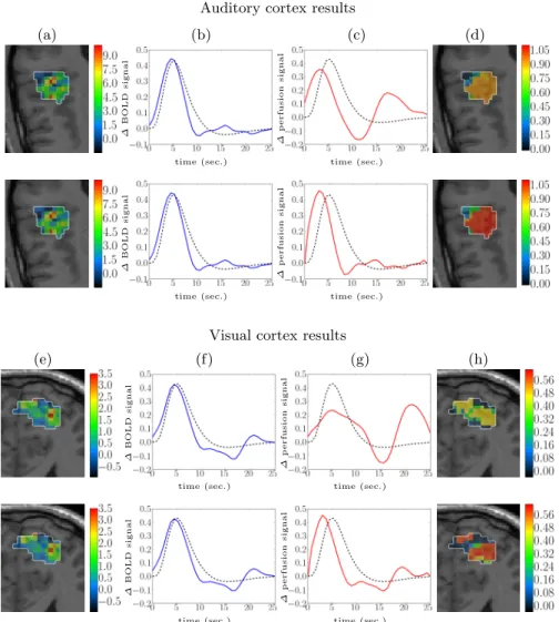
a fast event-related design (mean ISI “ 5.1 s) comprising sixty auditory and visual stimuli. Two regions of interest in the right temporal lobe, for the auditory cortex, and left occipital lobe, for the visual cortex, were defined manually.

Fig. 6(b-c) depicts the response estimates superimposed to the canonical shape which is in accordance with the BRF estimates for both methods. Indeed, we consider here an auditory region where the canonical version has been fit-ted. Accordingly, the BRL maps (Fig. 6(a)) also look alike for both methods. However, PRF estimates significantly differ and the effect of the physiologically-inspired regularization yields a more plausible PRF shape for the 2-steps ap-proach compared with the non-physiological JDE version. Results on PRL maps (Fig. 6(d)) confirm the improved sensitivity of detection for the proposed ap-proach. In the same way, in the visual cortex, Fig. 6(f-g) shows the BRF and PRF estimates, giving a more plausible PRF shape for the 2-steps approach, too. For the detection results (Fig. 6(h)), the 2-steps approach seems also to provide a much better sensitivity of detection.

7 Discussion and conclusion

Starting from non-linear systems of differential equations induced by physio-logical models of the neuro-vascular coupling, we derived a tractable linear op-erator linking the perfusion and BOLD responses. This opop-erator showed good approximation performance and demonstrated its ability to capture both real-istic perfusion and BOLD components. In addition, this derived linear operator was easily incorporated in a JDE framework at no additional cost and with a significant improvement in PRF estimation, especially in critical low SNR sit-uations. As shown on simulated data, the PRF estimation has been improved while maintaining accurate BRF estimation. Real data results seem to confirm

(12)

2. Ogawa, S., Tank, D., Menon, R., Ellermann, J., Kim, S.G., Merkle, H., Ugurbil, K.: Intrinsic signal changes accompanying sensory stimulation: functional brain mapping with magnetic resonance imaging. Proc. Natl. Acad. Sci. USA 89 (1992) 5951–5955

3. Hernandez-Garcia, L., Jahanian, H., Rowe, D.B.: Quantitative analysis of arterial spin labeling fmri data using a general linear model. Magnetic resonance imaging 28(7) (2010) 919–927

4. Mumford, J.A., Hernandez-Garcia, L., Lee, G.R., Nichols, T.E.: Estimation effi-ciency and statistical power in arterial spin labeling fmri. Neuroimage 33(1) (2006) 103–114

5. Vincent, T., Risser, L., Ciuciu, P.: Spatially adaptive mixture modeling for analysis of within-subject fMRI time series. IEEE Trans. Med. Imag. 29(4) (April 2010) 1059–1074

6. Vincent, T., Warnking, J., Villien, M., Krainik, A., Ciuciu, P., Forbes, F.: Bayesian Joint Detection-Estimation of cerebral vasoreactivity from ASL fMRI data. In: 16th Proc. MICCAI, LNCS Springer Verlag. Volume 2., Nagoya, Japan (September 2013) 616–623

7. Vincent, T., Forbes, F., Ciuciu, P.: Bayesian BOLD and perfusion source separation and deconvolution from functional ASL imaging. In: 38th Proc. IEEE ICASSP, Vancouver, Canada (May 2013) 1003–1007

8. Friston, K.J., Mechelli, A., Turner, R., Price, C.J.: Nonlinear responses in fMRI: the balloon model, Volterra kernels, and other hemodynamics. Neuroimage 12 (June 2000) 466–477

9. Buxton, R.B., Uluda˘g, K., Dubowitz, D.J., Liu, T.T.: Modeling the hemodynamic response to brain activation. Neuroimage 23 (2004) S220–S233

10. Buxton, R.B., Wong, E.C., R., F.L.: Dynamics of blood flow and oxygenation changes during brain activation: the balloon model. Magn. Reson. Med. 39 (June 1998) 855–864

11. Khalidov, I., Fadili, J., Lazeyras, F., Van De Ville, D., Unser, M.: Activelets: Wavelets for sparse representation of hemodynamic responses. Signal Processing 91(12) (December 2011) 2810–2821

12. Makni, S., Ciuciu, P., Idier, J., Poline, J.B.: Bayesian joint detection-estimation of brain activity using MCMC with a Gamma-Gaussian mixture prior model. In: 31th Proc. IEEE ICASSP. Volume V., Toulouse, France (May 2006) 1093–1096

(13)

Auditory cortex results (a) (b) (c) (d) ∆ BOLD signal ∆ p erfusion signal

Visual cortex results

(e) (f) (g) (h) ∆ BOLD signal ∆ p erfusion signal

Fig. 6. Comparison of the two JDE versions on real data in the auditory and visual cortex. (top row in auditory and visual cortex results): non-physiological version. (bottom row in auditory and visual cortex results): physiological 2-steps version. (a,e) and (d,h): estimated BRL and PRL effect size maps, respectively. (b,f ) and (c,g): BRF and PRF estimates, respectively. The canonical BRF is depicted as a black dashed line, while PRF and BRF estimated are depicted in solid red and blue lines, respectively.