HAL Id: hal-00850824
https://hal.archives-ouvertes.fr/hal-00850824v2
Preprint submitted on 10 Feb 2014
HAL is a multi-disciplinary open access
archive for the deposit and dissemination of
sci-entific research documents, whether they are
pub-lished or not. The documents may come from
teaching and research institutions in France or
abroad, or from public or private research centers.
L’archive ouverte pluridisciplinaire HAL, est
destinée au dépôt et à la diffusion de documents
scientifiques de niveau recherche, publiés ou non,
émanant des établissements d’enseignement et de
recherche français ou étrangers, des laboratoires
publics ou privés.
High-Multiplicity Scheduling on One Machine with
Forbidden Start and Completion Times
Michaël Gabay, Christophe Rapine, Nadia Brauner
To cite this version:
Michaël Gabay, Christophe Rapine, Nadia Brauner. High-Multiplicity Scheduling on One Machine
with Forbidden Start and Completion Times. 2013. �hal-00850824v2�
(will be inserted by the editor)
High-Multiplicity Scheduling on One Machine with Forbidden
Start and Completion Times
Micha¨el Gabay · Christophe Rapine · Nadia Brauner
Received: date / Accepted: date
Abstract We are interested in a single machine schedul-ing problem where jobs can neither start nor end on some specified instants, and the aim is to minimize the makespan. This problem may model the situation where an additional resource, subject to unavailabil-ity constraints, is required to start and to finish a job. We consider in this paper the High-Multiplicity version of the problem, when the input is given using a com-pact encoding. We present a polynomial time algorithm for large diversity instances (when the number of dif-ferent processing times is greater than the number of forbidden instants). We also show that this problem is Fixed-Parameter Tractable when the number of forbid-den instants is fixed, regardless of jobs characteristics. Keywords Scheduling · High-Multiplicity · Availabil-ity Constraints · Parametrized ComplexAvailabil-ity
1 Introduction
We consider a scheduling problem on one machine where a set of instants is given, such that no job is allowed to start or to complete at any of these instants. We refer to such an instant as a forbidden start & end in-stant (Fse). Forbidden instants may arise when jobs
M. Gabay
Grenoble-INP / UJF-Grenoble 1 / CNRS, G-SCOP UMR5272 Grenoble, F-38031, France
E-mail: [email protected] C. Rapine
Universit´e de Lorraine, Laboratoire LGIPM, Ile du Saulcy, Metz, F-57045, France
E-mail: [email protected] N. Brauner
Grenoble-INP / UJF-Grenoble 1 / CNRS, G-SCOP UMR5272 Grenoble, F-38031, France
E-mail: [email protected]
need some additional resources at launch and comple-tion and these resources are not continuously available. This may be the case if the additional resources are shared with other activities. For example, consider the situation where the jobs are processed by an automated device during a specified amount of time, but a qualified operator is required on setup and completion. While the device is continuously available, the operators have days off and other planed activities. On these days, jobs can be performed by the device, but none can start or com-plete. We encountered this problem in chemical indus-try through a collaboration with the Institut Fran¸cais du P´etrole. In their problem, jobs were chemical exper-iments whose durations typically last between 3 days and 3 weeks. A chemist is required on jobs start and completion to control the process. Each intervention of the chemist can be performed within an hour, but re-quires of course a chemist to be available and present in the laboratory. For more details on this application, we refer the reader to Brauner et al (2009) and Rapine et al (2012).
Notice that, contrary to a classical unavailability constraint, the machine can be processing a job dur-ing an Fse instant, as long as it started its execution before the forbidden instant and will complete after it. We restrict to integer values for the data and to sched-ules where all the jobs start and complete at integer instants. The objective is to minimize the makespan Cmax. Using Graham notations, the problem is denoted
by 1|Fse|Cmax. As an example, consider the instance
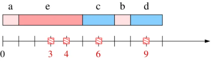
where instants 3, 4, 6 and 9 are Fse instants and 5 jobs have to be scheduled: a and b of duration 1, c and d of duration 2 and e of duration 4. On Figure 1 and 2, forbidden instants are represented on the time axis by dashed rectangles. The sequence of jobs (a, e, c, b, d) leads to an idle-free schedule represented Figure 1 ; the
2 M. Gabay, C. Rapine, N. Brauner
makespan of this schedule is 10. On Figure 2, we have represented the scheduling of the jobs according to the LPT sequence (e, d, c, b, a), that is in non-increasing or-der of the processing times. In oror-der to respect the for-bidden instants, two idle slots are used in the schedule. One can check that the SPT sequence (a, b, c, d, e) leads to a worse schedule, of makepsan 14.
e
c
b
d
0 3 4 6 9
a
Fig. 1: Sequence (a, e, c, b, d). The schedule is idle-free and completes at time 10.
e
d
c
b
a
4
3 6 9
0
Fig. 2: Sequence (e, d, c, b, a). The schedule completes at time 12.
The problem of scheduling jobs on a single machine where a set of time slots is forbidden for starting or com-pleting the jobs has been first investigated by Billaut and Sourd (2009). They considered the case where some time slots are forbidden for starting the jobs, namely the Fs instants (for forbidden start). They proved that minimizing the makespan is polynomially solvable if the number of forbidden start times is fixed, and N P-hard in the strong sense if this number is part of the input. Their algorithm runs in time O(n2k2+2k−1), where k
denotes the number of Fs instants and n is the num-ber of jobs. They also established that if there are at least 2k(k + 1) distinct processing times of the jobs in the instance, then an idle-free schedule exists. Rapine and Brauner (2013) generalized this results: they es-tablished that having k + 1 distinct processing times is a sufficient condition to ensure the existence of an idle-free schedule in presence of k Fse instants. Such an optimal schedule can be found in O(k3
n). As a con-sequence, the overall complexity to solve the problem for a fixed number of forbidden instants is reduced to O(nk). Chen et al (2013) Consider the same problem
with a different objective function, namely the total completion time.
High-multiplicity encoding
The number of types of jobs, that is the number of dif-ferent job durations, play a central role in the above mentioned results. Hence, it is natural to consider a compact encoding where similar jobs are grouped to-gether. The problem then falls in the field of High-Multiplicity Scheduling introduced by Hochbaum and Shamir (1991). Compared to a traditional encoding, where each job is described, in a high-multiplicity (HM) encoding, each type is described only once, along with its multiplicity (the number of jobs of this type). Thus the size of a HM encoding depends linearly on the num-ber of types but only logarithmically on the numnum-ber of jobs. As a consequence, a polynomial time algorithm under the standard encoding may become exponential under a HM encoding of the input, which is the case of the previously mentioned algorithms. HM scheduling and more generally HM combinatorial optimization has become an active domain in recent years, see (Brauner et al 2005; Clifford and Posner 2001; Filippi and Agnetis 2005; Filippi and Romanin-Jacur 2009).
The goal of this paper is to explore the complexity of problem 1|Fse|Cmaxunder a high-multiplicity encoding
of the input. We show that essentially the main results established in the literature under a standard encoding remain valid under a HM encoding. Specifically, we pro-pose in Section 2 a polynomial time algorithm for large diversity instances, that is when the number of types is greater than the number of Fse instants. In Section 3, we also prove that the general problem remains poly-nomial when k is fixed. We first introduce the following notations which will be used in the remaining of the paper.
Notations
Throughout the paper k denotes the number of Fse instants in the instance. Let γi be the i-th Fse instant
with γ1 < γ2... < γk. We denote by F = {γ1, . . . , γk}
the set of the Fse instants. Two jobs are of different types if and only if their processing times are different. The number of types of jobs in the instance is denoted by s. Without loss of generality, we index the types by decreasing order of the processing times of their jobs. The set of jobs to schedule is represented in a HM en-coding by a multiplicity vector (m1, . . . , ms), together
with a processing times vector (p1, . . . , ps), where mi
and pi are respectively the number of jobs of the ith
type and its corresponding processing time. The num-ber of jobs is n =Psi=1mi. The instance of Figures 1 is
thus represented by the processing times vector (4, 2, 1) and the multiplicity vector (1, 2, 2). A job is said to
crossan Fse instant γi if it starts its processing before
γi and ends after γi. For instance in Figure 1, the job
e crosses the first two Fse instants.
We denote by |x| the size of the input under a HM encoding. We have |x| = O(s log n + s log p1+ k log γk).
Hence |x| can be in O(s log n) while the algorithm pro-posed in Rapine and Brauner (2013) runs in time O(k3
n), which can be exponential with respect to |x|.
In HM scheduling, it may not be obvious to deter-mine whether or not schedules can be described with a compact encoding, i.e. polynomial in |x|. For the problem we consider, it is readily that the schedule of the jobs between two forbidden instants is meaningless (provided unnecessary idle-times are not inserted). As a consequence any schedule has a polynomial encod-ing as a sequence of k vectors (m1
i, . . . , msi) and k pairs
(ji, si), where mji is the number of jobs of type j
sched-uled between γi−1and γi ; ji is the job crossing γi and
si its starting time.
An instance is denoted by x = (N, F) where N is the set of jobs. We say that an instance is of large diversity if s > k, that is, if the number of distinct types is greater than the number of forbidden instants. In the reverse situation, we say that the instance is of small diversity.
2 A polynomial time algorithm for large diversity instances
In this section, we design a polynomial algorithm for large diversity instances. Rapine and Brauner (2013) proved that, in such cases, there exists and idle-free schedule:
Theorem 1 (Rapine and Brauner (2013)) If s > k and 0, p(N ) /∈ F, then there exists a feasible schedule without idle time.
They also presented an algorithm, called L-partition, finding an idle-free schedule for large diversity instances in O(k3
n) time, where n = Psi=1mi is the number of
jobs. Although linear in the number of jobs, this algo-rithm is not polynomial with a high-multiplicity encod-ing, except if the multiplicity of each type is bounded by a constant. In particular if only one job is associated with each type, the L-partition algorithm runs in time O(k3
s). We use this fact in our approach.
To design a polynomial time algorithm under a HM encoding, we need to schedule more than one job at a time. We also need an efficient way to decompose the problem. Consider a large diversity instance x = (N, F). Notice that Theorem 1 ensures that an optimal schedule is idle free, assuming that neither instant 0 nor instant p(N ) is forbidden. A schedule is said partial if
only a subset of the jobs is scheduled. We introduce the following definition:
Definition 1 A partial schedule π is an optimal prefix if there exists an optimal schedule of the form πσ.
Consider a partial schedule π completing at time t. Looking at the definition, deciding if π is an optimal prefix may request to compute an optimal schedule for the whole instance. However, by Theorem 1, a sufficient condition for π to be an optimal prefix is that π is idle-free, and that the remaining instance x′ = (N′, F′ =
F ∩ [t, +∞[) is a large diversity instance. Indeed, it guarantees the existence of an idle-free schedule σ for the remaining jobs to schedule after time t.
If we are able to find an optimal prefix π, the prob-lem is reduced to finding an optimal schedule starting at time t on the remaining set N′ of jobs. We can then
look again for an optimal prefix π′ on the remaining
large diversity instance x′. However, for this
decompo-sition to be efficient, we need to bound the number of times an optimal prefix is searched for. We say that a prefix π is efficient if it is optimal and crosses at least one forbidden instant. It is then immediate that at most k efficient prefixes need to be computed to build an op-timal schedule.
Algorithm 1 Optimal Prefix Algorithm
Require: a large diversity instance (N ,F ) with types in-dexed by decreasing order of processing times pj.
Ensure: an optimal prefix π set mi= mi− 1 for i = 1 to k + 1
i = 1 ; t = 0 ; π = ∅ ;
whilei ≤ s and t + mipi< γ1do
{Append the mijobs of type i to π}
π = π(i, mi) ; t = t + mipi; i = i + 1 ;
end while if i > s then
return π {Only k + 1 jobs remain to schedule} end if
{Append as many jobs of type i as possible, before γ1}
α = ⌈(γ1− t)/pi⌉ − 1 ; π = π(i, α) ; t = t + αpi;
{Extend π to complete after time γ1}
for l = 1 to k + 1 such that t + pl≥ γ1 do
if t + pl∈ F then/
return π(l, 1) end if
end for
for l = 2 to k + 1 such that t + pl< γ1 do
if t + pl+ p1∈ F then/
return π(l, 1)(1, 1) end if
end for
Algorithm 1 finds an (efficient) optimal prefix. The main idea of the algorithm is to put aside initially one job of each of the k + 1 largest types. Let B be this set of jobs. This reserve B is used to ensure that the
4 M. Gabay, C. Rapine, N. Brauner
remaining instance is of large diversity. Notice that we can afford to use one of these jobs each time a forbid-den instant is crossed. We call additional jobs the set A = N \B. The algorithm iteratively schedules all the additional jobs of type 1, then all the additional jobs of type 2, and so on. Recall that types are indexed in de-creasing order of the processing times, thus we simply follow a LPT sequence for the additional jobs. We keep scheduling additional jobs as long as they fit before the first forbidden instant γ1. When this process halts on
some index i, either only the jobs from the set B remain to schedule, or there is not enough room left before γ1
to schedule all the additional jobs of the ith type. In the latter case, the algorithm schedules as much jobs of type i as possible before γ1. Then, it tries to cross the
forbidden instant γ1. In order to keep a large diversity
instance, we ensure that each job of B scheduled allows to cross at least one forbidden instant. This way the algorithm outputs an efficient prefix. In the other case, all additional jobs have been scheduled and the partial schedule returned is optimal but not efficient, since the first Fse instant is not crossed. However, we are in the situation where the remaining large diversity instance contains only one job per type, and we have exactly k + 1 types. We can use the L-partition algorithm to solve it efficiently, in time O(k4). The correctness of the
algorithm is summarized in the following lemma: Lemma 1 Given a large diversity instance x = (N, F), Algorithm 1 delivers an optimal prefix π. In addition, if x′ = (N′, F′) is the remaining instance to schedule,
thenx′ is a large diversity instance and:
1. either|F′| < |F|, that is π is an efficient prefix,
2. or |N′| = |F| + 1 and all the remaining jobs have
distinct processing times.
Proof Let (N′, F′) be the instance remaining to
sched-ule at the end of Algorithm 1. Recall that B denotes a set with exactly one job of the k + 1 largest types of N and A = N \B is the set of the additional jobs. If only the set B remains to schedule at the end of the algorithm, then we are clearly in the second case of our claim: |N′| = k + 1. Otherwise the algorithm
has stopped the first loop on a type i such that all the additional jobs cannot be scheduled before γ1. At this
point, there is at least one unscheduled job of type i remaining in A, and possibly another in B, if i ≤ k + 1. Let t < γ1be the current completion time of the
sched-ule, and consider the partition B = S ∪ L defined by L = {j ∈ B | t + pj ≥ γ1} and S = B\L. Notice that
L is not empty as t + pi ≥ γ1 ; in particular a job of
type 1 belongs to L. By construction the prefix algo-rithm tries to extend π in order to complete after the first forbidden instant γ1. We have to prove that it will
always succeed, and that (N′, F′) is a large diversity
instance. We denote by s′ the number of distinct types
of jobs in the remaining instance x′ and by k′ = |F′|
the number of Fse instants appearing after time t. In the following, we show that if π completes after the lth forbidden instant, at most l jobs of B have been scheduled in π. As a consequence, s′≥ |B| − l > k − l ≥
k′ and (N′, F′) is a large diversity instance. Consider
the last two loops of the algorithm. If one job of L can be scheduled, the property clearly holds as π completes after time γ1. If there is no such job, then for all jobs
j of L, t + pj is a forbidden instant while any job of
S can be scheduled before time γ1. Therefore a simple
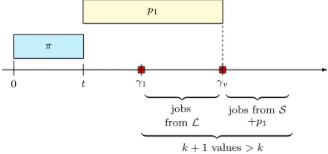
counting argument, illustrated Figure 3, ensures that there exists a job s ∈ S which can be scheduled at time t immediately followed by a job of type 1. If t + ps+p1≥ γ2, i.e. π completes after time γ2, we are done.
Otherwise, we have t + p1< γ2. In this case k′= k − 1,
while we apparently use 2 jobs of B. However, instant t + p1 is forbidden ; in fact we have t + p1 = γ1 and
as a consequence i = 1. As we noticed, there is at least one unscheduled job of type i in A. Since i = 1, we can use an additional job of type 1, instead of using a job of type 1 from B. We have s′ ≥ s − 1 which completes
the proof. ⊓⊔ π p1 t γ1 γv 0 ✲ | {z } | {z } | {z } jobs from L jobs from S +p1 k + 1 values > k
Fig. 3: Counting argument: the first Fse instants can be crossed using one or two jobs from B.
In order to deliver an optimal schedule, we itera-tively call the prefix algorithm on the remaining in-stance as long as we obtain an efficient prefix. Other-wise, we are in the second case of Lemma 1, which cor-responds to the basis of the recursion: we simply solve instance x′ = (N′, F′) using the L-partition algorithm.
Since N′ contains at most (k + 1) jobs, the running
time of the L-partition algorithm on this instance is in O(k4). We have the following theorem:
Theorem 2 Problem 1|Fse|Cmax is polynomial under
HM encoding for large diversity instances, and can be solved in timeO(sk + k4)
Proof From the above discussion, we only need to es-tablish the time complexity of the algorithm, its cor-rectness being a direct consequence of Lemma 1. We use
the classic convention that basic operations on integers (addition, division. . . ) are performed in constant time. Then the time complexity of Algorithm 1 is in O(k +s), which is in O(s) for large diversity instances. To solve Problem 1|Fse|Cmax, we call Algorithm 1 on the set of
unscheduled jobs as long as there is still some forbid-den instants in the future or that this set is not reduced to B. Thus we have at most k calls to Algorithm 1, pos-sibly followed by a call to L-partition algorithm on an instance containing at most k + 1 jobs. Therefore the overall complexity is in O(sk + k4
). ⊓⊔ If 0 or p(N ) are in F, then the same transformation as in Rapine and Brauner (2013) allows to obtain an optimal schedule. Note that, even under a traditional encoding of the instance, the optimal prefix algorithm has a better time complexity than the L-partition algo-rithm which runs in time O(k3
n).
3 A polynomial time algorithm for a fixed number of Fse
In this section we establish that the problem 1|Fse|Cmax
can be solved in polynomial time under a HM encoding of the instances if the number of forbidden instants is fixed, that is, if k is not part of the input. This result ex-tends a theorem from Rapine and Brauner (2013) which establishes that 1|k − Fse|Cmax is polynomial under a
standard encoding, that is, its complexity is polynomi-ally bounded in n, the number of jobs (but not in s, the number of types). The rest of the section is devoted to proving the following theorem:
Theorem 3 The problem 1|Fse|Cmax is Fixed
Param-eter Tractable for paramParam-eter k, even under high-multi plicity encoding of the input.
Notice that if the instance is of large diversity, the optimal prefix algorithm (Algorithm 1, Section 2) can deliver an idle-free (and thus optimal) schedule in time O(s) for any fixed number k of forbidden instants. Hence we can focus on the case of small diversity instances. Our idea is to formulate the problem on small diver-sity instances as an integer linear program (ILP) with a fixed number of variables and constraints. Such an ILP can be solved in polynomial time, due to the fol-lowing result from Eisenbrand (2003):
Theorem 4 (Eisenbrand (2003)) An integer pro-gram of binary encoding length l in fixed dimension, which is defined by a fixed number of constraints, can be solved with O(l) arithmetic operations on rational numbers of binary encoding length O(l).
For small diversity instances, we have by definition s ≤ k. Thus, if the number of variables and the number of constraints in our ILP formulation are bounded by a polynomial in k, Theorem 4 implies that 1|Fse|Cmax
is FPT with respect to parameter k. Clearly, to obtain such a formulation, we can not afford to introduce one decision variable (such as the completion time) or one constraint (such as avoiding to complete on a forbidden instant) for each job. Instead, as already discussed in the HM encoding of a solution, see Section 1, we rep-resent a solution by the number of jobs of each type scheduled between two consecutive forbidden instants. However, this representation of the solution is suitable only for idle-free schedules, since otherwise one has also to give the starting time of each block of jobs. To for-mulate the problem as an ILP, we take advantage of the fact that any large diversity instance admits an idle-free schedule, see Theorem 1. More precisely, we transform a small diversity instance I into a large diversity in-stance I′ by adding dummy jobs as follows. Given an
instance I composed of s types, I′ is constituted of the
following types:
– Real jobs. They are the jobs of I. We denote by pi
and mi the processing time and the multiplicity of
the type i, for i = 1, . . . , s.
– Optional jobs. We add k + 1 types to ensure that there exists an idle free schedule. For i = s + 1 to s + k + 1, type i has a processing time pi = i − s
and its multiplicity is unbounded.
The number of jobs of the instance I′ is unbounded
due to the optional jobs. However, as their name sug-gests, a schedule π′ for I′ does not need to schedule
all the optional jobs. More precisely, we do not request to schedule any optional job once all the real jobs have been processed and all the forbidden instants have been crossed. We denote by eCmax(π′) the completion time of
the last real job of π′. We have the following property:
Property 1 There exists a schedule π for the instance I with makespan Cmax(π) if and only if there exists
an idle-free schedule π′ for the instance I′ such that
e
Cmax(π′) = Cmax(π).
Proof Given a schedule π′ for I′, we immediately
ob-tain a valid schedule for the instance I by replacing the optional jobs by idle times with the same duration. The jobs of I are processed at the same dates as in π′, and
thus clearly the makespan is equal to eCmax(π′).
Con-versely, consider a schedule π for instance I. We have to prove that for each idle period [u, v] occurring in π, we can sequence optional jobs to obtain an idle-free schedule. Since π is feasible, u and v cannot be forbid-den instants. Thus, if the idle period is short, that is
6 M. Gabay, C. Rapine, N. Brauner
v − u ≤ k + 1, we can simply schedule an optional job of duration v − u. Otherwise, we have v ≥ u + (k + 2). Since there are k forbidden instants in the instance, at least one instant in the time interval [u + 1, u + k + 1] is not forbidden. Let t be the last forbidden instant be-fore u + 1 + k which is not forbidden. In π′, at time u,
we schedule an optional job of duration t − u ≤ k + 1. By immediate induction we can fill the remaining idle period [t, v] with optional jobs. ⊓⊔ Based on Property 1, we show that we can use an ILP with a fixed number of variables and constraints to find an idle-free schedule π′ minimizing the completion
time of the last real job. We denote by s′ ≥ k + 1 the
number of types (real and optional) in the instance I′.
By construction I′ is of large diversity, that is s′ > k,
and thus we know that an idle-free schedule π′ exists.
To bound the completion time of the last real job, we use the property (see Rapine and Brauner (2013)) that any list scheduling algorithm produces a schedule with makespan at most Q = 2k +Psi=1mipi. Thus Q is an
upper bound on the completion time of the last real job in an optimal schedule for I′. As a consequence we
can assume without loss of generality that γk≤ Q − 2,
since the last Fse instants can be discarded till this in-equality holds. We also add a very large optional job of processing time ps+k+2= γk+1. This job allows to cross
all the remaining Fse instants if the schedule finishes before the last one. Finally, for the ease of presentation, we introduce the notation γk+1= Q + ps+k+2+ 1.
As already discussed, we can represent an idle-free schedule by giving the number of jobs of each type sequenced between any two consecutive forbidden in-stants (or alternatively by giving the cumulative num-ber of jobs completed before any forbidden instant) and the jobs crossing forbidden instants. We have the fol-lowing decision variables:
mij number of jobs of type i completed by time
γj for i = 1, . . . , s′ and j = 1, . . . , k + 1.
Sjf = 1 if a job crosses exactly the instants γj
till γf −1 (included), for j = 1, . . . , k and
f = j + 1, . . . , k + 1. = 0 otherwise
xij = 1 if a job of type i crosses the instant γjand
this job does not cross the previous Fse instant, for i = 1, . . . , s′ and j = 1, . . . , k.
= 0 otherwise
yj = 1 if all real jobs have been completed by
time γj, for j = 1, . . . , k.
= 0 otherwise e
Cmax completion time of the last real job.
The variables mij are non-negative integers, Sjf,
xij, yjare boolean variables and eCmaxis a non-negative
real. We also define variable Wj as the total work
com-pleted by time γj for j = 1, . . . , k + 1. Notice that we
do not distinguish real from optional jobs in the def-inition of Wj, that is Wj is simply a short-hand for
Ps′
i=1pimij. Also notice that Wj does not take into
ac-count the processing time of a job started but not yet completed, that is a job that would cross the forbidden instant γj. Hence a job crossing the forbidden instants
γj but not γj−1 must start at time Wj in an idle-free
schedule.
The following linear formulation finds an idle-free schedule minimizing the completion time of the last real job for the instance I′:
Minimize eCmax, subject to the constraints:
– All Fse are crossed, which is equivalent to require that variables Sjf define a 1 − (k + 1) path:
k+1 X f =2 S1f = 1 (1) k X j=1 Sj,k+1= 1 (2) f −1 X j=1 Sjf = k+1 X l=f +1 Sf l ∀f = 2, . . . , k (3)
– A job crosses γj as its first Fse instant if and only
if Sjf = 1 for some index f > j: s′ X i=1 xij = k+1 X f =j+1 Sjf ∀j = 1, . . . , k (4)
– For each type, the variable mij is increasing with j.
In addition, if a job of type i crosses γj, then the
number of jobs of type i completed should increase by at least one after the next forbidden instant fol-lowing the completion of the job.
mi,j+1 ≥ mij ∀i = 1, . . . , s′ ∀j = 1, . . . , k (5) mif ≥ mij+ xij+ Sjf− 1 ∀i = 1, . . . , s′ 1 ≤ j < f ≤ k + 1 (6)
– Schedule all the real jobs:
mi,k+1= mi ∀i = 1, . . . , s (7)
– Set yj = 0 if all the real jobs are not completed
before the instant γj: s X i=1 mij ≥ yj s X i=1 mi ∀j = 1, . . . , k (8)
– Definition of the work Wj: Wj= s′ X i=1 mijpi ∀j = 1, . . . , k + 1 (9)
– All the work Wj must be completed by time γj:
Wj≤ γj− 1 ∀j = 1, . . . , k + 1 (10)
– The amount of work completed can not increase be-tween instants γj and γf −1 if a job crosses these
instants, that is Sjf = 1:
Wf −1≤ Wj+ Q(1 − Sjf) ∀1 ≤ j < f ≤ k + 1
(11) – If Sjf = 1 and a job of type i crosses γj, then this
job should complete in the time interval [γf −1 +
1, γf − 1]: Wj+ s′ X i=1 pixij ≥ k+1 X f =j+1 (γf −1+ 1)Sjf ∀j = 1, . . . , k (12) Wj+ s′ X i=1 pixij ≤ γj− 1 + k+1 X f =j+1 (γf− γj)Sjf ∀j = 1, . . . , k (13) – The makespan should be equal to the first Wj such
that yj = 1:
e
Cmax≥ W1 (14)
e
Cmax≥ Wj− yj−1Q ∀j = 2, . . . , k + 1 (15)
Constraints (1)-(2)-(3) are classical flow conserva-tion equaconserva-tions. They impose all the forbidden instants to be crossed in an idle-free schedule. If a job crosses the forbidden instants γjup to γf −1, Constraint (4) ensures
that exactly one variable xij is set to 1 to represent
the type of this job ; Reciprocally if one job crosses γj
and not the preceding forbidden instant, Constraint (4) ensures that exactly one variable Sjf is set to 1, to
represent the set of Fse instants crossed by the job. Constraint (6) forces the number of completed jobs of type i to increase by at least one between forbidden in-stants γj and γf if a job of type i crosses exactly all
the Fse instants from γj to γf −1. Notice that in this
case we have xij = 1 and Sjf = 1, which imposes that
mif > mij. As we know that an optimal schedule
se-quences the last real job before instant γk+1, we can
impose through Constraint (7) that all the real jobs are completed by this time.
Constraint (10) ensures that the completion time of the last job completing before the instant γj does
not coincide with this instant. Constraint (11) prevents from scheduling some jobs between forbidden instants crossed by a same job: if variable Sjf is equal to 1,
then the constraint boils down to Wf −1 ≤ Wj. Due to
Constraint (5), Wlis increasing with the index l. Hence
we have Wj= Wj+1= · · · = Wf −1: The work achieved
by time γf −1is still Wj. On the contrary if Sjf is equal
to zero, the constraint becomes redundant.
Constraints (12) and (13) prevent a job crossing the forbidden instant γj from completing on another
for-bidden instant. If Sjf = 1 for some index f ≤ k and
the crossing job is of type i (xij = 1), the constraints
force γf −1 + 1 ≤ Wj + pi ≤ γf − 1. Notice that if
f = k + 1, Constraint (13) becomes redundant. Finally if Sjf = 0 for all indices f > j, both constraints are
redundant since all the variables xij are zero due to
Constraint (4) already discussed, and the right hand sides are then equal respectively to 0 and γj− 1. Thus
(12) states that Wj is non negative and (13) gives
Con-straint (10).
Finally, consider Constraint (15), and let l be the first index such that yl = 1. We claim that this
con-straint imposes at the optimum that eCmax = Wl.
In-deed, if yj−1= 1 the constraint yields eCmax positivity
and if yj−1 = 0, it boils down to eCmax ≥ Wj. Setting
yj = 1 for all j ≥ l is feasible and dominant. Since
we are minimizing eCmax, the inequality eCmax ≥ Wl is
tight. We claim that Wj is precisely equal to the
com-pletion time of the last real jobs in an optimal solution. Indeed, once this last job has been scheduled, if there are some forbidden instants remaining, they can all be crossed by using the optional job s+k+2. This optional job clearly crosses all the remaining forbidden instants, and in particular the instant γl. This shows that the
value of Wl, and thus of eCmax at the optimum, is equal
to the completion time of the last real job.
This integer program delivers an optimal solution to the instance I′ and, using Property 1, we can convert
it into an optimal solution to the original instance I. Moreover, the number of decision variables of the ILP is in O(k2) and the number of constraints is in O(k3).
Thus, we can apply Theorem 4, which proves Theo-rem 3.
4 Conclusion
In this paper, we have generalized to high-multiplicity the results from Rapine and Brauner (2013): we have shown that large diversity instances can be solved in polynomial time also with a high-multiplicity encoding of the input. We proposed an algorithm solving this problem in O(sk + k4) time, improving the
complex-8 M. Gabay, C. Rapine, N. Brauner
ity of the previous algorithm from Rapine and Brauner (2013) even if the input is not provided using a compact encoding.
We modeled 1|Fse|Cmaxas an integer program and
used the existence of an idle-free schedule for large diversity instances to avoid modeling the completion time for each job. The resulting integer program has a fixed number of constraints and variables. Therefore, by Eisenbrand’s theorem, 1|Fse|Cmax is fixed-parameter
tractable, even under high-multiplicity encoding of the input. Such an approach could be used on other high-multiplicity scheduling problems to classify them.
Further research can investigate small diversity in-stances. Especially, it would be interesting to determine whether or not this problem remains polynomial when s is close to k, in particular if s = k.
Other optimization criteria such as minimizing the mean flow time can be investigated as well. Chen et al (2013) have already studied a similar problem, with one operator non-availability period. Further investigations of these problems would be interesting and likely to have important industrial applications.
References
Billaut JC, Sourd F (2009) Single machine scheduling with forbidden start times. 4OR 7(1):37–50
Brauner N, Crama Y, Grigoriev A, Van De Klundert J (2005) A framework for the complexity of high-multiplicity scheduling problems. Journal of combinatorial optimiza-tion 9(3):313–323
Brauner N, Finke G, Lehoux-Lebacque V, Rapine C, Kellerer H, Potts C, Strusevich V (2009) Operator non-availability periods. 4OR 7(3):239–253
Chen Y, Zhang A, Tan Z (2013) Complexity and approx-imation of single machine scheduling with an operator non-availability period to minimize total completion time. Information Sciences 251:150–163
Clifford JJ, Posner ME (2001) Parallel machine schedul-ing with high multiplicity. Mathematical programmschedul-ing 89(3):359–383
Eisenbrand F (2003) Fast integer programming in fixed dimension. In: Battista G, Zwick U (eds) Algorithms -ESA 2003, Lecture Notes in Computer Science, vol 2832, Springer Berlin Heidelberg, pp 196–207
Filippi C, Agnetis A (2005) An asymptotically exact al-gorithm for the high-multiplicity bin packing problem. Mathematical programming 104(1):21–37
Filippi C, Romanin-Jacur G (2009) Exact and approximate algorithms for high-multiplicity parallel machine schedul-ing. Journal of Scheduling 12(5):529–541
Hochbaum DS, Shamir R (1991) Strongly polynomial algo-rithms for the high multiplicity scheduling problem. Op-erations Research 39(4):648–653
Rapine C, Brauner N (2013) A polynomial time algorithm for makespan minimization on one machine with forbid-den start and completion times. Discrete Optimization 10(4):241–250
Rapine C, Brauner N, Finke G, Lebacque V (2012) Single machine scheduling with small operator-non-availability periods. Journal of Scheduling 15(2):127–139