HAL Id: hal-03152932
https://hal.inria.fr/hal-03152932v2
Submitted on 2 Mar 2021
HAL is a multi-disciplinary open access
archive for the deposit and dissemination of
sci-entific research documents, whether they are
pub-lished or not. The documents may come from
teaching and research institutions in France or
abroad, or from public or private research centers.
L’archive ouverte pluridisciplinaire HAL, est
destinée au dépôt et à la diffusion de documents
scientifiques de niveau recherche, publiés ou non,
émanant des établissements d’enseignement et de
recherche français ou étrangers, des laboratoires
publics ou privés.
Deciding Non-Compressible Blocks in Sparse Direct
Solvers using Incomplete Factorization
Esragul Korkmaz, Mathieu Faverge, Grégoire Pichon, Pierre Ramet
To cite this version:
Esragul Korkmaz, Mathieu Faverge, Grégoire Pichon, Pierre Ramet. Deciding Non-Compressible
Blocks in Sparse Direct Solvers using Incomplete Factorization. [Research Report] RR-9396, Inria
Bordeaux - Sud Ouest. 2021, pp.16. �hal-03152932v2�
0249-6399 ISRN INRIA/RR--9396--FR+ENG
RESEARCH
REPORT
N° 9396
February 2021Non-Compressible Blocks
in Sparse Direct Solvers
using Incomplete
Factorization
RESEARCH CENTRE BORDEAUX – SUD-OUEST
Esragul Korkmaz
* §, Mathieu Faverge
*§, Gr´
egoire Pichon
¶,
Pierre Ramet
§ *Project-Team HIEPACS
Research Report n° 9396 — February 2021 — 16 pages
Abstract: Low-rank compression techniques are very promising for reducing memory footprint and execution time on a large spectrum of linear solvers. Sparse direct supernodal approaches are one these techniques. However, despite providing a very good scalability and reducing the memory footprint, they suffer from an important flops overhead in their unstructured low-rank updates. As a consequence, the execution time is not improved as expected. In this paper, we study a solution to improve low-rank compression techniques in sparse supernodal solvers. The proposed method tackles the overprice of the low-rank updates by identifying the blocks that have poor compression rates. We show that block incomplete LU factorization, thanks to the block fill-in levels, allows to identify most of these non-compressible blocks at low cost. This identification enables to postpone the low-rank compression step to trade small extra memory consumption for a better time to solution. The solution is validated within the PaStiX library with a large set of application matrices. It demonstrates sequential and multi-threaded speedup up to 8.5x, for small memory overhead of less than 1.49x with respect to the original version.
Key-words: Sparse direct solvers, low-rank compression, ILU factorization
*Inria Bordeaux - Sud-Ouest, Talence, France Bordeaux INP, Talence, France
CNRS (Labri UMR 5800), Talence, France §University of Bordeaux, Talence, France ¶Univ Lyon, EnsL, UCBL, CNRS, Inria, LIP
D´
etecter les blocs non compressibles dans les
solveurs directs creux par une factorisation
incompl`
ete
R´esum´e : Les techniques de compression de rang faible sont tr`es promet-teuses au niveau de l’empreinte m´emoire et du temps d’ex´ecution sur un large spectre de solveurs lin´eaires. Les approches supernodales directes creuses font partie de ce spectre. Cependant, malgr´e leur tr`es bonne scalabilit´e et leur em-preinte m´emoire plus faible, elles souffrent d’un surcoˆut calculatoire important dˆu aux mises `a jour non-structur´ees de rang faible impliqu´ees. En cons´equence, le temps d’ex´ecution n’est pas am´elior´e comme pr´evu. Dans cet article, nous ´
etudions une solution pour am´eliorer les techniques de compression de rang faible dans les solveurs supernodaux creuses. La m´ethode propos´ee s’int´erresse `a ces mises `a jour de rang faible plus coˆuteuses en identifiant les blocs avec de faibles taux de compression. Nous montrons que la factorisation LU incompl`ete par blocs, grˆace aux niveaux de remplissage des blocs, permet d’identifier, `a faible coˆut, la plupart de ces blocs non compressibles. Cette identification permet de reporter l’´etape de compression de rang faible pour permettre un meilleur temps de r´esolution en ´echange d’une l´eg`ere sur-consommation m´emoire. La solution est valid´ee dans la biblioth`eque PaStiX avec un large ensemble de matrices is-sues d’applications. Il d´emontre une acc´el´eration s´equentielle et multithread jusqu’`a 8.5x, pour une augmentation de la consommation m´emoire inf´erieure `a 1.49x par rapport `a la version originale.
Mots-cl´es : Solveur direct creux, compression de rang faible, factorisation ILU
1
Introduction
In many engineering and scientific applications, solving a large sparse linear sys-tem of the form Ax = b is a mandatory but very time consuming step. Among the many various approaches to solve these systems, sparse direct solvers [9] are a robust and widely used solution. However, they are known to be both time and memory consuming. Recent studies tackle these issues by experimenting different data-sparse compression schemes trading a controlled precision loss for better memory and computation complexities. These techniques include but are not limited to (Multilevel-)Block Low-Rank format (BLR) [1, 3, 21], H-Matrices [11, 17], H2[13], Hierarchical Off-Diagonal Low-Rank (HODLR) [4, 6] or Hierarchically Semi-Separable (HSS) [10, 25]. These techniques can be clas-sified into two categories. The first one considers the full problem and extracts the sparsity of the matrix from the low-rank representation. The second solu-tion exploits the existing sparsity of the matrix structure and compresses the blocks that compose it independently. This paper focuses on the latter. More specifically, it targets block low-rank methods (BLR).
In this context, as in other linear algebra solvers, one of the most impor-tant operation is the block update. When using regular block sizes, as in dense or sparse multifrontal solvers, the cost of the low-rank update is usually small with respect to the full-rank version. On the other hand, when various block sizes are involved, as in sparse supernodal solvers, the cost of the low-rank update depends on the largest block involved. Therefore, the update opera-tion may become more expensive than the full-rank one. However, supernodal approaches provide more parallelism and have less memory overhead than mul-tifrontal methods. As a consequence, in this paper, we propose to improve supernodal methods by trading a small memory overhead for lower flop count and better time to solution. For that purpose, we implement our solution in the sparse direct solver PaStiX [20, 21], which supports the BLR compression scheme.
The PaStiX solver offers two opposite strategies: favor memory peak re-duction over time to solution (Minimal Memory), or prefer time to solution by delaying the data compression (Just-In-Time). The former suffers from the costly update operations, while the latter avoids it without reducing the mem-ory consumption compared to the full-rank solver. Identifying the potential compressibility of each block is a key problem to benefit from both strategies. In this work, we propose a new technique based on incomplete factorization to define levels of admissibility (compressibility) for the blocks. The algorithm is applied during the preprocessing stage and provides a trade-off between mem-ory and flops. We show that this solution, while targeting the Minimal Memmem-ory strategy, may also improve the Just-In-Time solution.
Section 2 sets the basis of this work by giving background information on the BLR implementation within the PaStiX solver and its limitations, as well as in-troducing the block incomplete LU factorization. Section 3 presents the related work. Section 4 details the new heuristic, which defines the non-compressible blocks to exploit the existing compression strategies in PaStiX. Section 5
anal-4 Korkmaz & Faverge & Pichon & Ramet
yses experiments on a large set of matrices. Finally, Section 6 concludes on the results of this work and its perspectives.
2
Background
This section provides background details on the PaStiX solver and its BLR implementation and recalls the general idea behind incomplete LU factorization.
2.1
Sparse supernodal direct solver using BLR
compres-sion
Sparse direct solvers generally follow four steps: 1) order the unknowns to reduce the fill-in that occurs during factorization; 2) perform a block-wise symbolic factorization to compute the structure of the final factorized matrix; 3) compute the actual numerical factorization based on the structure resulting from step 2; and 4) solve the triangular systems. In the remainder of the paper, we will focus only on the numerical factorization (step 3) and the matrix values initialization. We consider that steps 1 and 2 already exhibit a structure with large enough blocks to take advantage of BLAS Level 3 [8] operations whenever possible. Step 4 is not influenced by the work presented in this paper, and is thus not further discussed.
m
M n
N
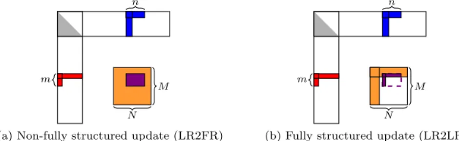
(a) Non-fully structured update (LR2FR)
m
M n
N
(b) Fully structured update (LR2LR)
Figure 1: Representation of the updates, C −= AB, for the Just-In-Time strategy on the left, and Minimal Memory on the right. A appears in red, B in blue, C in orange, and the impact of the contribution AB in purple.
BLR compression scheme has been introduced in the sparse supernodal solver PaStiX in [20, 21]. As already mentioned, the solver implements two strategies to target either lower memory cost (Minimal Memory), or lower time to solution (Just-In-Time). Both strategies differ depending on the update kernels, C = C − AB, that are involved in the numerical factorization. Fig-ure 1 describes both options. On the left, the non-structFig-ured updates (LR2FR) lower the cost of the matrix product AB thanks to the low-rank representation. However, the updated C matrix is stored in full-rank to be able to perform a simple addition of the contribution at a cost of order mn, with m and n the
dimensions of this contribution. On the right, although the low-rank structured update (LR2LR) is more complex, the C matrix is stored in low-rank to save memory. Here, while the contribution (AB) is also computed at a lower cost, the addition step into C requires a more complex low-rank to low-rank update with padding (zeroes are added to match the dimension of C). This update has a complexity of order M N , with M and N the dimensions of the updated matrix C. A more detailed complexity analysis is provided in [21].
The Just-In-Time strategy aims only at reducing the time to solution by exploiting the LR2FR update kernel. Indeed, LR2FR relies on high performance matrix-matrix multiplication kernels with smaller sizes than the ones of the full-rank implementation. On the other hand, the Minimal Memory strategy compresses the matrix at initialization exploiting the graph of the matrix to speedup the compression. Blocks of the factorized matrix which do not hold initial information are null and thus compressed at no cost. Other initial blocks compression can also be accelerated by automatically removing null columns and rows from the graph knowledge. This operation greatly improves the memory peak of the solver as the factorized matrix structure is never fully allocated. However, it forces the numerical factorization to rely on the LR2LR kernel. This kernel in the context of the supernodal method generates a flop overhead due to the padding operation. As a consequence, the factorization time may be highly impacted, unless the matrix is highly compressible. Thus, deciding which blocks to compress and when to do it is an important problem for supernodal solvers to reach good level of performance while benefiting from the lower memory consumption offered by low-rank techniques. Note that in sparse direct solvers, only blocks with sufficiently large sizes are considered to be admissible for low-rank compression. All small blocks are automatically defined as non-admissible due to their lower impact.
To decide which blocks to compress, [12] defined the admissibility condition. More specifically, the study proposes a strong and a weak admissibility condi-tions. The strong admissibility condition relies on the problem geometry and the definition of the diameter of a set of unknowns (diam(σ)), as well as the distance between two sets (dist(σ, τ )). The interaction between two sets of unknowns is then considered admissible if the distance between the sets is sufficiently larger than both of the diameters of the sets (max(diam(σ), diam(τ )) ≤ η dist(σ, τ )). The least restrictive strong admissibility criterion considers that blocks are ad-missible only if their distance is larger than 0. Thus, all blocks except close neighbors are compressible. On the other hand, the weak criterion simply con-siders that all non-diagonal blocks are compressible, which is equivalent to the Minimal Memory strategy. This paper proposes to generalize the distance crite-rion used in the strong admissibility condition by computing algebraic distances of the blocks without any geometry knowledge requirement. The distance com-putation is performed with block-wise ILU factorization.
6 Korkmaz & Faverge & Pichon & Ramet
2.2
Incomplete LU factorization
The incomplete LU (ILU) factorization is an approximated version of the LU factorization, where part of the information is dropped [23]. It has the form A ≈ LU = LU + R. Here, the matrix R carries the negative values of the dropped elements. This method is usually used as a preconditioner for iterative methods [14]. level 1 level 1 4 3 2 1 1 2 3 4 5 5 1 3 2 4 5 level 3
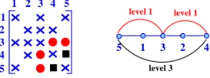
Figure 2: An adjacency matrix (on the left) and its associated graph (on the right). Fill-in entries that may occur during the numerical factorization are represented in red (level 1) and black (level 3).
Numerical or graph constraints are applied to obtain the ILU factorization. For example, the dropping can be based on a threshold [16], or on the fill-in levels [5]. We consider only the latter in this paper. The ILU method with the fill-in levels definition as we use was first suggested in 1981 [24] and then improved by a graph-based definition in [15, 22]. Figure 2 illustrates the idea of the fill-in levels that is strongly related to the ordering of the unknowns. On the left, the matrix non-zeroes pattern is represented, where the blue crosses are the original entries. On the right, the graph associated to this matrix is shown. During the numerical factorization, some entries may become non-zeroes (fill-in). On Figure 2, these entries are represented in red and black, both on the matrix and as new edges on the graph. We can define the fill-in level as the length of the path connecting the two unknowns in the original graph. The path connecting 3 and 5 (and 3 and 4) in red goes only through 1 (resp. 2). Thus, the level of the fill-in between these two unknowns is 1. We can also see that 4 and 5 are connected at a level 3 (the path goes through 1, 3 and 2). As the fill-in level gets higher, the value of the new entry becomes smaller as it represents far interactions in the graph. Therefore, the ILU factorization can be implemented by omitting the values which have higher fill-in levels than a predefined maximum level. Similarly, this procedure can be applied in a block-wise fashion. Thus, the block fill-in level can be considered as an admissibility criterion for low-rank compression.
3
Related work
Many recent studies have tackled the problem of reducing the memory con-sumption of linear solvers with low-rank compression.
In [12], the adaptation of hierarchical matrix techniques issued from the dense community to sparse matrices is studied. Here, by ignoring some struc-tural zeroes, the opportunity for further memory savings is missed. Although
low-rank updates are performed similarly to the Minimal Memory strategy, padding is not used as the zeroes are explicitly stored. This results in more efficient updates at the cost of a larger memory consumption.
Low-rank updates in the context of sparse supernodal solvers have already been studied in [6]. In this work, the authors considered fixed ranks for the blocks which must be known in advance. They demonstrated interesting mem-ory savings, but with a slower factorization than the full-rank version.
The sparse multifrontal BLR solver Mumps [2, 19] implements two similar solutions: CUFS (Compress, Update, Factor, Solve) which is similar to our Min-imal Memory scenario, and FCSU which is closer to the Just-In-Time scenario. However, as it is a multifrontal solver, these strategies are applied with tiled algorithms on the dense matrices of the fronts that appear during the factor-ization. Here, the memory saving is limited as fronts are allocated in full-rank before being compressed.
In [18], the preselection problem is approached from a different angle. The authors exploit performance models of the update kernel to decide whether or not to delay the compression of some of the blocks. This decision is taken at runtime during the numerical factorization and requires to generate correct models of the problem.
4
Deciding the Non-Compressible Blocks
As mentioned in Section 2, the Minimal Memory strategy suffers from the com-plexity overhead of the LR2LR update kernel. We propose to exploit ILU fill-in levels to identify, at low cost, the blocks with large ranks. These blocks will increase the cost of the update step while providing only a small memory reduc-tion. Once identified, it is possible to postpone the compression of these blocks as late as possible to replace the LR2LR kernels by LR2FR. This comes to the cost of a controlled memory overhead if the identification is correct. Section 2.2 recalls that as the ILU fill-in levels get larger, the magnitude of the entries gets smaller. Thus, blocks with large level values should have small ranks and should be kept compressed to save memory, while blocks with small level values should have high ranks.
Algorithm 1 presents the main steps to compute the fill-in levels of the blocks. This algorithm performs the same loops as the numerical factorization focusing only on the fill-in level information and the symbolic structure of the factorized matrix L. Initially, all blocks are considered with level 0, if they are part of the original matrix A, or ∞ if they are created by fill-in. Then, the main loop updates the levels according to the formula given in [23], which is adapted to the block-wise algorithm (Line 7). Note that, as PaStiX uses the symmetric pattern structure of A + AT even for LU factorization,
Cholesky-based algorithms are presented. For strongly non-symmetric matrices, the fill-in levels of the blocks in L and U are computed separately for better identification. This very cheap algorithm can be interleaved with the matrix initialization to completely hide its cost.
8 Korkmaz & Faverge & Pichon & Ramet
Algorithm 1 Cholesky-based ILU fill-in levels initialization
1: for all block Aij in A do . Initialize the block fill-in levels
2: lvl(Aij) = (Aij 6= 0) ? 0 : ∞
3: end for
4: for all column block A∗k in A do . Set the block fill-in levels
5: for all block Aik in A∗k do
6: for all block Ajk in A∗k (with j > i) do
7: lvl(Aij) = min(lvl(Aij), lvl(Aik) + lvl(Ajk) + 1)
8: end for
9: end for 10: end for
Algorithm 2 Cholesky BLR factorization with maxlevel admissibility
1: for all block Aij in A do . Compress all admissible blocks
2: if lvl(Aij) > maxlevel then
3: Compress(Aij)
4: end if
5: end for
6: for all column block A∗k in A do . Numerical factorization
7: Factorize(Akk)
8: for all block Aik in A∗k do
9: if lvl(Aik) <= maxlevel then . Late compression of
non-admissible blocks
10: Compress(Aik)
11: end if
12: Solve( Akk, Aik)
13: for all block Ajk in A∗k (with j <= i) do
14: Update( Aik, Ajk, Aij )
15: end for
16: end for
17: end for
Now that the fill-in levels are computed, the numerical factorization can be adapted to exploit this information. Algorithm 2 presents the proposed algorithm with a generic parameter maxlevel, which allows to set the new ad-missibility criterion. First, lines 1 − 5 compress the admissible blocks which have a fill-in level larger than maxlevel. These blocks have the smallest ranks. Thus, they will be involved in LR2LR updates and are the most important ones to compress to reduce the memory footprint. On the other hand, the non-admissible blocks will be involved in LR2FR updates to reduce the flop count overhead while inducing a small memory overhead. These blocks are still com-pressed, just after the factorization of the diagonal block, to reduce the cost of the following operations: solve and updates. In the remainder of the paper, we will refer to this BLR sparse factorization as ILU (k), with k the maximum
level of the admissibility criterion. Note that choosing the right k value for a given problem is important. As a matter of fact, the larger the number of non-admissible blocks, the higher the memory overhead.
It is important to observe that ILU (−1) is the Minimal Memory scenario as all the admissible blocks are compressed during the initialization. On the opposite, ILU (∞) corresponds to the Just-In-Time scenario as all blocks are compressed only after all the updates were accumulated.
5
Experiments
All the experiments are performed through the BLR supernodal direct solver PaStiX [21], using the miriel nodes of the Plafrim1 supercomputer. Each miriel node is equipped with two Intel Xeon E5-2680v3 12-cores running at 2.50 GHz and 128 GB of memory. For the multithreaded experiments, we use 24 threads, one per core, on these nodes. The Intel MKL 2018 is used for the BLAS kernels. We set the limits to allow the compression to 128 for the block width and 20 for the height. The minimum block width and height criteria to allow compression are 128 and 20, respectively. In the experiments, we use only LDLT and LU factorizations according to the input matrix features. For the SPD matrices, we avoid LLT factorization as the positive definite feature can be affected by the compression. In the following sections all the experiments are run for a set of 31 real case matrices taken in the SuiteSparse Matrix Collection [7]. Data reported in the graphs are related to the numerical factorization only. The solve step is never considered as it is not impacted by this new algorithm. The times shown are the average of 3 runs on each matrix.
5.1
Compressibility Statistics
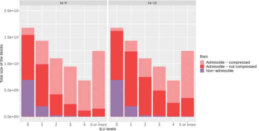
We first want to validate the hypothesis that using the fill-in levels is a good heuristic to classify the blocks based on their compressibility ratios. Figure 3 reports the accumulated memory consumption for all the 31 studied matrices in our experiments with three different tolerance criteria and by fill-in levels. The purple bars show the memory consumption of the structurally non-admissible blocks (too small to be compressed) and is stable for all precisions. The red part corresponds to the admissible blocks. The dark red is the memory footprint when they are compressed. It naturally increases with a more accurate tolerance. The light red shows the amount of memory that can be saved by compressing the blocks. One can observe that the lower the tolerance, the higher the gain.
These results show that the compression ratio of the admissible blocks in-creases with the levels. It confirms the original hypothesis, that fill-in levels can help to better tune the admissibility criterion in order to save flops for a small memory overhead. Furthermore, this parameter needs tuning to adapt to the tolerance. One can see that for a tolerance of 1e−12, only levels greater than 3 offer more than 50% memory savings, while all levels at 1e−4 almost reach 50%
10 Korkmaz & Faverge & Pichon & Ramet 1e−8 1e−12 0 1 2 3 4 5 or more 0 1 2 3 4 5 or more 0.0e+00 5.0e+09 1.0e+10 1.5e+10 2.0e+10 ILU levels T otal siz e of the b locks Bars Admissible − compressed Admissible − not compressed Non−admissible
Figure 3: Potential memory saving based on the tolerance criterion and fill-in levels. The bars report the cumulative memory of the 31 matrices. Purple represents the memory consumed by blocks below the size criteria, and red the memory of the admissible blocks for compression. Light red is the portion that can be saved when compressed.
savings. As a consequence, the fill-in level used to define the admissibility crite-rion will need to be adapted to both the tolerance and the maximum memory overhead defined by the user.
5.2
Comparison of the Costs
This section discusses the sequential experiments. Figure 4 shows the memory peak, factorization flops and factorization time profiles obtained for different precisions. We study the impact of the first fill-in levels (0 to 4) with respect to Minimal Memory (−1) and Just-In-Time (∞). Each curve represents the number of matrices within a percentage overhead of the best solution for each metric and matrix.
First, as expected, the lower the fill-in level chosen for admissibility, the lower the memory peak of the solver. One can observe that the impact of the fill-in level increases as the accuracy decreases. This confirms the trend already observed on Figure 3. ILU (∞) consumes up to 6.6 times more memory at 1e−4 while it drops to 3.4 times at 1e−12. Additionally, at this high tolerance, high levels of fill-in are able to reach the best memory peak. That means that potential flops reduction is possible without negatively impacting the memory.
Second, when observing the flop count evolution, the results are naturally reversed. The higher levels of fill-in are better to generate less flops. One can observe that for low accuracy (1e−4), a level of 0 is enough to reach the same flop count as the Just-In-Time scenario (ILU (∞)). When increasing the accuracy, more levels need to be considered admissible to lower the flop count to its minimal value. Except some corner cases, levels 1 or 2 are enough for
1e−8, and respectively 3 or 4 for 1e−12.
Finally, the time profiles follow the same trend as the flops profiles, with larger differences between the ILU (k) methods. This can be explained by the disparity of the LR2LR and LR2FR efficiency, as well as their variation in number that may increase the phenomena already observed on flops. Thus, one can observe that ILU (0) is the best average solution at 1e−4. It even outperforms the Just-In-Time strategy by a factor up 1.4x. To explain this performance, we recall that in the Just-In-Time strategy, many null-rank blocks are allocated and later compressed, while in the new ILU (k) heuristic they may never be allocated. Indeed, they are originally null blocks and at low precision they may receive only null contributions. Thanks to these savings, ILU (0) at this tolerance almost doubles the memory footprint in the worst case with respect to the Minimal Memory strategy, but it remains 0.23 times the memory consumption of the ILU (∞) and the full-rank versions.
1e-4 1e-8 1e-12
Memor y P eak Flops Time 0% 200% 400% 0% 200% 400% 600% 0% 200% 400% 600% 0 10 20 30 0 10 20 30 0 10 20 30
Overhead percentage wrt the optimal
Number of matrices ILU(-1) ILU(0) ILU(1) ILU(2) ILU(3) ILU(4) ILU( ∞ )
Figure 4: Memory peak, factorization flops and factorization time profiles of dif-ferent precisions with sequential runs. Each color stands for a difdif-ferent ILU (k) level. The x-axis shows percentages with respect to the best method for each metric and matrix, while y-axis represents the matrix count in accumulated way. The observations in higher precisions are similar to the low precision, but with higher fill-in levels. At 1e−8, only the levels above 1 compete with the Just-In-Time strategy in terms of time, as well as providing a controlled memory overhead with respect to the best solution.
solu-12 Korkmaz & Faverge & Pichon & Ramet
tion, which reduces the gain one can obtain on the memory footprint. However, solutions with level 1 is a good compromise at this precision as it gets similar memory footprints as ILU (−1) (up to 1.49x), while being up to 8.5 times faster.
Memory Peak 1e-4 1e-8 1e-12 lap120 Bum p_2911 Queen_4147 St ocF -1465 Long_Coup_dt0 Cube_Coup_dt0
atmosmodl atmosmodd atmosmodj Emilia_923 CurlCurl_4 CurlCurl_3 Fault_639 Transpor
t
Ser
ena
ML_Geer PFlow_742 Geo_1438 Hook_1498 RM07R bone010 boneS10 audikw_1 Flan_1565
fem_hifr eq_cir cuit matr5 dielFilt erV2clx dielFilt
erV3clx inline_1 ldoor
3Dspectr alw av e2 0.25 0.50 0.75 1.00 0.25 0.50 0.75 1.00 0.25 0.50 0.75 1.00 Memor y(me thod)/Memor y(FR) ILU(-1) ILU(0) ILU(1) ILU(2) ILU(3) ILU(4) ILU( ∞ ) Memory Peak 1e-4 1e-8 1e-12
ILU(-1) ILU(0) ILU(1) ILU(2) ILU(3) ILU(4) ILU( ∞ ) 0.25 0.50 0.75 1.00 0.25 0.50 0.75 1.00 0.25 0.50 0.75 1.00 Memor y(me thod)/Memor y(FR)
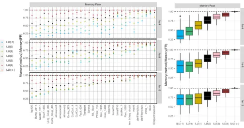
Figure 5: Memory peak ratio of the ILU (k) heuristic with respect to full-rank on the 31 test matrices. On the left, the detailed information is presented. On the right, the information is summarized with boxplots showing minimum, maximum, median, first quartile and third quartile of each level.
Figure 5 presents the detailed ratios of the memory peak of the different levels of admissibility with respect to the full-rank solution. One can observe that the Just-In-Time (ILU (∞)) strategy has the same memory peak as the full-rank version, and that the lower the level, the lower the memory peak. As we can observe all the matrices separately on the left, we can characterize them to decide which ILU (k) level is more convenient for each matrix to minimize the memory footprint. For example, one can see that, at 1e−12, the highest
level giving the minimal memory footprint is 1 for the first half, and 2 for the second half. These trends are similar on the flops and time figure showing that they are strongly connected. One can also observe, at 1e−4 that as mentioned above, increasing the level of admissibility seems to greatly increase the memory footprint with respect to the best one. However, it remains moderate when comparing with the full-rank implementation and it can be afforded to greatly reduce the time to solution.
The summary on the right of Figure 5 confirms the fact that the memory consumption increases with the higher fill-in levels and with the higher precision. The results at 1e−12 for the new heuristic at levels 1 and 2 show interesting results. As a matter of fact, they provide 25% memory improvement compared to the full rank version with equivalent time to solution. Note that, at this precision, even ILU (∞) does not manage to accelerate the full-rank version on the five most-right cases which do not compress at all. On the others, levels 1
and 2 are the best compromises since they are faster than the full-rank version while providing 25% memory saving in average.
To conclude, it is difficult to give one level as the optimal solution, but depending on the problem and the precision required, the level can be tuned to provide a solution that outperforms the Minimal Memory strategy in terms of time to solution for a small controlled memory overhead. Moreover, it can even have a speedup compared to the Just-In-Time strategy with less memory footprint.
5.3
Gain for the Multithreaded Version
This section presents the same experiments as in the previous section in a mul-tithreaded environment with 24 threads. Figure 6 presents the time profiles of the multi-threaded numerical factorization. Memory peak and flops are not reported as they are identical to the sequential ones.
We can observe that the effects already seen in sequential are also observed in a multi-threaded environment with a larger impact of the changes in the kernels (LR2LR or LR2FR). ILU (k) performs better with a level of 0, 2 and 4, for tolerances of respectively 1e−4, 1e−8, and 1e−12. Here, the Just-In-Time strategy is losing even more with respect to the ILU (k) strategy as it can be especially seen at 1e−4. In this case, we can also consider that the large memory reduction impacts the memory accesses of the threads. It helps ILU (0), which initially stores only the blocks of the original matrix A, to outperform the other versions. At 1e−12, one can observe that choosing ILU (2) is a good competitor
to ILU (∞), while saving 25% of memory in average.
1e-4 1e-8 1e-12
Time 0% 100% 200% 0% 100% 200% 300% 400% 0% 100% 200% 300% 400% 0 10 20 30
Overhead percentage wrt the optimal
Number of matrices ILU(-1) ILU(0) ILU(1) ILU(2) ILU(3) ILU(4) ILU( ∞ )
Figure 6: Time profiles of the multithreaded runs for different precisions. Each color shows a different ILU(k) level result.
6
Conclusion
The behavior of sparse supernodal direct solvers using low-rank compression highly depends on when the compression is performed. On one hand, all admis-sible blocks can be compressed before the factorization (as it happens with the
14 Korkmaz & Faverge & Pichon & Ramet
Minimal Memory strategy), allowing high memory savings at the cost of expen-sive low-rank updates. On the other hand, admissible blocks can be compressed after they have received all their updates (as for the Just-In-Time strategy), reducing significantly execution time with a controlled memory overhead.
In this paper, we proposed a new heuristic to estimate the compressibility of each block and constructed an algorithm that is a compromise between the two strategies mentioned previously. The new heuristic, named ILU (k), relies on the ILU fill-in levels to define an algebraic distance to compute low-rank admissibility of the blocks. The purpose of defining the admissibility was to propose an intermediate solution that accelerates the Minimal Memory solution while it slightly increases the memory consumption.
The experiments that we conducted on a large set of 31 real matrices demon-strated that our heuristic, ILU (k), manages to identify the low-rank blocks efficiently. The solution proposed runs up to 8.52 times faster than Minimal Memory with only a 1.49 times increase of memory usage for high precisions in both sequential and multi-threaded environments. Moreover, due to the elimi-nation of the null blocks before the numerical factorization, our new heuristic is able to run 1.4 times faster than the Just-In-Time strategy in sequential, with a much lower memory consumption (0.23 times less). In the multi-threaded environment, it even goes to 2.01 times faster for most of the cases. However, the best k value to use is not defined, even if clear trend appears.
For future work, we plan to introduce tuning techniques to automatically infer the best value of k depending on the properties of the machine used and the tolerance given. An orthogonal work of this paper consists in exhibiting more regular sparse structures, gathering unknowns that receive similar contributions (and thus have the same fill-in level). It could be done for instance by aligning separators, as presented in [20].
Acknowledgments
This work is supported by the Agence Nationale de la Recherche, under grant ANR-18-CE46-0006 (SaSHiMi). Experiments presented in this paper were car-ried out using the PlaFRIM experimental testbed, supported by Inria, CNRS (LABRI and IMB), Universit´e de Bordeaux, Bordeaux INP and Conseil R´egional d’Aquitaine (https://www.plafrim.fr/).
References
[1] Amestoy, P.R., Ashcraft, C., Boiteau, O., Buttari, A., L’Excellent, J.Y., Weisbecker, C.: Improving Multifrontal Methods by Means of Block Low-Rank Representations. SIAM Journal on Scientific Computing 37(3), A1451–A1474 (2015)
[2] Amestoy, P.R., Buttari, A., L’Excellent, J.Y., Mary, T.: On the complexity of the block low-rank multifrontal factorization. SIAM Journal on Scientific
Computing 39(4), 1710–1740 (2017). https://doi.org/16M1077192, https: //oatao.univ-toulouse.fr/19066/
[3] Amestoy, P.R., Buttari, A., L’Excellent, J.Y., Mary, T.: Bridging the gap between flat and hierarchical low-rank matrix formats: the multilevel BLR format. SIAM Journal on Scientific Computing 41(3), A1414–A1442 (May 2019)
[4] Aminfar, A., Darve, E.: A fast, memory efficient and robust sparse pre-conditioner based on a multifrontal approach with applications to finite-element matrices. International Journal for Numerical Methods in Engi-neering 107(6), 520–540 (2016)
[5] Campbell, Y., Davis, T.A.: Incomplete lu factorization: a multifrontal approach. https://ufdcimages.uflib.ufl.edu/UF/00/09/53/48/00001/1995185.pdf (October 1995)
[6] Chadwick, J.N., Bindel, D.S.: An Efficient Solver for Sparse Lin-ear Systems Based on Rank-Structured Cholesky Factorization. CoRR abs/1507.05593 (2015)
[7] Davis, T.A., Hu, Y.: The University of Florida sparse matrix collection. ACM Trans. Math. Softw. 38(1), 1:1–1:25 (Dec 2011). https://doi.org/10.1145/2049662.2049663
[8] Dongarra, J., Du Croz, J., Hammarling, S., Duff, I.S.: A set of level 3 basic linear algebra subprograms. ACM Trans. Math. Softw. 16(1), 1–17 (1990) [9] Duff, I.S., Erisman, A.M., Reid, J.K.: Direct methods for sparse matrices.
Clarendon Press (1986)
[10] Ghysels, P., Li, X.S., Rouet, F.H., Williams, S., Napov, A.: An Effi-cient Multicore Implementation of a Novel HSS-Structured Multifrontal Solver Using Randomized Sampling. SIAM Journal on Scientific Comput-ing 38(5), S358–S384 (2016)
[11] Hackbusch, W.: A Sparse Matrix Arithmetic Based on H-Matrices. Part I: Introduction to H-Matrices. Computing 62(2), 89–108 (1999)
[12] Hackbusch, W.: Hierarchical Matrices: Algorithms and Analysis, vol. 49 (12 2015). https://doi.org/10.1007/978-3-662-47324-5
[13] Hackbusch, W., B¨orm, S.: Data-sparse Approximation by Adaptive H2
-Matrices. Computing 69(1), 1–35 (2002)
[14] H´enon, P., Ramet, P., Roman, J.: On finding approximate supernodes for an efficient block-ilu(k) factorization. Parallel Computing 34(6), 345–362 (2008). https://doi.org/https://doi.org/10.1016/j.parco.2007.12.003, https://www.sciencedirect.com/science/article/pii/
16 Korkmaz & Faverge & Pichon & Ramet
[15] Hysom, D., Pothen, A.: A scalable parallel algorithm for incomplete factor preconditioning. SIAM J. Sci. Comput. 22, 2194–2215 (2001)
[16] Karypis, G., Kumar, V.: Parallel threshold-based ilu factorization. pro-ceedings of the IEEE/ACM SC97 Conference (1997)
[17] Liz´e, B.: R´esolution directe rapide pour les ´el´ements finis de fronti`ere en ´electromagn´etisme et acoustique : H-matrices. parall´elisme et appli-cations industrielles. Ph.D. thesis, ´Ecole Doctorale Galil´ee, Paris, France (Jun 2014)
[18] Marchal, L., Marette, T., Pichon, G., Vivien, F.: Trading Performance for Memory in Sparse Direct Solvers using Low-rank Compression. Re-search Report RR-9368, INRIA (Oct 2020), https://hal.inria.fr/ hal-02976233
[19] Mary, T.: Block Low-Rank multifrontal solvers: complexity, performance, and scalability. Ph.D. thesis, Toulouse University, Toulouse, France (Nov 2017)
[20] Pichon, G.: On the use of low-rank arithmetic to reduce the complexity of parallel sparse linearsolvers based on direct factorization technique. Ph.D. thesis, Universite de Bordeaux,, Bordeaux, France (2018)
[21] Pichon, G., Darve, E., Faverge, M., Ramet, P., Roman, J.: Sparse supern-odal solver using block low-rank compression: Design, performance and analysis. International Journal of Computational Science and Engineering 27, 255 – 270 (Jul 2018)
[22] Rose, D.J., Tarjan, R.E.: Algorithmic aspects of vertex elimination on directed graphs. SIAM J. Appl. Math. 34(1), 176–197 (Jan 1978). https://doi.org/10.1137/0134014
[23] Saad, Y.: Iterative Methods for Sparse Linear Systems. Society for Indus-trial and Applied Mathematics, USA, 2nd edn. (2003)
[24] Watts, J.W.: A conjugate gradient truncated direct method for the iterative solution of the reservoir simulation pressure equation. Society of Petroleum Engineers Journal 21, 345–353 (1981)
[25] Xia, J.L.: Randomized sparse direct solvers. SIAM Journal on Matrix Anal-ysis and Applications 34(1), 197–227 (2013)
200 avenue de la Vieille Tour 33405 Talence Cedex
BP 105 - 78153 Le Chesnay Cedex inria.fr