Control of a dual inverted pendulum system using linear-quadratic and H-infinity methods

Control of a Dual Inverted Pendulum

System

Using

Linear-Quadratic

and H-Infinity

Methods

by

Lara C. Phillips

B.S., University of Missouri - Rolla

(1991)

Submitted to the Department of

Electrical Engineering and Computer Science

in Partial Fulfillment of the Requirements

for the Degree of

Master of Science

in Electrical Engineering

at the

Massachusetts

Institute

of Technology

September

1994

© Massachusetts Institute of Technology, 1994.

All Rights Reserved

Signature of Author

I V I ~ __ . *---

Department of Electrical Engineering

and Computer Science

June 10, 1994 Certified by

,-\

Michael Athans

Thesis Supervisor

) ,

Control of a Dual Inverted Pendulum

System

Using

Linear-Quadratic

and H-Infinity Methods

by

Lara C. Phillips

Submitted to the Department of Electrical Engineering and

Computer Science on June 10, 1994, in partial fulfillment of the requirements for the Degree of Master of Science.

Linear-Quadratic Regulator (LQR) and H-Infinity (H) with full state feedback design methods are applied to a cart with two inverted

pendulums attached, named a dual inverted pendulum system.

A

linearized model of the system is obtained, and its open-loop properties are examined. The LQR and H design methods are applied to the system with the objective of stabilizing it and

approximately maintaining the open-loop bandwidth.

The methods

are applied to the dual inverted pendulum system for two different ratios of rod lengths to see the differences in the closed-loop

responses. With the H design method, frequency weighting the

control is needed to shape the frequency response to meet the bandwidth constraint. The LQR and frequency weighted H. designs are compared in both the time and frequency domains. These

comparisons indicate that the closed-loop systems have satisfactory

transient responses (not always the case for the H_ designs), stability

robustness, and bandwidth, but amplify the disturbances in some

frequency ranges.

Thesis Supervisor: Dr. Michael Athans

Acknowledgments

I would first like to thank my family for their encouragement

and support during my three years at M.I.T. I would especially like to thank my dad, for instilling in me the confidence and courage to attend graduate school, and for his "gentle prodding" to attend M.I.T. I would also like to thank Professor Michael Athans, first, for

suggesting the topic of this thesis, and second, for his guidance,

support, and patience as my thesis advisor. In addition, I would like to express my appreciation to some of the members of the LIDS group, namely Stephen Patek, Leonard Lublin, and Alan Chao, for

taking the time to answer questions pertaining to my thesis.

Thanks must also go to my friends, both old and new, who have

provided much support throughout my stay at M.I.T. Special thanks

go to the following three people: Jennifer (Reed) Barney, my best friend since the second grade, for always listening and cheering me

up during our (ahem) hour-long phone conversations; Birgit

(Kuschnerus) Sorgenfrei, my first and closest friend at M.I.T., for

sharing in the teaching and M.I.T. experiences; and John Shirlaw, my English friend, for offering new and interesting views on life, once I was able to translate them from "English" to "American". Thanks also go to S.S., L.A., F.F., L.H., N.P. (Ashdowners), K.C., J.B., D.L., M.S. (TAs), and B.R., D.J. (MCS survivors).

Table of Contents

Chapter

1.1

1.2

Chapter

2.1

2.2

Chapter

3.1

3.2

3.3

1

Introduction

Background

...

Thesis Overview...

2 The Dual Inverted Pendulum System

State Space Representation ...

Open-Loop Analysis ...

2.2.1 Open-Loop Poles and Zeros ...

2.2.2 Controllability and Observability ...

2.2.3 Open-Loop Frequency Responses...

3

Chapter 4

4.1

4.2

4.3

Linear-Quadratic Regulator Design

LQR Methodology....

...

LQR Design ...

LQR Closed-Loop Simulation Results ...

3.3.1 LQR Time Response...

3.3.2 LQR Frequency Response ...

Page

8 8 9

12

12

15

15

19

21

24

24

26

28

28

30

H-Infinity with Full State Feedback Design

3 3

H

with Full State Feedback Methodology ...

33

H_ with Full State Feedback Design ... 35

H.

Closed-Loop Simulation Results ...

36

H, with Full H. with Full Response ...

State Feedback

State Feedback

.. *. . . . .

Time Response ..

Frequency

. . . .

4.3.1

4.3.2

36

38

Table of Contents (cont.)

Page

4.4

Frequency

Weighting

Methodology

...

4.5

Frequency Weighted H, Design ...

4.6

Frequency Weighted H. Closed-Loop

Results

...

Simulation

4.6.1 Frequency Weighted H.

Time Response...

4.6.2 Frequency Weighted

Chapter 5

H.. Frequency

Design Comparisons

5.1

Time Response ...

5.2

Frequency

Response

...

5.3

Parameter Variation ...

Chapter

6 Conclusions

Future Work

and Suggestions

for

58

6.1

Conclusions ...

6.2

Suggestions for Future Work ...

Appendix

A

Appendix B

Appendix

C

State Space Representation

Open-Loop Poles and Zeros

Controllability and Observability

58

60

61

66

71

Additional Time Responses

39

42

44

44

Response .

46

49

49

52

54

78

List of Figures

Page

2.1 The Dual Inverted Pendulum System ... 1 3 2.2 Open-Loop Pole and Zero Locations, T(s) ... 1 8 2.3 Open-Loop Pole and Zero Locations, T,(s) ... 1 8

2.4

Open-Loop Pole and Zero Locations, Ty(s) ...

....

19

2.5 Open-Loop Pole and Zero Locations as the Length of the Longer Rod is Decreased ... 20

2.6 Open-Loop Frequency Response, Control to Rod Angles ... 22

2.7

Open-Loop Frequency Response, Disturbances to Cart

Position ...

23

3.1

LQR Implementation ...

26

3.2 LQR Time Response, x(0)=[1 0 0 0 0 0] ... 29

3.3

LQR Complementary Sensitivity ...

30

3.4 LQR Disturbance Rejection, Tf,y(s) ... 31

3.5 LQR Disturbance Rejection, Tfy(s) ... 31

4.1 H. Time Response, x(0)=[1 0 0 0 0 0] ... 37

4.2

H_

Complementary Sensitivity ...

38

4.3

Frequency Weighting Function and Frequency Domain

Result

...

...

...

39

4.4 Frequency Weighted

H

Implementation ...

41

4.5

Preliminary H Control Weighting ...

42

4.6

Final H. Control Weighting, System 1 ...

43

4.7 Final H_ Control Weighting, System 2 ... 43

4.8 Frequency Weighted H Time Response, x(0)=[1 0 0 0 0 0] ... 45

4.9

Frequency Weighted H Complementary Sensitivity ...

4 6

4.10 Frequency Weighted H Disturbance Rejection, Tf,l(s) ....

47

List of Figures (cont.)

4.11 Frequency Weighted H Disturbance Rejection, T,(s) ....

5.1 Time Domain Comparison, System 1,

x(O)=[1 o0 0 0 0] ...

5.2 Time Domain Comparison, System 2,

x(0)=[1 0 0 0 0 0] ...

5.3

Complementary Sensitivity Comparison ..

5.4

Disturbance Rejection Comparison, System

5.5

Disturbance Rejection Comparison, System

5.6

Parameter Variation Comparison, System

5.7

Parameter Variation Comparison, System

A.1 The Dual Inverted Pendulum System ...

A.2 Diagram for Force Equation ...

A.3 Diagram for Moment Equations...

C.1 Open-Loop Pole and Zero Locations

Longer Rod is Decrease

D.I Time Response, System Response, Response, Response, Response, Response, Response, Response, System System System System System System System

d ...

1, x(0) [O 2, x(0) = [0 1, x(O) = [0 2, x(0) = [0 1, x(0) = [1 2, x(0) = [1 1, x(0) = [1 2, x(0) = [1 1 ....· ·...

2...

I ...

2··....·...

as the Length of the

.. .. .. . . . . 0 0 0] ... 0 0 0 0 ... 0 0 0 O] ... 0 0 0 O] ... 0 1' 0 -1' 0] ... 0 -1' 0 -1 O] ... 0 1' 0

-

01 ] ... 0 1' 0 -1 01 ] ...

Page

48

50

51

52

53

54

56

57

61

62

62

74

79

80

81

82

83

84

85

86

D.2 D.3 D.4 D.5 D.6 D.7 D.8

Time

Time

Time

Time

Time

Time

Time

Chapter

1

Introduction

In this chapter, the background and outline of this thesis are

presented.

1.1

Background

The single inverted pendulum system is often used in classical

controls classes to demonstrate the stabilization of an open-loop

unstable system, and has also been used in demonstrating the design

of intelligent integral control [1], the dynamic principle of parametric

excitation, and the considerations and problems involved in actually

constructing such a system [2], [3]. A more interesting and

complicated problem in terms of controller design is the dual

inverted pendulum system, in which there are two inverted

pendulums on one cart. This system has an additional unstable pole and nonminimum phase zero in the open-loop plant than the single

inverted pendulum system and is therefore more difficult to

stabilize.

Systems with open-loop plants containing unstable poles and

nonminimum phase zeros can be stabilized using constant gain

feedback controllers, such as those that result from the

compensators that might result from Linear-Quadratic Gaussian

(LQG) or H.-Optimization design methodologies. However, even

though the unstable, nonminimum phase systems are stabilized using

the above design methodologies, the closed-loop systems generally

exhibit poor performance characteristics such as sensitivity to

parameter value variations and disturbance amplification in some

frequency ranges [4].

Stabilization of the dual inverted pendulum system is

demonstrated using the LQR and H with full state feedback design methodologies. Each design is realized for two different ratios of rod lengths. System 1 represents the system with a ratio of 16:1 for the rod lengths, and System 2 represents the system with a ratio of 2:1. The controllers are designed such that the bandwidths of the

open-and closed-loop systems are comparable.' The closed-loop systems

for each design methodology are compared in both the time domain

and frequency domain, comparing such design characteristics as

transient response, stability robustness, and disturbance rejection

properties, and in the sensitivity of the closed-loop system to

parameter variations.

1.2

Thesis Overview

locations, controllability and observability, and frequency responses,

are also investigated. The open-loop pole and zero locations for specific transfer functions are given, and the derivations of the locations are presented in Appendix B. The controllability and observability properties of the system are discussed, and the

equations providing the results are included in Appendix C. Finally,

specific transfer functions are examined in the frequency domain.

Chapter 3 presents the design methodology for the

linear-quadratic regulator (LQR). The effect of the control weighting coefficient on the closed-loop poles is discussed, and a value is

determined to satisfy the bandwidth constraint.

Time and frequency

responses of the closed-loop system are shown.

Chapter 4 presents the H with full state feedback design methodology. It is found that the H with full state feedback

controller does not meet the bandwidth constraint. To reduce the

bandwidth, the control is frequency weighted. The method of

frequency weighting is presented, and a frequency weighting is

determined for which the bandwidth constraint is better satisfied.

Time and frequency responses of this closed-loop system are also

shown.

In Chapter 5, the two design methodologies are compared for

both System 1 and System 2. The designs are compared in the time

domain in terms of the amount of the perturbations from

equilibrium, the magnitude of the necessary control, and the

transient times. Time responses for several initial conditions are

shown in Appendix D. In the frequency domain, the stability

final design comparison involves a parameter variation, in which the

length of the longer rod is varied until the closed-loop systems again

become unstable.

Chapter 6 briefly summarizes the conclusions, and

recommendations for future research are given.

Complete

appendices and selected references are included at the end of the

Chapter 2

The Dual Inverted Pendulum System

In this chapter, the state space representation of the dual

inverted pendulum system is presented, and properties of the

open-loop system are examined.

2.1

State Space Representation

The first step in analyzing any system is to obtain a

representation of its dynamics. For many design purposes, a linear

representation about an equilibrium point is sufficient to obtain a

good controller. A linear model of the system can be obtained from

the nonlinear dynamic equations which describe the system by

establishing the steady-state equilibrium conditions, defining the

perturbations about this equilibrium point, introducing the

perturbations into the nonlinear equations, and then retaining only

the linear terms.

The state and output perturbation dynamics can

then be expressed in the standard state space representation form

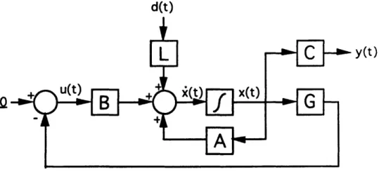
&(t) = A&(t) + B6u(t) + Ld(t), By(t) = CMx(t) + D6u(t) [5].

The derivation of the state space representation for the dual

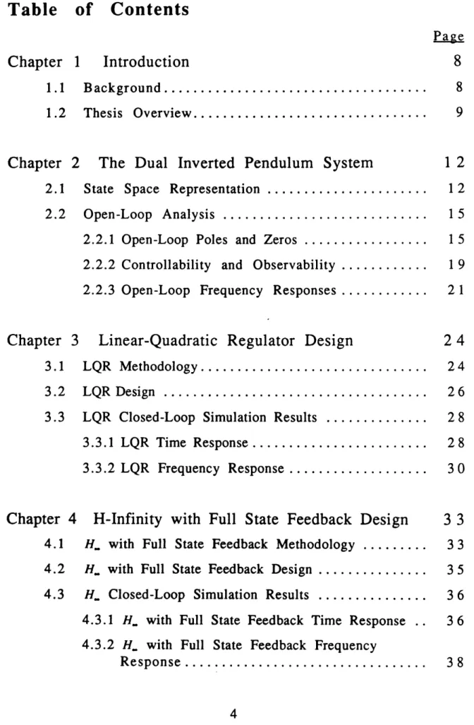
inverted pendulum system of Figure 2.1 is included in Appendix A.

The assumptions for finding the nonlinear equations describing the

attached to the cart with frictionless pivots; the gravitational field is

uniform; the disturbances can be modeled as forces acting on the tips of the rods; and the control for the system is a translational force acting on the cart. We also assume that all of the states can be

measured without sensor noise (i.e., we have full-state feedback),

and that the position of the cart from some reference point is the

state variable we want to control.

f,(t)

m

2

2t2

Figure 2.1 The Dual Inverted Pendulum System

In Figure 2.1, M is the mass of the cart, 21, and 212 are the

In Appendix A, the state, control, and disturbance vectors are defined to be: 8x(t) = 8z(t) 8&(t)

80,

(t) 8o1(t)

8,

2

(t)

462

(t)-8u(t)= [f(t)]

d(t) = [ (f (t)]

perturbed cart position (m) perturbed cart velocity (m / s)

perturbed angular position of the shorter rod (rad) perturbed angular velocity of the shorter rod (rad / s) perturbed angular position of the longer rod (rad) perturbed angular velocity of the longer rod (rad / s)

perturbed control force (N)

perturbed disturbance force on the shorter rod (N) perturbed disturbance force on the longer rod (N)

and the state space representation for the dual inverted pendulum

system is shown to be

0

1

0

o O -3M,g

z

00 0 o 0 3g(Z+3M) 4Zh 00 O o o 9Mg 4ZI2 0 0 o -3M~g

z

1 0 0 9M2g 4Z1, 0 0 0 3g(Z + 3M) 4Z4 0 0 0 0 1 0 6x(t) + 0 4 Z 0 -3 ZI, O -3

.zA

y(t)=[1 0 0 0 0 O]6x(t)

where

M = 2rnl1, M2= 2 212, and Z = 4M + Ml + M2.

i()

=

8u(t) + 0 -2 Z 3(M, + Z) 2M,I,Z 0 3 2Z12 0 -2

z

0 3 2Z11 0 3(M2 + Z) 2M22Z 6d(t)

(2.1)

In subsequent chapters, the 6's are omitted from the equations

and the state space representation is written as

i(t) = Ax(t) + Bu(t) + Ld(t)

(2.2)

y(t) = Cx(t)

2.2

Open-Loop Analysis

The open-loop analysis of the dual inverted pendulum system

involves finding open-loop pole and zero locations in terms of the

system parameters, investigating the controllability and

observability of the system, and examining such transfer functions as

the control to the angles of the rods, and the disturbances to the cart

position.

2.2.1

Open-Loop Poles and Zeros

The open-loop pole and zero locations of the dual inverted pendulum system from the control to the cart position (from u to y)

can be found from the open-loop transfer function T(s)=C(s

-

A)-'B.

Because the system is SISO (single input, single output), the poles are

the roots of the denominator of the transfer function and the zeros

are the roots of the numerator. From the transfer function,

8

+3

+

2 ]

]

(z)[+3M[

Z 3M2 ( 2 )(2.3)

and the open-loop zero locations are:

(g,

3{g (2.4)

There are two open-loop poles at the origin and the other four poles are symmetric about the ji-axis. Because of the poles in the

right-half plane, the system is unstable. The four open-loop zeros

are also symmetric about the jw-axis. The zeros in the right-half plane cause the system to be nonminimum phase. The magnitudes of

the zeros are the natural frequencies of the individual rods.

Note that the poles are dependent on the masses of the cart and the rods. Increasing the mass of the cart or the masses of the

rods pushes the non-zero poles farther away from the j-axis,

causing the system to become harder to control. Physically, the heavier a cart is, the harder it is to move back and forth, and the heavier an inverted rod is, the more difficult it is to keep vertical.

The open-loop pole and zero locations from the disturbances to the cart position (f, and f2 to y) can be found from the transfer

functions T,(s)=C(sl-A)-'L,

and T,,(s)=C(sI- A)-

1

L,

respectively,

with the disturbance matrix L rewritten as L=[L, L]. Since the poles depend only on the A matrix, these transfer functions have the same pole locations as given in (2.3). The transfer functions are included in Appendix B, and the zeros are found to be:

zeros of Tf,(s):

±+

,

±jg

(2.5)

zeros of

T(s):

+±

4(

i

j

2(2

(2.6)

Note that these transfer functions have real and complex zeros. If a disturbance force is of a frequency equal in magnitude to its respective complex zero, the rod oscillates at the same frequency in such a way that the cart does not "see" the disturbance, and

therefore does not move [5], [6].

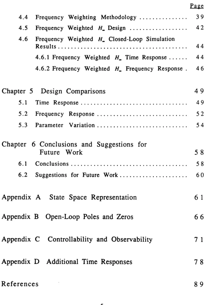
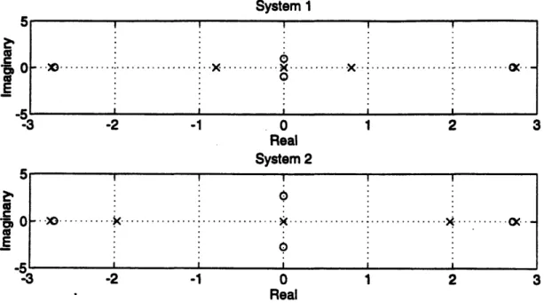
The open-loop pole and zero locations for the three transfer functions mentioned above are given below for System I and System 2, and are also shown in Figures 2.2, 2.3, and 2.4.

SYSTEM 1: l, =lm,1 2=16m: open-loop poles: 0,0, + 2.7485, ± 0.8022 zeros of T(s): 2.7130,±0.6783 zeros of Tfy(s): 0.6783,±j3.8368 zeros of Tf2(s):

±2.7130,

jO.9592 SYSTEM 2: =lm, l2 =

2m:

open-loop poles: 0,0, + 2.7545, ±1.9703 zeros of T,y(s):

±2.7130,1.9184

zeros of Tf,(s): +1.9184,+j3.8368 zeros of Tf2y(s): +_2.7130,±j2.7130

System 1 I I I I I

... x ...

0 Real System 2 1

x

0

i I 0 Real 1

Figure 2.2 Open-Loop Pole and Zero Locations, T(s)

System 1 -3 -2 -1 0 1 2 Real System 2 5 _ I I 0I I _ -3 -2 -1 0 Real 1

Figure 2.3 Open-Loop Pole and Zero Locations, 2 1 0 C

.0

E 0

- .0...

_'1 -I -3 -2 -1 1 C: E 0

-

.)0... 2 3 _1

0·

.)

.... -2 -I -3 -1 2 3 .' co 0_C 0 co E a% 0 to 0 E 3 Tf,,(S) ..: ... (X. I -I · · · X·O·· ... ox ... · . .: . . . . I -... k ... I . . . . I I I 3

System 1 0 cao C E _0 '3 -2 -1 0 1 2 3 Real System 2 0 co ' 0 co E _AI · 3 -2 -1 0 1 2 3 Real

Figure 2.4 Open-Loop Pole and Zero Locations, T,y(s)

2.2.2

Controllability and Observability

The controllability and observability of the dual inverted

pendulum system are also considered because if a system is not

controllable and observable, it is meaningless to search for an

optimal controller.

Because the system contains unstable modes, we

are actually looking at the stabilizability and detectability properties

of the system.

For a system to be controllable, for any initial state and any

I_1

i

,

I I i , . . i -.. > ... o ... ... .... X-xo--. 0 I I I

unstable modes is said to be stabilizable and detectable if the

unstable modes are controllable and observable, respectively [5].

The controllability and observability properties of the dual inverted

pendulum system are examined in Appendix C in terms of the

system parameters in the controllability and observability matrices.

The loss of controllability and/or observability can also be

caused by a pole/zero cancellation. In Figure 2.5, the open-loop pole and zero locations are shown as the length of the longer rod, l2, is

decreased to equal the length of the shorter rod, 1l. The plot

indicates that when the rods are of equal length there are pole/zero cancellations at 2.7130 (two zeros and one pole at each). A pole/zero

cancellation implies a loss of controllability and/or observability. To

determine which loss the system experiences, the mode and the pole

and zero "directions" must be examined. The loss of controllability

and observability for this pole/zero cancellation is also discussed in

Appendix C, along with an examination of other possible cases which

Length of Shorter Rod, 11, Equals 1

m 15P ) ... - x... .x ... X ... o x .: .o° . .--. - :X) xo X ox oC ) o : :XO X OX: C X) xo x Ox CO( )O XO X OX O( X:) NO X OX: OC

510

-) ...

.. .

... ...

...

c )O XO X OX (X X) )O X 0 (X )G -O D - 0Cc -3 -2 -1 0 1 2 3 Real Axis

Figure 2.5 Open-Loop Pole and Zero Locations as the Length of the Longer Rod, 12, is Decreased

give a cancellation. It is found, however, that the system loses controllability and observability only when the lengths of the rods are equal, and that the system cannot lose only one or the other.

The fact that the dual inverted pendulum system is both uncontrollable and unobservable when the rods are equal in length makes sense physically. The uncontrollability of the system can be thought of in this way: rods of equal length oscillate at the same frequency, 3ig , so that if they are started with the initial

condition 08(0) =

-02(0),

the final condition of 0,(T)= 02(T) can not be reached for any control u(t), and thus the system is uncontrollable.

The unobservability of the system can be reasoned as follows: with the same initial conditions as above, the rods exert equal and

opposite forces on the cart when they fall, and therefore the cart does not move. However, since a net force of zero results on the cart

for several initial conditions ((0)=10'=-02(0)

or

90(0)=-5

=-02(0), for

example), the system is unobservable.

2.2.3

Open-Loop

Frequency

Responses

Finally, we examine some open-loop transfer functions of the

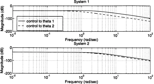
dual inverted pendulum system. The transfer functions shown in Figure 2.6, the control to the angles of the rods for System 1 and System 2, indicate that we can control the angle of the shorter rod,

System 1 I' -control to theta 1 . ... - control to:theta 2.... 102 10'100 10' 10 102 Frequency (rad/sec) System 2 A CU

_I..

._n . . . . ii... . . . . .ii . . . . .il . . iiii

10' 10' 100 101 102

Frequency (rad/sec)

Figure 2.6 Open-Loop Frequency Response, Control to Rod Angles

horizontal movement at the base of a shorter rod causes a larger

angular deflection of the tip than if the same horizontal movement is

applied to a longer rod.

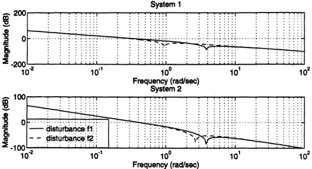
The transfer functions in Figure 2.7, the disturbances to the

cart position, show that disturbances greatly affect the position of the

cart at the lower frequencies. The plots also reveal the fact that

there are complex zeros for these transfer functions (refer to (2.5)

and (2.6)). It appears from Figure 2.7 that if the disturbance is of a frequency equal in magnitude to that of a complex zero, the

disturbance has less effect on the position of the cart than at many of the other frequencies. These slight dips in the responses should

System 1

....::

:

. .... ... ... ... .... ...

.

....

.

. .iiiiii

...

....

... ii . .i . . . ...

.~~~~K

. ... ...

100 Frequency (rad/sec) System 2 100 Frequency (rad/sec) 101 101

Figure 2.7 Open-Loop Frequency Response, Disturbances to Cart Position

the disturbance is of a frequency equal in magnitude to that of a complex zero, the cart does not move.

Now that the open-loop properties of the dual inverted

pendulum system have been examined, the LQR

and H.

compensators can be designed.

20( -20C 1 loC C 0'-2 0 m c -0 V .₀ m

.1

co la .8 10'1 10' 1 1: .1 AC .. .... ... -isturbae .. ... 10 O 1( )2 11

Chapter

3

Linear-Quadratic

Regulator Design

The linear-quadratic regulator design methodology is

presented in this chapter, and a controller is designed for the dual

inverted pendulum system.

The closed-loop time and frequency

responses are also examined.

3.1

LQR Methodology

The linear-quadratic regulator (LQR) method is used to design a linear controller for a system with full state feedback. The LQR

design method develops controllers for systems of the form

x(t) = Ax(t) + Bu(t), x(O) = x, x(t)E 1, u(t) e 9

[A,B] stabilizable (3.1)

which minimize the cost performance

J = i[x'(t)Qx(t)

+ u'(t)Ru(t)]dt

(3.2)

where Q is the symmetric, positive semidefinite state weighting

matrix, and R is the symmetric, positive definite control weighting

matrix. It is also necessary that [A,Q

1 2

_{] is detectable.}

The solution of the regulator problem is a time varying control

law which in steady-state becomes the linear time-invariant, state

feedback law [6], [7]:

u(t) = -Gx(t) (3.3)

where G is the (mxn) control gain matrix given by

G = R-'B'K (3.4)

and K is the unique symmetric, positive semidefinite (n x n) solution

of the algebraic Riccati equation

KA + A'K + Q - KBR-B'K = 0 (3.5)

The control law defined by (3.3) is unique and minimizes the

cost functional, provided that the stabilizability and detectability

conditions are met. If there are input disturbances to the plant, the

optimal controller is determined as above, ignoring the fact that

there are disturbances, and it is implemented as shown in Figure 3.1

d(t)

y(t)

Figure 3.1 LQR Implementation

3.2

LQR Design

As mentioned in Chapter 2, the state variable we want to

control is the position of the cart from a reference point. Therefore,

in the LQR cost performance of (3.2), the state weighting matrix Q

equals C'C.

The controllers are to be designed such that the open- and closed-loop bandwidths are comparable. With LQR control, if we let

R=pl,p>O in the cost functional, then as p-0, some of the closed-loop poles go to cancel any minimum phase zeros, or go to the mirror

image, about the jw-axis, of any nonminimum phase zeros of the

open-loop system, and the rest go off toward infinity along stable

Butterworth patterns [7]. Thus, we can vary the value of p to obtain

closed-loop poles within the same distance from the origin of the

s-plane as the open-loop poles. From the locations of the open-loop

poles for System 1 (0,0,+2.7485,+ 0.8022) and System 2

(0,0,±2.7545,+1.9703), it is decided to have the closed-loop poles inside a semicircle of radius three from the origin.

The value of p is varied until the closed-loop poles that are heading off toward infinity from the origin along stable Butterworth

patterns are just inside the radius of three semicircle. The other

closed-loop poles head toward minimum phase and "mirror-image"

nonminimum phase zeros, which are inside the pole locations (Figure

2.2). The value of p and the closed-loop pole locations for System 1 and System 2 are as follows:

System 1:

p = 0.000353

closed-loop poles: -2.1564 ± j2.0852,- 2.7268 + jO.0175, -0.6785 + jO.0070,

System 2:

p = 0.000448

closed-loop poles: -2.1574 + j2.0831, - 2.7285 + jO.0204,

-1.9264 + jO.0193

Recall that the open-loop zero locations for System 1 and System 2 are ±2.7130,±0.6783 and ±2.7130,±1.9184, respectively. Thus we can see that four of the closed-loop poles are almost canceling the

minimum phase and "mirror-image" nonminimum phase zeros of the

open-loop system.

3.3

LQR Closed-Loop Simulation Results

The LQR closed-loop system has the form

.(t) = (A - BG)x(t) + L(t), x(O) = xo

y(t) = Cx(t) (3.6)

From these equations we can examine the time and frequency

responses.

3.3.1

LQR Time Response

From the locations of the closed-loop poles, we would expect System 2 to have a faster transient response than System 1. Time responses for System 1 and System 2 are shown in Figure 3.2. For this simulation it is assumed that only the cart has an initial

perturbation, equal to one meter, and that there are no disturbance

forces acting on the rods.

First notice from Figure 3.2 that System 2 does in fact have a

faster transient response.

The figure also indicates that System 1

experiences the largest perturbation of the cart from equilibrium,

and that the angle of the longer rod for System 2 deviates farther

from equilibrium than for System 1. The perturbation of the angle

makes sense physically because, as mentioned previously, a

horizontal movement at the base of a shorter rod causes a larger

angular deflection of the tip than if the same horizontal movement is

E .o CL 0 0 CL Time (sec) 10 -10 0 1 2 3 4 5 6 7 E Time (sec) 5 O

-5 _

l

' i

i

i

0 1 2 3 4 5 6 7 8 Time (sec) -50 n50! 0 ! ! ! .50

Ann~~~~~~~~~~~~~~~~~~~~~~~~~~~~

... ... ... ... ... 5c C -5C -10c 0.1 0.2 0.3 0.4 0.5 0.6 0.7 0.8 0.9 1 Time (sec) I c I g z '9 9 C 9 0 ! ! ! ! ! '" ' ! ·

...

i...i ... ... ... ...

...

... ...

I i I I I 3 '--0 D I )

Chapter 5 when the LQR design is compared to the frequency

weighted H design.

3.3.2

LQR Frequency Response

The frequency responses examined relate to stability

robustness and disturbance rejection. These are shown in Figures 3.3 and 3.4. The complementary sensitivity plot, Figure 3.3, is the

frequency response of the closed-loop transfer function matrix,

C,(s)=[I+G,(s)]

-G,(s), where G(s)=G(sI-A)-'B

1

is the loop transfer

function matrix and G is the control gain matrix of (3.4). With the

modeling errors reflected to the plant input, Figure 3.3 indicates that

the system can tolerate multiplicative errors with

a[E(jo)]<2,

for all

w (peaks are less than 6dB=201og(2)) [7].

m '5 g 0 h.. 10 10" ' 10° 101 102 -Frequency (rad/sec)

Figure 3.3 LQR Complementary Sensitivity

The disturbance rejection plots of Figures 3.4 and 3.5 show the

frequency responses of the open-loop and closed-loop transfer

System 1 200 -2 .1 00101 102 103 104 Frequency (rad/sec) System 2

i~~~~~~~~~~~~~~~~~~·~~~

-

i

_{_}

i i i--i

. :

=i.200.

i : i;;~;;; i ~ i~ii

i1 i i~;

1;~;::::::,

:..

10

'2

_{1 0 "}

₁₀

_{1 0 102}

°

_{103 104}

Frequency (rad/sec) System 2

== °l"'"i'i'i0iiifi i'~'Ti~i'~i":.!" ... . .. ... . f . i'"i"!'i'i'i'!~

0

F~/

7

:::: ::::::::

--

''"-~';-~-ii!~i

~E, n~ i ii ii; i ii iii i

t~l i ~ ; i i ii;: : fii

-d..vo _{10-2 10'} -1 _{1 10 102 103 10}4

Frequency (rad/sec)

Figure 3.4 LQR Disturbance Rejection, Tf,y(s)

System 1 200. 0 _{. . ..}

L~~...

:'::::: i!!i:i

t

~

; ;

;~;~;;i

::i:

:,

~:

~

0200 10'2 10" 100 10' 102 103 104 Frequency (rad/sec) System 2 ... · · :...:: .:. : : : ~~~~~~~~~~~~~~~~~~~~~~~~~ · :· : ':'::""

... . ...

...

/e

....-, ...

...

...

· 1 ~~~~ ~ ~ ~.... :::·· ... ... ...,,,·... 0) ~ ~ ~ ~

.

·

k...

fl.;-.

···

III!.···-L···

···

.. .~.~ ··· ~··· · · ·.... 10 0

indicate that disturbance rejection performance has been improved

only for frequencies less than approximately 0.1 radians/sec.

Figures 3.4 and 3.5 also indicate that disturbances of frequency less

than approximately 8 radians/sec are amplified in the closed-loop system. As mentioned in Chapter 2, the disturbance amplification in

some frequency ranges is a characteristic of closed-loop systems for

which the open-loop system has nonminimum phase zeros [4].

In the next design methodology, H with full state feedback,

the disturbance is included in the cost function. By including the disturbance in the cost function, we would expect to obtain better

Chapter 4

H-Infinity with Full State Feedback Design

In this chapter, both the H. with full state feedback design

method and the frequency weighted H. design method are

presented.

Design parameters and time and frequency responses are

given for both designs.

4.1 H

with Full State Feedback Methodology

The H-Infinity (H.) with full state feedback method can also be used to design a linear controller for a system with full state

feedback. Unlike the LQR method however, the H. with full state

feedback method accounts for how the disturbances affect the plant

dynamics. The design method develops controllers for systems of

the form

x(t) = Ax(t) + Bu(t) + Ld(t), x(O) = Xo

y(t) = Cx(t)

x(t)e 9, u(t)e 9t, d(t)E

LI

J(u,d) =

I

[y'(t)y(t)

+

pu'(t)u(t)- y

2

d'(t)d(t)]dt

(4.2)

0

where p is the control weighting parameter, as in the LQR design,

and y is the trade-off parameter.

The solution of the H with full state feedback problem in

steady-state is the linear time-invariant, state feedback control law:

u(t)

=

--

B'Xx(t)

= -Gx(t)

(4.3)

P

where X is the symmetric, positive definite (nxn) solution of the

modified algebraic Riccati equation

XA+A'X +C'C-X(IBB'--LL'

=O

(4.4)

For the pure H with full state feedback solution, the value of y is decreased to the minimum value, y, for which the following

three conditions are satisfied: (i) the eigenvalues of the Hamiltonian

matrix

H=[A

4LJJ

1BB]

_[H

₌

_Y2

_P(4.5)

-C'C

-A'

are just off of the j-axis,

(ii) X is symmetric, positive definite, and

(iii) the real parts of the eigenvalues of A- -BB'X are less than zero

[7]. Note that if

y

-+ , the design method above is the same as the

LQR design method.

4.2 Hoo with Full State Feedback Design

As with the LQR method, the design goal is to have the open-and closed-loop bopen-andwidths be comparable. For the H with full state feedback method, the design parameter is p. As a baseline design, the values of p from the LQR design for System and System 2 are used. The value of p from the LQR design, the value of y,

and the closed-loop pole locations for System 1 and System 2 are:

System 1: p = 0.000353 ym = 7.48 closed-loop poles: System 2 p = 0.000448 Ymi = 30.43

closed-loop poles:

-7670,- 2.1601

±+

j2.0895, - 2.7267, - 0.8354, - 0.6791 -8146,- 2.1586

±

j2.0828, - 2.7274, - 2.1905, - 1.9288

open-loop system. Each system also has a large negative closed-loop pole. This corresponds to a high bandwidth in the frequency domain.

4.3 Hoo Closed-Loop

Simulation Results

The H. with full state feedback closed-loop system has the

form

x(t) = (A - BB'X(t) + Ld(t), x(O) = (4.6)

y(t) = Cx(t)

Again, we examine time and frequency responses of the closed-loop

system.

4.3.1 H

with Full State Feedback Time Response

As predicted from the closed-loop pole locations, and as shall be seen in the following section, the H with full state feedback

method does not give a closed-loop system whose bandwidth is

approximately that of the open-loop system. However, it is

interesting to see the effects of the minimization properties of this

method on the time response. Figure 4.1 indicates that the dual

inverted pendulum system is brought back to equilibrium from the

same initial conditions as for the LQR design, and again, System 2 has a faster transient response than System 1. Note however that the

' I I I 1 1 1 1 .1 0 1 2 3 4 5 6 7 8 Time (sec) 0 0 -5 .1¶ln 1 1 2 3 '2 3 4 Time (sec) 4 Time (sec) 5 6 5 6 7 7 x 10s I I I I I _· I.

_{... ... ...}

IlI I 0.005 0.01 0.015 ... ... ... ... ... ... .. .... .. .. .. . ... ... ... .... .. ... .... . I I I I I I 0.02 0.025 0.03 Time (sec) 0.035 0.04 0.045 0.05 § Sytem 1

.

.

.

.

.

... ...

-...

--

Sys te m 2...

\ : : : :-: 0 IE 9 cam c'I 0 . . . .. . . . I _ , . . . . , r ! I I - ! _ . r

\ /

I 8 8 £m 0 0-1 -'5 20 10 U 0 0 n

z

0 0--10

...

... ... ... ... ... ... ... .... ...

.i· · · ··

I

I

I

_

I~~~~~~~~~~~~~~~~~~~~~~~~~~~~~

I i I Al -· · · · i I r-M ... :... I · · . ---I I 1.. .Of I I I i I "0 I . . . : I l c-)II us

in magnitude. Compared to the LQR responses of Figure 3.2, the

necessary control for the H design is much larger in magnitude

(over three thousand times larger initially), but the transients are

only slightly faster.

4.3.2

H

with Full State Feedback Frequency Response

Figure 4.2 shows the frequency response of the closed-loop

transfer function matrix, C(s)=[I+T(s)]-'T(s), where T(s)= G..(sI-A)-'B

is the loop transfer function matrix and G_.. is the control gain matrix of (4.3). As seen in Figure 4.2, the bandwidth of both System 1 and

System 2 is approximately 2000 radians/sec, which is about 200

times higher than for the LQR design (Figure 3.3).

m_0

n

-o~~~

... ...

au::,

:. ... !...

:

... I...

:: :

.

: l:::,:

: ... !...

: :*::: :

...

: : :

i, . ... . . .o o .·... .. · ... ... . . = . ... ... ... o... . ... ...

_

...

:..

:::

_ . . ...i i ii. ... : : : : ...::::::... . :..:..::::::.. .: ... .. w ^. .... .... ... ... ... . ... ...

~ " i.i.

Systern

: i

...

-C : -:: · : y : m: : ::... : : : e ... ... ... -u io 101 102 109 104 105 -Frequency (rad/sec)

Figure 4.2 H. Complementary Sensitivity

Varying the value of p in the H. with full state feedback

design method and finding the corresponding values of y,, does not

give closed-loop systems with significantly lower bandwidths. The

next step is to add frequency weighting to the control.

4.4

Frequency

Weighting

Methodology

A simplified description of frequency weighting is that in the frequency domain, the inverse of the weighting function acts as a boundary. This is indicated in Figure 4.3, where both the weighting function and the resulting effect in the frequency domain are shown

[5].

II Wp II

, ..

s~~~~~~~~~~~~i

co

Figure 4.3 Frequency Weighting Function and Frequency Domain Result

For the frequency weighting method, when only the control is

weighted, the cost performance becomes

J

= 2r

j[y'(-j)y(ji)

+ pu'(-jo)R(o)u(

jw)

-y 2

d'(-jw)d(jco)]dow

(4.7)

where R(w)=H H(-jo)H,(jw), and H,(s) is the weighting function on the control, u(s)=H.(s)(.-pu(s)). The control weighting function is

where

i(t) = Az(t)+ B.(4u(t))

where

(4.8)

u(t)= Cz(t) + D(Ju(t))

An augmented state space description is formed which includes the dynamics of the plant and the dynamics of the control weighting.

o

[

A.(t, (t) [vB

_Ai~(t)

₄

_ut)+

[]

_Ld(t)

y(t)

= [C

(4.[X(t)]

(4.9)

Let the subscript "a" represent the augmented state variables

and state space matrices. The cost performance (4.7) then becomes, in the time domain,

J

= [x

(t)Qx.

(t) +

2x (t)Su(t)

+

u'(t)Ru(t)- y

2

_d'(t)d(t)]dt

0

with QC

c

]?j

S=[p

l

and R= [pDD.

(4.10)

Because of the cross-coupled term in the cost performance, the

control law, the modified algebraic Riccati equation, and the

Hamiltonian matrix change in form from Section 4.1. The

appropriate equations for the frequency weighted H with full state

feedback method are:

modified algebraic Riccati equation:

XaAo

+

AX

+

- [

_a

+

+

S]R-[B X' +

X

S]R[B

+ S]

+ XLLX

_)(2~~~~~j

= 0

Hamiltonian matrix: H =

11

Aa -BR'S' 2L L:L-

BR'B

-Q

+ SR-'S'

-A

+ SR-'B'

For the frequency weighted H design, the values of p from the LQR designs are used, and the value of y is the minimum value for

which the following three conditions are satisfied: (i) the eigenvalues of the Hamiltonian matrix are just off the jw-axis, (ii) the matrix X0

is symmetric, positive definite, and (iii) the real parts of the

eigenvalues of Aa-BaR-'[B'Xa +S'] are less than zero. The frequency weighted H with full state feedback controller is implemented as

shown in Figure 4.4.

d(t)

y(t)

(4.12)

4.5

Frequency Weighted Hoo Design

As mentioned in the previous section, in the frequency domain,

the inverse of the weighting function acts as a sort of boundary. For

the first attempt to shape the frequency response of the H design to decrease its bandwidth to that of the LQR design, the weighting

function of Figure 4.5 is added to the control of both System I and System 2.

0 dB

80 dB

1 3 D co

10 10

Figure 4.5 Preliminary H, Control Weighting

This weighting function gives a closed-loop bandwidth of

approximately 200 radians/sec.

The breakpoint frequencies and the

initial magnitude of the control weighting function are varied until a

weighting function is found that gives a lower bandwidth. For the final weighting functions for System 1 and System 2, shown in

Figures 4.6 and 4.7, the closed-loop bandwidth is approximately 20

radians/sec, closer to that of the LQR design than without the

11 dB

* _ ,. . _

10

10

Figure 4.6 Final H Control Weighting, System 1

Figure 4.7 Final H Control Weighting, System 2

Note that the initial magnitude of the weighting functions

above are approximately equal to 20log(p). The values of p and y, and the locations of the closed-loop poles for System 1 and System 2

are:

System 1 p = 0.000353 y7m = 4.38

closed-loop poles:

System 2 p = 0.000448 y,,,, = 18.51

closed-loop poles:

-294.5, - 4.9058 + jl 1.7000, - 11.7104 + j4.7911, -2.7130, - 1.0337, - 0.6783 -214.2,- 4.3700 + jlO.4259,- 10.4565 + j4.2791, -2.7130,- 2.2157, - 1.9184 -69 dB -6. dB C)

were large negative closed-loop poles at -7670 and -8146 for System 1 and System 2, respectively, and the bandwidth of the closed-loop system was high, approximately 2000 radians/sec. The addition of frequency weighting has brought the poles in to -295 and -214, and

thus the bandwidth is smaller.

4.6

Frequency Weighted Hoo Closed-Loop

Simulation Results

The frequency weighted closed-loop system has the form

I(t)= [A

4

-BG. ]x.(t)

+Ld(t) =-jfB,

G A_-.BG

(t)

[

0

d(t)

y(t)

=

[C

]x(t)

(4.14)

The time and frequency responses are shown in the next sections.

4.6.1

Frequency Weighted Hoo Time Response

Time responses for the frequency weighted H. with full state feedback design for System 1 and System 2 are shown in Figure 4.8.

The figure indicates that System 1 has a slightly faster transient

response than System 2, as is expected from the location of the

closed-loop poles, and System 2 experiences the largest perturbation

of the cart from equilibrium.

These time response characteristics are

opposite from what the system experienced for the LQR design

E .o_o 0 Time (sec)

zu/

o .\

.

°

10 0 0.5 1 1.5 2 2.5 3 3.5 4 Time (sec) 10 ! ! o - . . .. . . .. . . . .. . . .r

_e~~~~~~~~~~~~~~~~~~~~~~~~~~~~~~~~~~~~~~~~~~~~~~~~~~~~~~~~~~~

1.5 2 2.5 Time (sec) 3 3.5 0.1 0.2 0.3 0.4 0.5 0.6 0.7 0.8 0.9 1 Time (sec) 0.5 1 1.5 2 2.5 Time (sec) 3 3.5 a 0 V IE 0 0.5 1 .20C 0 A Z v c. C O 0

0

4 -20( I I i - - . - - - - -I _ I I . . 0 0 z 1. C 0

0

I I I I I .. I I I I -20(_'0 4 r * s w | s w s .- .... - _ _ _ i i i i i ii 7 1! -! 4 4 I I r I

with the angle of the longer rod deviating more for System 2 than for System 1. Comparing the time responses of Figure 4.8 to those for

the unweighted design (Figure 4.1), we see that the frequency

weighted H design has faster transients, smaller perturbations, and

requires much less control.

Again, more time responses comparing

the LQR and frequency weighted H_ designs are discussed in Chapter

5.

4.6.2

Frequency Weighted H.

Frequency

Response

The frequency responses related to stability robustness and

disturbance rejection for the frequency weighted H. design are

shown in Figures 4.9, 4.10, and 4.11. The complementary sensitivity

plot, Figure 4.9, is the frequency response of the closed-loop transfer

function matrix, C(s) =[I+T(s)]-'T(s), where T(s)= G.(sI-A ,)- B ._{. Notice}

that the LQR complementary sensitivity plot of Figure 3.3 has a

similar shape near 10 radians/sec. Figure 4.9 shows that the

bandwidth has been brought down to approximately 20 radians/sec

for both System 1 and System 2, and that the system can tolerate

. . .. ... .. . ...

-50,

10° 101 102 103 lo'

Frequency (rad/sec)

multiplicative errors (modeling errors reflected to the plant input)

with [E(jwt)]< 4, for all (peaks are less than 12dB_201og(4)).

The disturbance rejection plots of Figures 4.10 and 4.11

show

the frequency responses of the open-loop and closed-loop transfer

functions

T,(s) and T(s) for System 1 and System 2. As with the

LQR designs (Figures 3.4 and 3.5), disturbance rejection performance

has been improved only for frequencies less than approximately 0.1

radians/sec.

Figures 4.10 and 4.11

also indicate that disturbances

frequency less than approximately 20 radians/sec

the closed-loop

I: 0 10 .( ! to 20C !U V 03M are amplified

system.

System 1 102 ZWU 101 loO 101 Frequency (rad/sec) System 2 lO 104 Iwy .1d 10' Frequency (radsec)

Figure 4.10 Frequency Weighted H Disturbance Rejection,

of

in .- ~~~~~~~~~~~~~~~~~~~~~~ ' ~~7:7:" ~ ~ -. rr

. : :: :.

. . . -.. .. ;...II. I . . . --. _._ ... ... _. _ . ^.... ... '. .. .. . . . . ...

a

la 0

l

co 0 3

lo'

-2CLI

l0e

;. . ; :::: .. .. : :::

...!.Y.!!. ... i..i. .i.i.! .... X..i.i.. .i i ...

"";,,. . '. ... :.. . · · . ' . . . ... . · ''. .

.

:~~ ~;~. . -. .~

:

... . .~ ~ ,. .. . .. ..."... .

:

':'" .

: .

:. ..

.::::... ... ...

·... 22::... _2 ... _. . · ._ ' _ .. q_ .. .. . .... . . ,., . , ._ . . . ...

·. -...:..: . ... ...

: ,....

102 10o3 104

Tr,,(s)

I l v _ w : I I 8 I n

... -.-

--X * * . -· ... --- r · · ·fi i -- Se I E - - . - ... Jli· II I 7 . .. . .. AAI"~ . . : ..- R :1" : -. .. . 10

System 1 10 10 10° 10 1 102 lo3 1 Frequency (rad/sec) System 2

Z

: ::::; ;;: ;;;;; ; ;

;:

:

...

:::::

;. .

"-

10' 1 100 101 Frequency (rad/sec) 102 103 104

Figure 4.11 Frequency Weighted H_ Disturbance Rejection,

In the next chapter, the LQR and frequency weighted H_

designs are compared directly in the time and frequency domains.

200 0

wihtri H-ifiniityr

. . ,p ,o . , p . . . .; : :::::~ :w-g eq nrinr · ::· -._ : : : .. . 7e . . '-L.: m *0 C CD :e_cn m₀ 0 CD la :11 C . M cn 10 Tf2 (s) _ _ _______ _ _ _______ _ _ · _·_·__ ; y _ - . . . . ii... | > > I...' _- ( : : : : : : : : : ::I : : : : ' : : :I . . . I : . . .: "' )4 g

Chapter

5

Design

Comparisons

In this chapter, the LQR and frequency weighted H with full

state feedback designs for the dual inverted pendulum system are

compared. The comparisons are done in both the time domain and frequency domain, and a parameter variation on the length of the longer rod is also investigated.

5.1

Time Response

Figures 5.1 and 5.2 show the time responses for the two designs for System 1 and System 2, respectively. The figures show

that for the LQR designs, the states are perturbed from equilibrium

less than for the frequency weighted H designs, and the LQR designs

require a control that is smaller in magnitude. However, the

transients of the frequency weighted H design are faster. Time

responses for the controller designs for other initial conditions are

shown in Appendix D. These plots exhibit the same perturbation and

transient response characteristics as mentioned above. For some of

the responses of the frequency weighted H. closed-loop system, the

£ 0 Time (sec) is Time (sec) 0 1 2 3 4 5 Time (sec) luu ! _.- ' _ ! ! ! ! ! ! _..., ILK) _{,.~ .. : . . . . . : . :}

-10 ... ... ... ...

... ... ...

-20Cg''''l '0 0.1 0.2 0.3 0.4 0.5 0.6 0.7 0.8 0.9 1 Time (sec) 1 2 3 Time (sec) 4 6 6 5

Figure 5.1 _{Time Domain Comparison, System 1, x(O) =[1} 0 0 0 0 0] Co s A 1Uv n I I I I I " :: I _ ... ... .. . I I I I 10C -20C '0 I I

IM

-'"0 1 2 3 4 5 Time (sec) II , I I 1 I I I I I 2 3 Time (sec) 4 5 6 0 1 2 3 4 5 6 Time (sec) I If fI I I I . - - . _ ~~~~~~~~~~~~~~. -. ! / I I i I I I I I 0.1 0.2 0.3 0.4 0.5 Time (sec) 0.6 0.7 0.8 0.9 o 0.

f

2C 10 0 _-In -'C 6 IVU 5 0 c' I ! _ ... ' / I I _ 20C z -5 0

0

0 0 -I

z

0

-20C 1 \ I , . i.. e· . . ! · --. · I · · -· Or~.. -r ,. _ ._ . ._ I"" ' " " " " I 1 .---.---. ... _{. . . . ... . . . ... . . ...} I

- -- ·

_-. D II i I I I ) r 4 -,

...

...-! ! r [ II I AM

D.3, D.9, and D.10).

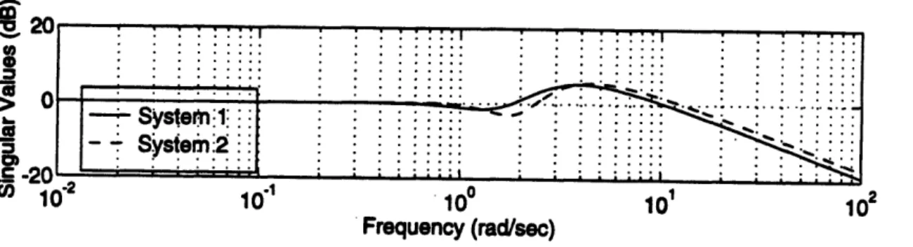
Frequency Response

The first frequency response comparison is the complementary

sensitivity of the closed-loop systems, shown in Figure 5.3. The plot indicates that the bandwidth for the LQR design is approximately 10

radians/sec,

50 M ra 'O0 0 CO) C -50

and for the frequency weighted

H. design, 20

System 1 102 Frequency (rad/sec) System 2 102 Frequency (rad/sec)

Complementary Sensitivity Comparison

5.2

u...

:. ;;;

...

... '. " -,;

...

. ' : ' ;...

... ;

.

·· ''.

...

' · ' : ' ; '

.

. ...

. ...

' ; ' ;':'...

.

... ... ...

.

;

... . ...

..·"...':'.'....

..

:.

...

·

"~

_{~ ~~~~~~~~ ~ ~~~~~~~~ ~ ~~~~~~~~~~~~~~~~~~~'}

';' "

';';':~

' ' '

. ... ,. ,.;'.-... ... .,... ... ... ... ... ... · . _{. ; . ...} ;..._... ... ... ... ... ... . ... ... .::

.

...

...

. ...

. . ...

.

;

:-

: ;; ; ; ; ' ;

;.

; ; ; ; ..

;...;... . ...

..

; .

.

.~~~~ ::: :::::' _{. . .}:: : ::: _{· ·. .} · _{. .. .};_.::I _\ . .-- :::: .. t·

~i;:

~ : :: ._ .· ::::: · · . : :: . . ::::. . . ... ~~~.. _~~~. . ... _.. .. l _... A.... ~ _< . ... __ .i~gs .-_^ nii~ _{, , . . , ; ; ; ;;} . .. _, . _{; ::: 1} · _{: : : :::::~~~~~~~''} ,.0' 10'' 10o 101 lo 105 m cn uv 0 -5 103 103 .-IA' 10' 100 101 Figure 5.3 104 10l -r-1¥ I - ...- r. ....--... . .-. ...---.... . .--...-. . ...---. I I

Arn_{Y · · · ··r ' ' """I ' ' """I ' ' ' ""'I ' ' "'"I}

r ·

i

·t i ·:· · · · ·:· · ·:· :· i ·· :·:·:r · · · · i · · i · i ·:· i i i :· · · · ·:· · ·:· :· r ·· :····

.s

_,··· i· Y·i-: , ''':'':':':':::::'' ''':''':'':': ':':'::: '''':''::'' Q' '''''''' 4. . · · · )·u

radians/sec. Both designs have roll-offs of 20dB/decade, although the roll-off does not begin for the H design until about 200 radians/sec. The plot also indicates that the LQR designs can tolerate larger

multiplicative errors at the plant input.

Figures 5.4 and 5.5 show the disturbance rejection properties

for the closed-loop systems for both design methods. The plots

indicate that the frequency weighted H designs amplify the

disturbances less than the LQR designs for frequencies less than approximately 3 radians/sec, but the LQR designs have better

disturbance rejection properties at frequencies higher than this.

For

both design methods, the disturbances are better rejected when they

appear on the longer rod.

Disturbance fl

"J'

. : :: ...

_c

'.:

...

...

... ... -- weighlite H-Infinity 20 10 100 101 lo2 103 Frequency (rad/sec) Disturbance f2 ^00 101' 101 102 10 Frequency (rad/sec)

Figure 5.4 Disturbance Rejection Comparison, System I

_ ZVV -co 2

nn

--::1 ::T""r · · -r"l -· ' i "'T -·'···r····i _{''-L'''5''"''·''·' ·-· '''''··r···r-· · -.} L : : _I vv