The Dynamic Reorganization of Cortical Network Interactions during Visual Selective Attention

(1)

The Dynamic Reorganization of Cortical Network

Interactions during Visual Selective Attention

par

Mattia Federico Pagnotta

Rome, Italie

Semestre de printemps 2020

Thèse cumulative de Doctorat

Présentée à la Faculté des lettres et des sciences humaines

de l’Université de Fribourg (Suisse)

Pour obtenir le titre de Docteur ès sciences en psychologie

Approuvé par la Faculté des lettres et des sciences humaines sur proposition des Professeurs

Gijs Plomp (première rapporteur), Björn Rasch (deuxième rapporteur), et Laura Astolfi

(troisième rapporteure). Fribourg, le 25 mai 2020. La Doyenne Prof. Bernadette Charlier

Pasquier.

(2)

(3)

i

Summary

Visual selective attention prioritizes the processing of behaviorally relevant over irrelevant information, to optimize the use of limited cognitive resources in the brain. These selective mechanisms preferentially route relevant neuronal representations through a network of distributed brain regions. Previous studies suggested that selective information routing in the attention network may be mediated by brain activity modulations in the alpha (α, 7–14 Hz) and beta-band (β, 15–30 Hz). However, the precise temporal dynamics of the cortical network interactions that support selective attention remain unclear. The investigation of these dynamic network interactions, given their fast and flexible nature, requires time-varying connectivity methods that can correctly estimate rapidly changing patterns of large-scale directed interactions between brain regions. While several such methods have been proposed, there is a lack of unbiased and systematic assessments of their performance and estimation accuracy.

The objective of this thesis was twofold: first, to critically assess and compare the performance and estimation accuracy of time-varying directed connectivity methods; second, to provide a comprehensive characterization of the dynamic reorganization of cortical network interactions during visual selective attention, under different task demands.

To systematically compare currently available time-varying directed connectivity methods, I used a combination of numerical simulations and real benchmark data recorded from rats during unilateral whisker stimulations. I showed advantages and shortcomings of the two main classes of methods, which rely on either multivariate autoregressive modeling or spectral decomposition of the recorded signals. The results served as starting point to develop innovative methods with improved performance and estimation accuracy.

I employed these novel methods together with electroencephalography (EEG) source-imaging, to investigate how cortical network interactions mediate selective attention dynamically, while healthy participants discriminated the perceived motion or orientation direction of briefly presented stimuli. The results characterized the temporal dynamics of selective attention, unveiling how attention involves both local and network changes in different frequency bands, and how these modulations further depend on the specific task demands. The results provided first evidence of the role of task-specific coupling mechanisms in supporting the selective anticipation and processing of task-relevant stimuli, through different low-frequency carriers in the β and α-band, respectively. These findings integrated into a dynamical framework existing theories of how brain rhythms establish inter-areal communication and local computation in the attention network.

(4)

(5)

iii

Acknowledgements

First of all, my special thanks goes to Gijs Plomp, who gave me the opportunity to do a Ph.D. in his research group at the University of Fribourg, providing tremendous supervision and support throughout these last four years.

I would like to express my sincere gratitude to my colleagues David Pascucci and Giovanni Mancuso, for the stimulating discussions, their helpful comments and suggestions, and for their friendship outside work. I am also grateful to all my other colleagues: Ivan Larderet, Laura Cohen, Joan Rue Queralt, and Elham Barzegaran.

I would like to thank Mukesh Dhamala (Georgia State University, USA), for the great collaboration we have had in the past years.

My sincere gratitude goes to Michaël Mouthon (University of Fribourg, CH) who provided outstanding support to set up the MRI protocol, and to the MRI Technicians at the HFR Fribourg – Hôpital cantonal, Fabien Matthey, Eric Dafflon and Marie-Paule Oberson, who assisted me during the acquisition of MRI data.

I would also like to thank all the subjects that participated in our studies and the students who helped me with part of the data collection, Fabiola Leite Frenkle (University of Fribourg, CH) and Enrique Cifuentes Cassalett (Heidelberg University, DE).

All the studies included in this thesis were supported by the Swiss National Science Foundation grants to GP (PP00P1_157420, PP00P1_183714).

(6)

(7)

v

List of figures

2. Adaptive algorithms for directed connectivity analysis

Figure 2.1. Simulated networks and time courses of the causal influences imposed

Figure 2.2. Benchmark EEG data: recording setup and network of expected functional connections Figure 2.3. Simulation 1 on the effects of varying adaptation coefficients

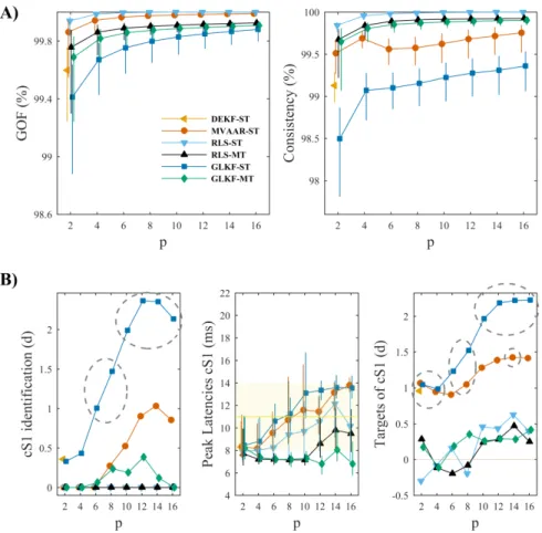
Figure 2.4. Simulation 2 on the effects of model order selection

Figure 2.5. Simulation 3 on the effects of varying sampling rate: model quality

Figure 2.6. Simulation 3 on the effects of varying sampling rate: connectivity estimation Figure 2.7. Effects of varying adaptation coefficients in benchmark EEG data

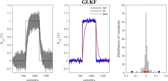
Figure 2.8. Effects of model order selection in benchmark EEG data Figure 2.9. Effects of varying sampling rate in benchmark EEG data Figure 2.S1. The two strategies for multiple realizations in GLKF Figure 2.S2. Simulation 4 on the effects of varying amount of trials

Figure 2.S3. Simulation 5 on the effects of varying sampling rate & model order: model fitting

Figure 2.S4. Simulation 5 on the effects of varying sampling rate & model order: connectivity estimation

3. The regularized and smoothed General Linear Kalman Filter

Figure 3.1. Variance of estimated AR coefficients Figure 3.2. Performance metrics

4. Nonparametric Granger–Geweke causality: methods comparison

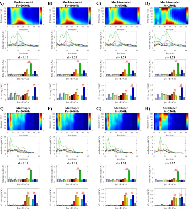
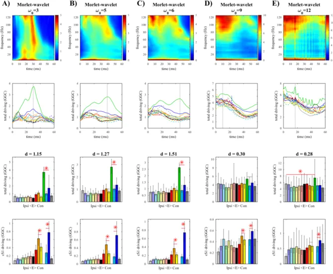
Figure 4.1. Whisker-evoked SEPs Figure 4.2. The effect of downsampling Figure 4.3. Morlet wavelet

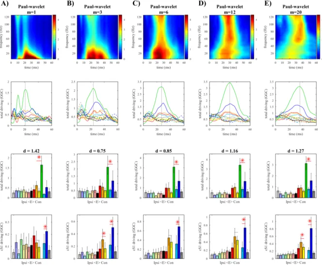
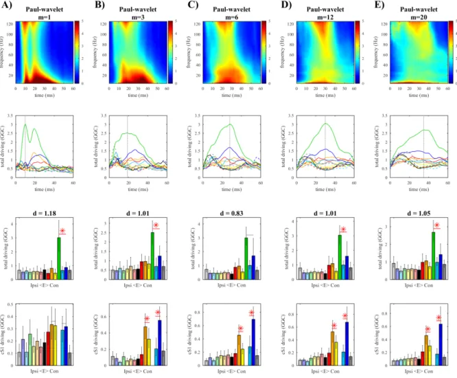
Figure 4.4. Paul wavelet

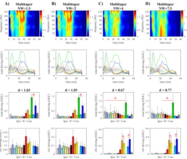
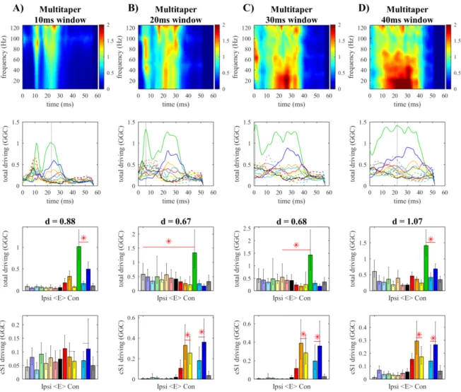
Figure 4.5. Time-bandwidth product in the multitaper Figure 4.6. Window size in the multitaper

Figure 4.7. Pairwise GGC

Figure 4.S1. The effect of downsampling (NO-TRT) Figure 4.S2. Morlet wavelet (NO-TRT)

Figure 4.S3. Paul wavelet (NO-TRT)

Figure 4.S4. Time-bandwidth product in multitaper (NO-TRT) Figure 4.S5. Window size in multitaper (NO-TRT)

(10)

viii

5. Nonparametric Granger–Geweke causality: benchmark dataset and simulation

framework

Figure 5.1. Common reference problem: uncorrelated white noise Figure 5.2. Common reference problem: same oscillatory component

Figure 5.3. Common reference problem: oscillatory component at lower frequency Figure 5.4. Common reference problem: oscillatory component at higher frequency Figure 5.5. SNR imbalance between channels (bivariate case)

Figure 5.6. SNR imbalance between channels (trivariate case): additive noise on driver Figure 5.7. SNR imbalance between channels (trivariate case): pairwise measures Figure 5.8. SNR imbalance between channels (trivariate case): conditional measures Figure 5.9. Independent white noise

Figure 5.10. Mixed white noise

Figure 5.11. Mixed white and pink noise Figure 5.12. Stokes & Purdon’s example

6. Dynamic mechanisms of attentional selection

Figure 6.1. Experimental paradigm and VEPs results

Figure 6.2. Attentional modulation of brain rhythms: comparison between Attend-motion and Unattended Figure 6.3. fMRI results and ROIs

Figure 6.4. Anticipatory differences in network efficiency

Figure 6.5. Anticipatory differences in local PAC and correlation with local network changes Figure 6.6. Stimulus-evoked differences in local α-γ PAC

Figure 6.7. Stimulus-evoked differences in network efficiency

Figure 6.8. Temporal sequence of the effects induced by visual selective attention

Figure 6.S1. Attentional modulation of brain rhythms: comparison between Attend-orientation and Unattended

Figure 6.S2. Anticipatory differences in local PAC: control analysis based on stratification Figure 6.S3. Stimulus-evoked differences in network efficiency

(11)

ix

List of tables

2. Adaptive algorithms for directed connectivity analysis

Table 2.S1. Results of the preprocessing procedures to remove bad trials Table 2.S2. DEKF-AA: invalid results in benchmark EEG varying model order

4. Nonparametric Granger–Geweke causality: methods comparison

Table 4.1. The effect of downsampling (criterion II) Table 4.2. The effect of downsampling (criterion III) Table 4.3. Morlet wavelet (criterion II)

Table 4.4. Morlet wavelet (criterion III) Table 4.5. Paul wavelet (criterion II) Table 4.6. Paul wavelet (criterion III)

Table 4.7. Time-bandwidth product in the multitaper (criterion II) Table 4.8. Time-bandwidth product in the multitaper (criterion III) Table 4.9. Window size in the multitaper (criterion II)

Table 4.10. Window size in the multitaper (criterion III) Table 4.11. Pairwise GGC (criterion II)

Table 4.12. Pairwise GGC (criterion III)

Table 4.S1. The effect of downsampling (NO-TRT, criterion II) Table 4.S2. The effect of downsampling (NO-TRT, criterion III) Table 4.S3. Morlet wavelet (NO-TRT, criterion II)

Table 4.S4. Morlet wavelet (NO-TRT, criterion III) Table 4.S5. Paul wavelet (NO-TRT, criterion II) Table 4.S6. Paul wavelet (NO-TRT, criterion III)

Table 4.S7. Time-bandwidth product in multitaper (NO-TRT, criterion II) Table 4.S8. Time-bandwidth product in multitaper (NO-TRT, criterion III) Table 4.S9. Window size in multitaper (NO-TRT, criterion II)

Table 4.S10. Window size in multitaper (NO-TRT, criterion III) Table 4.S11. Pairwise GGC (NO-TRT, criterion II)

Table 4.S12. Pairwise GGC (NO-TRT, criterion III)

6. Dynamic mechanisms of attentional selection

Table 6.1. VEPs analysis; results of repeated measures ANOVA and post-hoc tests Table 6.2. Details about the twenty-two regions of interest (ROIs)

(12)

x

List of abbreviations

cS1 contralateral primary sensory cortex CSF cerebrospinal fluid

CTC communication through coherence DEKF Dual Extended Kalman Filter EEG electroencephalography

ERD event-related desynchronization fMRI functional magnetic resonance imaging FWHM full width at half maximum

GBI gating by inhibition GC Granger causality

GGC Granger–Geweke causality GLKF General Linear Kalman Filter GLM general linear model

HRF hemodynamic response function ICA independent component analysis LFP local field potential

MEG magnetoencephalography

MNI Montreal Neurological Institute and Hospital MRI magnetic resonance imaging

MVAR multivariate autoregressive

NO-TRT without using time reversal testing (TRT) RLS Recursive Least Squares algorithm ROIs regions of interest

SEPs somatosensory evoked potentials STOK Self-Tuning Optimized Kalman filter tv-MVAR time-varying MVAR

VEPs visual-evoked potentials WGC Wiener–Granger causality WM white matter

(13)

1

1. General introduction

Attention is one of the elements of cognitive control in the brain, it is the ability to selectively direct our limited cognitive resources at the focus of our goal. When we talk about visual selective attention, we refer collectively to mechanisms that support the preferential processing of relevant stimuli over irrelevant ones (Carrasco, 2011; Scolari et al., 2014). Several aspects of these selective mechanisms remain poorly understood, among them we can identify two major unanswered questions: 1) How do brain-wide functional network interactions support selective attention? 2) What are exactly the temporal dynamics of this large-scale brain network? The main goal of this thesis was to answer these questions.

1.1. Visual selective attention

Visual selective attention can operate on the basis of spatial information and locations, or non-spatial information such as low-level visual features (e.g., motion, orientation, or color) and object-based representations (e.g., faces or houses) (Buschman & Kastner, 2015; Carrasco, 2011; Scolari et al., 2014). These selective mechanisms are associated with changes in local brain activity over distributed brain areas, modulations in the network of inter-areal interactions among these areas, and fast temporal dynamics. However, because these different aspects and effects of selective attention have been often investigated separately, their roles and possible interplay remain unclear.

Behavioral, neuroimaging and electrophysiological studies support the notion that visual stimuli compete for limited resources (for reviews see Beck & Kastner, 2009; Desimone & Duncan, 1995; Reynolds & Chelazzi, 2004). Experimental paradigms in which visual stimuli were peripherally presented at different locations of the visual field, while participants maintained fixation, were used to test this notion of neural competition. Results obtained using fMRI showed that when the stimuli are presented simultaneously the evoked responses are weaker than when the stimuli are presented sequentially, and these response differences increase in visual cortex from striate to extrastriate areas, suggesting that the allocation of resources may be resolved by specific patterns of activations in visual cortex (Beck & Kastner, 2005, 2007; Kastner et al., 1998, 2001). Other fMRI studies investigated the effects on neural processing of focusing attention to one attribute of a visual stimulus. O’Craven and colleagues, for example, employed visual stimuli with both moving and stationary dots, and found that the activation in motion-processing area MT–MST (V5) was significantly higher when the moving dots were attended, compared to when the stationary dots were attended (O’Craven et al., 1997). These findings suggested that local neural activity in occipital areas is selectively modulated by attention,

(14)

2

and that paying attention to stimulus features enhances neural activity in the cortical areas specialized to process those features. Selective attention may thus be supported by specific patterns of activations over functionally-specialized areas in visual cortex.

Several studies showed attentional effects on the event-related potentials (ERPs) obtained using electroencephalography (EEG) and magnetoencephalography (MEG) (Daffner et al., 2012; Hillyard & Anllo-Vento, 1998; Schoenfeld et al., 2007), and suggested that attention may be supported by precise temporal sequences of task-specific local activations (Schoenfeld et al., 2014). In particular, attention has been shown to modulate early ERP components like the P1 (or P100, within 100 ms of stimulus onset). Zhang and Luck showed for example that color-based attention modulates feedforward visual processing, as reflected by the P1 component, even for visual stimuli presented at unattended spatial locations (Zhang & Luck, 2009). Notably, ERPs studies extended the fMRI results by revealing the highly dynamic nature of selective attention. Neuroimaging studies have further shown that the attentional modulations of local rhythmic activity are characterized by dynamic effects in different frequency bands. Stimulus-induced decrease in power in the alpha (α, 7–14 Hz) and beta-band (β, 15– 30 Hz), also known as event-related desynchronization (ERD), has been shown to be stronger for attended stimuli than ignored ones, especially over the fronto-parietal cortex (Mazaheri & Picton, 2005; Pascucci et al., 2018). While all these findings revealed selective attentional modulations of local activity in distributed brain areas, selective attention may furthermore be mediated by specific functional connections between these areas.

Cortical network interactions among distributed brain areas are thought to control the local attentional modulations of neural activity, and a more network-centric perspective of selective attention has emerged over the years (Corbetta & Shulman, 2002; Greenberg et al., 2010; Kastner & Ungerleider, 2000; Serences & Yantis, 2007). There has been increasing effort to characterize the brain rhythms that mediate attention, by enhancing selectively relevant neuronal representations and routing them preferentially through a large-scale network in the brain (Buschman & Kastner, 2015). Different brain rhythms may provide the building-blocks of mechanisms that enable flexible control, in both attention and other cognition functions, and support the ability to adaptively (re)direct our cognitive resources, depending on behavioral goals, task demands, and context (Antzoulatos & Miller, 2014, 2016; Bonnefond & Jensen, 2015; Buschman et al., 2012; Haegens, Handel, et al., 2011; Spitzer & Haegens, 2017).

To understand how cortical network interactions support selective attention, thus requires a better understanding of what the possible different roles of distinct brain rhythms are, and how these rhythms underlie the flexible control of cortical network interactions during selective attention.

(15)

3

1.2. Brain rhythms for selective attention

Since Berger described human EEG patterns with rhythmic activity in the frequency range 8–12 Hz (α-band) (Berger, 1929), different brain oscillations have been observed at different frequencies using EEG, MEG and local field potential (LFP) (Buzsáki, 2006; Buzsáki et al., 2012). The ubiquitous nature of neuronal oscillations across spatial scales in the brain suggests that they may be functionally relevant for the synchronization of local and large-scale brain networks (Buzsáki & Draguhn, 2004), which is thought to establish inter-areal communication and selective information routing in cognitive networks (Fries, 2005, 2015; Jensen & Mazaheri, 2010).

Several studies have investigated how brain rhythms may impact large-scale communication and local computation in the brain, suggesting distinct roles for the rhythms at low frequencies and those at high frequencies (Buzsáki & Draguhn, 2004; Canolty et al., 2007; Kopell et al., 2000; von Stein & Sarnthein, 2000). These studies have shown that different brain rhythms not only provide different temporal windows of efficient inter-areal communication and processing, but they are also associated with distinct spatial scales. Low-frequency oscillations are able to synchronize over longer conduction delays and thus mediate long-range inter-areal interactions. High-frequency activity, on the other hand, is typically associated with more local neuronal computations. The interactions between oscillations at different frequencies, named cross-frequency coupling, may provide the mechanism to integrate activity from low and high frequencies, and aid large-scale network synchronization for specific cognitive functions (Buzsáki, 2006; Canolty et al., 2006; Canolty & Knight, 2010; Jensen & Colgin, 2007).

In connection with these previous findings, two main theories emerged that proposed how synchronization between neuronal oscillations may establish inter-areal communication and selective routing of information: gating by inhibition (GBI) and communication through coherence (CTC). The GBI theory proposed that oscillatory activity in the α-band reflects pulsed inhibition and plays a central role in allocating resource and routing information to task-relevant regions, by functionally closing or gating task-irrelevant connections paths (Jensen & Mazaheri, 2010). Based on the observation that increases in gamma-band activity (γ, above 30 Hz) typically co-occur with a decrease in the α-band, the GBI theory further suggested that γ-band activity reflects neuronal processing and is bound to be implicated in neuronal communication. Differently, the CTC theory proposed that inter-areal communication emerges from a flexible γ-band coherence pattern (Fries, 2005). According to this second theory, the phase synchrony between two brain areas is established in the γ-band, with neuronal oscillations in one area entraining oscillations in the other area, and this flexibly increases the functional connection between the two areas, providing selective information routing.

(16)

4

The two theories started to converge throughout the years, and a new version of CTC put more emphasis on low-frequency rhythms, proposing a role for α and β rhythms in mediating top-down influences (Fries, 2015). More recently, a framework was introduced to unify the two theories, proposing that flexible inter-areal communication is based on nested oscillations (Bonnefond et al., 2017). This unified framework suggested that the synchronization of slow oscillations in the theta (θ, 3–7 Hz), α or β-band supports inter-areal communication and information flow, while fast oscillations in the γ-band are locally nested within slow oscillations, such that the cross-frequency coupling of slow and fast oscillations temporally coordinates the information routing of γ-band activity, related to local neuronal computations.

Leveraging this concept of nesting among oscillations, a recent study introduced a “rhythmic theory of attention” (Fiebelkorn & Kastner, 2019). This theory proposed that spatially-directed attention is shaped over time by a specific organization of brain rhythms, with distinct roles in different frequency bands: coordination between sensory and motor functions (θ-band), sensory suppression (α-band), suppression of attentional shifts (β-band), and sensory enhancement (γ-band). According to this theory, activity in the θ-band rhythmically samples the visual environment, even in the absence of external rhythms and despite maintaining task demands, by providing a rhythmic alternation in time of two attentional states, which are respectively associated with enhanced or reduced perceptual sensitivity. The first state, characterized by increased activity in both β and γ-band, is associated with better visual-target detection, and it is thought to reflect attention-related sampling at the currently attended location. The second state, characterized by increased α-band activity, is associated with worse behavioral performance, and it is considered a window of opportunity for disengaging from the attended location and shifting to another.

It remains unclear whether this organization of brain rhythms generalizes to the attentional selection of low-level visual features or whole-object representations, and, if so, to what extent. How exactly these rhythmic mechanisms could support selective attention is actively debated. Recent studies proposed that activity in the α and β-band mediate large-scale network information routing, with different roles across the two frequency bands. On the one side, the activity in the α-band has been associated with inhibitory gating of irrelevant stimuli representations (Bonnefond & Jensen, 2015; Haegens, Nácher, et al., 2011; Jensen & Mazaheri, 2010; Mathewson et al., 2011; Mazaheri & Jensen, 2010). On the other side, the activity in the β-band has been associated to mechanisms that support the communication of relevant stimuli representations, through the formation of rule-specific neuronal ensembles (Antzoulatos & Miller, 2014, 2016; Buschman et al., 2012; Spitzer & Haegens, 2017). The interplay between these mechanisms of information routing and gating of relevant and irrelevant stimuli representations remains unclear, and so do several other aspects of selective

(17)

5

attention, such as the possible links between large-scale network activity and local cortical modulations.

Another elusive aspect of selective attention is related to its temporal dynamics. Some previous studies investigated the role of brain rhythms in providing anticipatory biasing signals, e.g., (Foxe & Snyder, 2011; Snyder & Foxe, 2010), while others investigated the time course of stimulus-evoked attentional effects, by simply characterizing ERP amplitude changes and latencies (Daffner et al., 2012; Schoenfeld et al., 2007, 2014). A comprehensive characterization of the temporal dynamics of selective attention and an explanation of the possible relationships between preparatory and stimulus-evoked effects are, however, still missing.

Therefore, the following questions remain unanswered: Do large-scale functional interactions among cortical areas operate at specific frequencies during selective attention? Is there a relationship between large-scale cortical network interactions and local cortical modulations? How do cortical network interactions change over time to mediate attentional selection? Does any association exist between anticipatory biasing signals and stimulus-evoked effects of selective attention?

In this thesis, I aimed to respond to each of these questions, addressing the (still) elusive aspects of selective attention. My goal was to provide a more comprehensive characterization of the associations that may exist between large-scale communication and local computations, and between anticipatory and stimulus-evoked attentional effects, in order to understand how the allocation of limited cognitive resources is orchestrated in our brain, depending on different task demands.

This main goal of the experimental project required to address some methodological challenges. In particular, the quest for correctly characterizing large-scale networks with functional connections changing rapidly over time required methods that can reliably track their (possibly fast) dynamics. These methods are described more in details in the next section.

1.3. Dynamic functional connectivity

Attention and other cognitive processes in our brain are supported by large-scale networks of dynamic interactions (Behrens & Sporns, 2012; Bressler, 1995; Horwitz, 2003; Sporns, 2010, 2014; Varela et al., 2001b). Interactions between brain areas are inherently directed, reflecting how the activity in one cortical area drives the activity in other areas through synaptic projections (Felleman & Van Essen, 1991; Markov et al., 2014). To be effective, these functional connections among brain areas change quickly over time, on subsecond time scales (Bullier, 2001; Hupé et al., 2001; Nowak & Bullier, 1997; Quinn et al., 2018). To understand how selective attention is mediated by these large-scale networks, it is then crucial to accurately characterize the underlying patterns of inter-areal connections and how these unfold over time.

(18)

6

Functional connections among cortical areas are defined as statistical regularities between the signals simultaneously recorded from them. Directed functional connectivity can be estimated by employing measures based on the concept of Granger causality (GC). GC analyses come from a long tradition that began with the notion of causality introduced by Wiener (Wiener, 1956), and continued with the statistical definitions proposed in the time domain (Granger, 1969) and frequency domain (Geweke, 1982, 1984). The temporal and spectral variants of GC are here referred to as Wiener– Granger Causality (WGC) and Granger–Geweke Causality (GGC), respectively. Measures closely related to GGC have been defined on the basis of spectral quantities obtained from a multivariate autoregressive (MVAR) model of the time series. In the MVAR model, the signals simultaneously recorded from different brain areas are modeled through a system of linear equations where each variable (brain area) has an equation that explains the evolution of its signal, on the basis of past samples (weighted) of its own and of the other variables, and an error term (random noise). The model order determines the number of past observations included in the model, while the coefficients matrix contains the weights in the model (see also Chapter 2). Spectral measures related to GGC can be derived from Fourier-transformed coefficients matrix, or its inverse (spectral transfer matrix), eventually scaled by the noise (Astolfi et al., 2006, 2007; Baccalá & Sameshima, 2001, 2014; Kaminski & Blinowska, 1991; Takahashi et al., 2010; Toppi et al., 2013).

In general, analyses based on the Granger-causal framework make use of inferences based on the notion of temporal precedence and statistical predictability among simultaneously recorded neural time series. These techniques are data-driven and do not require priors, for this reason they are often referred to as exploratory, in contraposition to confirmatory techniques in which an explicit generative model is specified a priori and data are successively used to assess the plausibility of the model (Bressler & Seth, 2011; Roebroeck et al., 2011). GC analyses have become popular in the field of neuroscience because they can be formulated in a multivariate framework and in the frequency-domain, which allows characterizing the brain rhythms structures that support cognitive functions. The estimation of spectral causality measures (e.g., GGC) can be derived using two distinct classes of approaches, commonly referred to as parametric and nonparametric methods. The distinction between the two classes comes from the way in which the covariance matrix and spectral transfer matrix of the linear system are estimated.

In their classical formulation, spectral GGC estimates are derived from MVAR modeling of the recorded time series, which, after Fourier transformation of the estimated matrix of model coefficients, allows estimating the spectral transfer matrix and cross-spectral density matrix of the system (Geweke, 1982, 1984). This approach requires the a priori choice of the model order, which is the parameter that determines how many past time samples are considered for predicting the activity at present time. For this reason, the MVAR-based methods are named parametric. Parametric methods have been

(19)

7

successfully used to investigate directed inter-areal interactions between visual areas (Bernasconi et al., 2000; Bernasconi & König, 1999), sensorimotor processing (Brovelli et al., 2004; Zhang et al., 2008), and cognitive tasks (Ding et al., 2006; Roebroeck et al., 2005).

Alternative methods allow deriving GGC estimates from a spectral factorization of the time series, and are referred to as nonparametric because the explicit MVAR modeling is completely bypassed (Dhamala et al., 2008a, 2008b). Nonparametric methods have also been successfully employed to investigate causal influences in visual processing and selective attention (Bastos et al., 2015; Bosman et al., 2012a; Roberts et al., 2013; Saalmann et al., 2012), information processing in auditory cortex (Fontolan et al., 2014), and to evaluate directional influences between spike trains (Cao et al., 2012; Chen et al., 2014; Nedungadi et al., 2009).

Notably, both parametric and nonparametric methods allow for implementations that enable to overcome the assumption of signal stationarity across time. This is important because it allows to estimate time-varying functional interactions among brain areas. Parametric methods can be implemented using a time-varying MVAR (tvMVAR) model of the signals, which can be computed using adaptive algorithms (Arnold et al., 1998a; Milde et al., 2010; Wilke et al., 2008). In a similar way, nonparametric methods allow also for an implementation of time-varying GGC, either by using wavelet transforms for time-varying spectral decomposition (Daubechies, 1990; Torrence & Compo, 1998), or by employing the multitaper method on a sliding time window (Thomson, 1982).

Before this thesis, while several time-varying connectivity methods were available, there was a lack of unbiased systematic comparative analyses of their performance and of their robustness against parameter changes, especially in real data applications. Hence, I aimed to provide an objective assessment of their performance by critically comparing their estimation accuracy in both simulations and real data.

1.4. Outline of the thesis

This thesis contains the findings of two main projects: one methodological and one experimental. My principal objective was to investigate how oscillatory cortical network interactions dynamically support visual selective attention. To this end, the experimental project consisted of an EEG and fMRI study on healthy human participants that varied selective attention by having participants perform different discrimination tasks on visual stimuli with identical physical properties, which were always presented at the same spatial location around a central fixation spot (Pagnotta et al., in preparation). The participants either attended or ignored the visual stimuli, depending on task demands, which allowed me to characterize how rhythmic network interactions in our brain dynamically shape selective attention.

(20)

8

I used EEG because its temporal resolution enables to investigate the temporal dynamics of selective attention in noninvasive way, and also the underlying brain rhythms modulations. A source reconstruction technique was employed to estimate and localize the EEG sources of brain electrical activity (Michel et al., 2004; Rubega et al., 2019; Van Veen et al., 1997). This approach was used since there is no one-to-one relationship between activity recorded at EEG electrodes positions and activity in cortical areas underneath, and because connectivity analyses on sensor-space do not allow interpretations in terms of interacting cortical areas (Brunner et al., 2016; Van de Steen et al., 2016), To optimize this procedure, the individual coordinates of the 3D electrodes positions were used for each participant, together with an individual participant’s whole-head anatomical image obtained using MRI. This allowed to create individual realistic head models of the different participants (Hamalainen & Sarvas, 1989; Oostenveld et al., 2011). All connectivity analyses were then performed on source-reconstructed time series.

Source-reconstructed time series were extracted from cortical regions of interest (ROIs) across the brain, which were previously identified using an fMRI experiment. In this experiment, the same participants performed the same visual discrimination tasks, but inside the MRI-scanner. Leveraging the better spatial resolution of fMRI, a statistical analysis on fMRI data was performed to reveal cluster-peaks of significant differences between attention conditions that were used to identify functionally-relevant cortical areas in the attention network, serving for the definition of the ROIs for EEG source-reconstruction and successive analyses.

As previously mentioned, my aim was not only to characterize the functional cortical network interactions that support selective attention, but also to reveal how these large-scale interactions dynamically change and reorganize during selective attention. I needed a time-varying connectivity method able to reliably estimate the temporal dynamics of rapidly changing patterns of such functional interactions. For this reason, I conducted methodological studies that consisted of a systematic validation and comparison of methods to derive measures of dynamic directed functional connectivity, both parametric and nonparametric, that are currently available.

In two studies (Pagnotta et al., 2018b; Pagnotta & Plomp, 2018), the performance of time-varying directed connectivity methods were systematically compared using numerical simulations and benchmark somatosensory data, previously recorded during unilateral whisker stimulations in rats (Plomp, Quairiaux, Michel, et al., 2014; Quairiaux et al., 2011). The findings of these studies led to the development of a freely available toolbox (nonparametricGGC_toolbox) that allows computing GGC with different nonparametric methods and a simulation framework for the assessment of their pitfalls (Pagnotta et al., 2018a).

Since the results proved that the General Linear Kalman Filter (GLKF) is the most accurate and reliable among the existing parametric algorithms (Pagnotta & Plomp, 2018), I started from the

(21)

9

original implementation of GLKF to develop an improved version of the algorithm, by incorporating

ℓ1 norm penalties to promote sparse solutions and a smoothing procedure to increase the robustness of

the estimates (Pagnotta et al., 2019). This novel method was named the sparse and smoothed General Linear Kalman Filter (spsm-GLKF).

Following the General introduction (Chapter 1), the contributions of this cumulative thesis are presented as follows:

• Chapter 2 contains the findings of the comparative study on parametric methods for dynamic functional connectivity (Pagnotta & Plomp, 2018).

• Chapter 3 describes the novel parametric method spsm-GLKF (Pagnotta et al., 2019).

• Chapter 4 provides the findings from the systematic assessment of the performance of existing nonparametric methods (Pagnotta et al., 2018b).

• Chapter 5 presents the nonparametricGGC_toolbox and simulation framework (Pagnotta et al., 2018a).

• Chapter 6 illustrates the findings of the EEG and fMRI study on visual selective attention (Pagnotta et al., in preparation).

• Chapter 7 presents concluding remarks, along with an outline of the limitations and potential future work.

1.5. Publications

Four Chapters (2–5) of this thesis have been published as articles in peer-reviewed scientific journals and peer-reviewed conference proceedings. Chapter 6 is currently in preparation and will be submitted for peer-review soon. A detailed list of these publications is provided below.

Publications in peer-reviewed scientific journals:

Pagnotta, M. F., & Plomp, G. (2018). Time-varying MVAR algorithms for directed connectivity analysis: Critical comparison in simulations and benchmark EEG data. PloS

one, 13(6), e0198846. https://doi.org/10.1371/journal.pone.0198846

Pagnotta, M. F., Dhamala, M., & Plomp, G. (2018). Benchmarking nonparametric Granger causality: Robustness against downsampling and influence of spectral decomposition parameters. NeuroImage, 183, 478-494. https://doi.org/10.1016/j.neuroimage.2018.07.046

(22)

10

Pagnotta, M. F., Dhamala, M., & Plomp, G. (2018). Assessing the performance of Granger– Geweke causality: Benchmark dataset and simulation framework. Data in brief, 21, 833-851. https://doi.org/10.1016/j.dib.2018.10.034

Peer-reviewed conference proceedings:

Pagnotta, M. F., Plomp, G., & Pascucci, D. (2019). A regularized and smoothed General Linear Kalman Filter for more accurate estimation of time-varying directed connectivity. In 2019 41st Annual International Conference of the IEEE Engineering in Medicine and

Biology Society (EMBC). IEEE. https://doi.org/10.1109/EMBC.2019.8857915

In preparation:

Pagnotta, M. F., Pascucci, D., & Plomp, G. (in preparation). A rapid sequence of network and oscillatory mechanisms mediates visual selective attention.

(23)

11

2. Adaptive algorithms for directed connectivity analysis

1

Brief summary

In this study, we systematically compared the performance of adaptive algorithms for tvMVAR modeling, which provide a parametric approach to estimate dynamic interactions from physiological signals and derive measures of directed functional connectivity (Milde et al., 2010; Möller et al., 2001; Omidvarnia et al., 2011; Schlögl, 2000). The physiological plausibility of the results obtained with these parametric methods was assessed using both numerical simulations and benchmark somatosensory evoked potentials (SEPs), which were previously obtained from Wistar rats during unilateral whisker stimulations (Plomp, Quairiaux, Michel, et al., 2014; Quairiaux et al., 2011). Our findings identify strengths and weaknesses of existing tvMVAR approaches and provide practical recommendations for their application in real data.

1_{Published as: Pagnotta, M. F., & Plomp, G. (2018). Time-varying MVAR algorithms for directed connectivity}

analysis: Critical comparison in simulations and benchmark EEG data. PloS one, 13(6), e0198846. https://doi.org/10.1371/journal.pone.0198846

(24)

12

Abstract

Human brain function depends on directed interactions between multiple areas that evolve in the subsecond range. Time-varying multivariate autoregressive (tvMVAR) modeling has been proposed as a way to help quantify directed functional connectivity strengths with high temporal resolution. While several tvMVAR approaches are currently available, there is a lack of unbiased systematic comparative analyses of their performance and of their sensitivity to parameter choices. Here, we critically compare four recursive tvMVAR algorithms and assess their performance while systematically varying adaptation coefficients, model order, and signal sampling rate. We also compared two ways of exploiting repeated observations: single-trial modeling followed by averaging, and multi-trial modeling where one tvMVAR model is fitted across all trials. Results from numerical simulations and from benchmark EEG recordings showed that: i) across a broad range of model orders all algorithms correctly reproduced patterns of interactions; ii) signal downsampling degraded connectivity estimation accuracy for most algorithms, although in some cases downsampling was shown to reduce variability in the estimates by lowering the number of parameters in the model; iii) single-trial modeling followed by averaging showed optimal performance with larger adaptation coefficients than previously suggested, and showed slower adaptation speeds than multi-trial modeling. Overall, our findings identify strengths and weaknesses of existing tvMVAR approaches and provide practical recommendations for their application to modeling dynamic directed interactions from electrophysiological signals.

(25)

13

2.1. Introduction

All sensory and cognitive processes, including resting state activity, arise from the coordinated activity of multiple brain areas (Bressler, 1995; Felleman & Van Essen, 1991; Mantini et al., 2007; Sporns, 2014; Varela et al., 2001a). Brain areas continuously coordinate their activity through directed interactions, with activity in one area driving the activity in other areas through direct synaptic projections. To be useful, these inter-areal interactions must happen on small time scales, of the order of tens of milliseconds (Brodbeck et al., 2012; Nowak & Bullier, 1997). A better characterization of how directed network interactions evolve over time and under varying experimental conditions is crucial for understanding the functional role of single areas, as well for determining periods of network stability and change (Deco et al., 2011; Fairhall & Ishai, 2007; Liang et al., 2017; Vidaurre et al., 2016, 2017). An important challenge, therefore, is how to derive estimates of directed connectivity between brain areas from multiple simultaneously recorded neurophysiological time series, as obtained with high temporal resolution using electroencephalography (EEG), magnetoencephalography (MEG) or local field potential (LFP) recordings.

Time-varying multivariate autoregressive (tvMVAR) modeling is a parametric approach to estimate dynamic interactions from physiological signals and derive measures of directed functional connectivity (Arnold et al., 1998a; Ding et al., 2000; Wilke et al., 2008; Winterhalder et al., 2005). In this framework, algorithms based on recursive estimation were developed to provide valid models of non-stationary neural data (Milde et al., 2010; Möller et al., 2001; Omidvarnia et al., 2011; Schlögl, 2000; Sommerlade et al., 2009). Several such algorithms have been successfully used to characterize dynamic network interactions in sensory and motor processing (De Vico Fallani et al., 2008; Hu et al., 2012; Petrichella et al., 2017; Plomp, Quairiaux, Michel, et al., 2014; Plomp et al., 2016; Weiss et al., 2008), cognitive tasks (Garcia et al., 2017), and pathological activity in epileptic patients (Coito et al., 2015; van Mierlo et al., 2011; Wilke et al., 2008).

Recursive algorithms for tvMVAR modeling require the a priori choice of two parameters: the model order and the adaptation coefficient. The model order is the maximum number of lagged observations included in the model. Several information criteria can be used to select an optimal model order (Akaike, 1969, 1974; Grünwald, 2007; Hannan & Quinn, 1979; Schwarz, 1978), of which Akaike’s information criterion (AIC) and Bayesian information criterion (BIC) are most often used. Unfortunately, information criteria in practice often disagree about the optimal model order because they minimize different contributes or they may not converge to an optimal order at all (Porcaro et al., 2009); these limitations strongly motivate an evaluation of the robustness of tvMVAR methods to variations in model order.

(26)

14

The adaptation coefficients are used in recursive algorithms to regulate the adaptation speed of parameters estimation and have to be selected between zero and one (Milde et al., 2010; Möller et al., 2001). Values close to one lead to a faster adaptation (‘adaptivity’) but also a greater variance of parameter estimates, and this trade-off holds vice versa for values close to zero (Leistritz et al., 2013; Möller et al., 2003a). Thus, if the adaptation coefficients are not properly tuned, the performance of the recursive algorithm may be significantly degraded.

While tvMVAR algorithms have been previously tested in simulations (Leistritz et al., 2013; Milde et al., 2010; Schlögl, 2000; Toppi et al., 2012), a systematic investigation into their robustness against parameter changes in real data is still missing. We therefore critically compared four algorithms that are commonly used to model non-stationary neurophysiological signals: the Recursive Least Squares (RLS) algorithm (Möller et al., 2001) and three algorithms based on Kalman filter, which are the General Linear Kalman Filter (GLKF) (Milde et al., 2010), the multivariate adaptive autoregressive (MVAAR) estimator (Schlögl, 2000), and the Dual Extended Kalman Filter (DEKF) (Omidvarnia et al., 2011; Sommerlade et al., 2009).

When multi-trial time series are available, information from single trials can be combined in tvMVAR models to improve estimation accuracy and reliability of connectivity estimates (Möller et al., 2003a). Two strategies can be adopted to make use of multiple realizations: i) single-trial tvMVAR modeling followed by averaging across trials (Mullen, 2014; Omidvarnia et al., 2014); ii) multi-trial modeling, in which one tvMVAR model is simultaneously fitted to all trials (Milde et al., 2010; Möller et al., 2001, 2003a). The relative advantages of each approach and their sensitivities to parameter settings have not been systematically tested, but are important to understand when using these techniques in real data.

Here we provide a critical and comprehensive evaluation of the four recursive algorithms for tvMVAR modeling and the two ways of exploiting multiple realizations. To do so, we first used well-controlled simulated data and then exploited real benchmark EEG recordings that were previously obtained from rats in a somatosensory experiment where the ground truth is known (Plomp, Quairiaux, Michel, et al., 2014; Quairiaux et al., 2011). In simulations and real data we measured both model quality and the accuracy of the estimated connectivity strengths and dynamics, while varying adaptation coefficients, model order, and sampling rate. We included variations in sampling rate because downsampling is commonly used in M/EEG and LFP analyses, but how this procedure affects the estimation accuracy of tvMVAR algorithms using these data is not well understood yet.

(27)

15

2.2. Methods

2.2.1. Time-varying MVAR models

The general form of a d-dimensional tvMVAR process of order p can be expressed as:

𝑌 𝑛 = 𝐴! 𝑛 𝑌 𝑛 − 𝑟 + 𝐸(𝑛) !

!!!

(2.1)

For each time step n=1,2,…N the MVAR coefficients matrix Ar(n)∈Rdxd and E(n) is a zero-mean

uncorrelated d-dimensional white noise vector process.

We considered four recursive algorithms to estimate tvMVAR models. The first was the Recursive Least Squares (RLS) algorithm (Möller et al., 2001), which extends the Yule–Walker equations for the estimation of MVAR processes to the nonstationary case. For the adaptive estimation of the MVAR coefficients matrix RLS uses a forgetting factor λ that weights the error function stepwise in time and has to be selected a priori between 0 and 1. The algorithm initializes the update term C as a dp-by-dp matrix of zeros. Then the recursive estimation at each step is obtained by repeating the following computations for n=p+1,…,N:

𝑋_!= 𝑥_!!!, … , 𝑥_!!! 𝐶!= 1 − 𝜆 𝐶!!!+ 𝑋!!𝑋! 𝐾_! = 𝑋_!𝐶_!!! 𝑍_! = 𝑥_!− 𝑋_!𝐴(𝑛 − 1)! 𝐴 𝑛 = 𝐴 𝑛 − 1 + 𝑍!!𝐾! (2.2)

with X being the observations on the previous p lags, K the gain matrix, Z the innovation matrix, and A the matrix of the MVAR coefficients of dimension d-by-dp. In this recursive estimation, the gain matrix gives more weight to measures with lower variance. The innovation is computed as the difference between observed and expected data and used to update the MVAR coefficients matrix.

The other algorithms here considered are based on the Kalman filter. The General Linear Kalman Filter (GLKF) algorithm (Arnold et al., 1998b; Milde et al., 2010) is one of them and is defined by two equations: an observation equation (2.3), which connects the state process with the observation, and a state equation (2.4), which models the state process as a random walk process.

𝑂!= 𝐻!𝑄!+ 𝑊! (2.3)

(28)

16

where the index n determines the time instant at which the estimation is performed, O indicates the observations, H is the transition matrix, Q is the state process, W is an additive observation noise, G is a transition matrix of a random walk process, and V is an additive process noise. The state process is defined in terms of parameter matrix, Ar(n) from equation (2.1), as follows:

𝑄!=

𝐴_!(𝑛)! ⋮

𝐴_!(𝑛)! (2.5)

When multiple trials are available, GLKF allows for single-trial modeling as well as multi-trial modeling. In the latter approach, the expected value of the additive observation noise covariance matrix is computed at each step with a recursive equation, in which the update term is obtained from the average covariance matrices of prediction error across k trials (Milde et al., 2010; Schack et al., 1995):

𝑊_!= 𝐼_!, 𝑊_!= 𝑊_!!! 1 − 𝑐_! + 𝑐_! 𝑂_!− 𝐻_!𝑄_!!! !_(𝑂

!− 𝐻!𝑄!!!)/(𝑘 − 1) (2.6) where Id is a d-dimensional identity matrix, and the other terms come from equations (2.3) and (2.4).

The algorithm uses two adaptation constants c1 and c2 that play a role similar to the forgetting

factor in RLS, and also have to be set between zero and one. The constants c1 regulates the proportion

between estimates at the previous step and the update term in equation (2.6), while the constant c2

weights the expected value of the additive process noise covariance matrix, which is estimated constantly as a weighted identity matrix of dimension dp-by-dp, as follows:

𝑉! = 𝑐!𝐼!" (2.7)

By tuning the two adaptation constants it is possible to regulate the speed of adaptation to transitions in temporal dynamics of connectivity patterns. High values increase adaptation speed but increase also estimation variance, while, low values smooth estimates in time by reducing variance but also speed in adaptation.

A second Kalman filter algorithm is the multivariate adaptive autoregressive (MVAAR) estimator (Schlögl, 2000). In this algorithm the measurement noise covariance matrix is updated using the prediction error of the previous step (Schack et al., 1995), while estimating the covariance of the additive matrix noise of the state process using a variant proposed by Isaksson and colleagues (Isaksson et al., 1981):

𝑉! = 𝑐!!𝐼!" (2.8)

where Idp is the identity matrix of dimension dp-by-dp.

A third variant of the Kalman filter, called Extended Kalman Filter, was developed to provide efficient maximum-likelihood estimates of discrete-time nonlinear dynamical systems (Wan & Nelson,

(29)

17

2001). In the Dual Extended Kalman Filter (DEKF) (Omidvarnia et al., 2011; Sommerlade et al., 2009), which is tested here, both the states of the dynamical system and its parameters are estimated simultaneously. Similarly to GLKF and MVAAR, an update coefficient has to be set between zero and one to regulate how much estimates from the previous step are included for estimation at the current step. We here used the freely available implementation of DEKF (https://www.mathworks.com/matlabcentral/fileexchange/33850-dual-extended-kalman-filter--dekf-).

When multiple trials are available, RLS and GLKF allow for both single-trial and multi-trial modeling; while DEKF and MVAAR only allow for single-trial modeling, because the multi-trial approach is currently not implemented for them. In this study we thus critically evaluated the following algorithms: i) RLS using either single-trial modeling (RLS-ST) or multi-trial modeling (RLS-MT); ii) GLKF using either single-trial modeling ST) or multi-trial modeling (GLKF-MT); iii) DEKF using single-trial modeling (DEKF-ST); iv) MVAAR using single-trial modeling (MVAAR-ST).

The Partial Directed Coherence (PDC) (Baccalá & Sameshima, 2001) is a spectral MVAR-based connectivity measure, which is able to distinguish direct from indirect connections. To infer time-varying connectivity from the different tvMVAR models we used a squared variant of the PDC in which the information flow from j to i is normalized by the total amount of inflow to i (Astolfi et al., 2006; Baccalá & Sameshima, 2001):

𝑃𝐷𝐶!"(𝑓, 𝑡) = 𝐴!"(𝑓, 𝑡) ! 𝐴_!"(𝑓, 𝑡) ! ! !!! (2.9)

This measure has been previously well-validated and tested (Astolfi et al., 2006; Plomp, Quairiaux, Michel, et al., 2014; Plomp et al., 2015; Toppi, 2013). Unless specified otherwise, time-frequency connectivity analyses were performed up to Nyquist time-frequency.

2.2.2. Numerical simulations

We used two surrogate networks, one with 5 nodes and the other with 2 nodes, which were simulated as vector autoregressive processes with time-varying causal influences between nodes as in equation (2.1). In order to simulate measurement noise we added uncorrelated white Gaussian noise to the time series of each node in each simulated condition. The variance of these noise terms was adjusted to produce a signal-to-noise ratio of 20 dB, which is here defined as the ratio of signal variance and noise variance.

For the 5-nodes network the diagram in Figure 2.1A provides the layout of directed connections that are active at some point in time during each trial. All the other possible connections between nodes were constantly set to zero. Trials were simulated with a length of 2 seconds, considering 1000

(30)

18

time points at a sampling frequency of 500 Hz. The parameters b(n), c(n), d(n) and e(n) denote the time courses of causal influences imposed in the network (Figure 2.1B), i.e. each represents how the strength of the directed connection between a specific pair of nodes changes over time in every trial. For each imposed connection we imposed a lag in the autoregressive model. This lag represents the delay (in time samples) with which the signal of sender node enters in the prediction of the signal of receiver node. The imposed lags for b(n), c(n), d(n) and e(n) were 1 (2ms), 1 (2ms), 2 (4ms) and 3 (6ms) time points, respectively.

Figure 2.1. Simulated networks and time courses of the causal influences imposed. A) The diagram highlights the

directed connections (arrows) imposed in the 5-nodes network, which was used for Simulation 1. All remaining possible connections between nodes are imposed to be constantly equal to zero. B) Shows the time-courses of the causal influences imposed in the 5-nodes network (Simulation 1), i.e. the dynamic evolution of the strength of each directed connection imposed in the model. Color coding matches the colors of the arrows shown in A). C) The diagram shows the directed connection imposed from node 1 to node 2 (green arrow) in the 2-nodes network and its time course in Simulation 2. This influence is active for a total duration in time of 250 ms. D) Alternative time courses of the causal influence from node 1 to node 2, with varying total durations, are considered for Simulation 3, which makes use of the 2-nodes network.

The simpler 2-nodes network was used to test how well each algorithm models causal influences of varying durations. In this network, the time course of the parameter b(n) denotes the intensity of the causal influences from node 1 towards node 2 (Figure 2.1C), and different values were considered for the model order. Varying durations of causal influences from node 1 to node 2 were considered (Figure 2.1D). In the second model, we used a sampling frequency of 1000 Hz and trial duration of 1 second to generate the process. For both networks, we simulated datasets of 20 trials, and

(31)

19

repeated the generation-estimation procedure 50 times for each of the conditions considered. We performed a total of three simulations.

By using the general term ‘adaptation coefficients’ we henceforth refer to adaptation constants in Kalman filter algorithms, forgetting factor in RLS, and update coefficient in DEKF. In Simulation 1, using the 5-nodes network (Figure 2.1A-B), we varied adaptation coefficients from 0.001 to 0.7 in 18 logarithmic steps. We considered a fixed model order p=3 for tvMVAR fitting.

In Simulation 2, we used the 2-nodes network (Figure 2.1C) imposing different lags for the causal influence (4, 8, 12, 16 or 20 ms) and varied model orders (between 2 and 22 at step of 2).

In Simulation 3, we used the 2-nodes network (Figure 2.1C) and downsampled the generated time series (1000 Hz) using 10 sampling rate levels, from 1000 Hz to 100 Hz in steps of 100 Hz. A zero-phase antialiasing filter was used before downsampling to mitigate distortions due to aliasing. To take into account the fact that after downsampling the causal influence can be observed only through a decimated number of samples, we repeated the analysis using different durations of the imposed causal influence (Figure 2.1D). The causal influence from node 1 to node 2 (Figure 2.1C-D) had fixed lag of 10 ms, and model orders were chosen to match this lag at each sampling frequency. We here performed time-frequency connectivity analysis up to 50 Hz, which is the Nyquist frequency at lowest sampling rate.

We assessed performance of each algorithm in three ways: by quantifying tvMVAR model quality, by quantifying how well connectivity results reflected the simulated connectivity structure, and by assessing whether the timing of the dynamic interactions were correctly represented.

We used two measures of model quality: goodness-of-fit (GOF) and percent consistency. GOF reflects how much of the signal is explained by the model parameters (Schlögl, 2000), and is defined as [1-REV]*100, where REV is the relative error variance and is obtained as mean squared error (MSE) (Lehmann & Casella, 1998), i.e. the mean of the squares of the differences between observed values of the time series and values recreated from the MVAR coefficients, normalized by the variance of the observed signal. The percent consistency checks instead what proportion of the correlation structure in the data is accounted for by the model (Ding et al., 2000).

Since we simulated each network as a tvMVAR process, the simulated PDC values can be derived directly from the coefficients matrix used in each simulation itself, providing known time-frequency connectivity values for each edge in the network. We evaluated connectivity estimation accuracy by computing misses and false alarms as the normalized mean squared differences between the estimated PDC and the simulated PDC. Squared differences were calculated for each time-frequency point and then averaged across time points and frequencies, separately for edges with simulated connections (misses) and edges without simulated connections (false alarms). Both measures were successively normalized with respect to the mean squared simulated PDC values on

(32)

20

edges with simulated connections. For example, if we consider the simple 2-nodes model (Figure 2.1C), misses were computed on the edge from 1 to 2 and false alarms were computed on the edge from 2 to 1. The closer the measures are to zero, the better the connectivity estimation accuracy.

Furthermore, we defined a measure of peak delay as the average difference between estimated peak latency and simulated peak latency, evaluated on edges with simulated connections. Values of peak delay close to zero indicate correct estimation of the timing of the imposed dynamic causal influence.

2.2.3. Benchmark EEG data

In order to compare tvMVAR algorithms in real data we used previously recorded epicranial multichannel EEG from ten rats during unilateral whisker stimulations (Quairiaux et al., 2011), where structural pathways are relatively well known and the physiology has been intensively investigated, providing strong expectations about a specific configuration of functional connections between cortical areas. For this reason, this dataset allows for direct comparisons between algorithms according to previously proposed performance criteria (Plomp, Quairiaux, Michel, et al., 2014), detailed below.

Animal handling procedures were approved by the Office Vétérinaire Cantonal (Geneva, Switzerland) in accordance with Swiss Federal Laws. In the recording setup, while the rat was under light isoflurane anesthesia, a multielectrode grid was placed in contact with the skull of the animal (Figure 2.2A). Signals were acquired using a sampling rate of 2000 Hz and bandpass filtered online between 1 and 500 Hz. A total of 15 channels were recorded and these provided the nodes of the network for our analyses (Figure 2.2B). These data are freely available (https://doi.org/10.6084/m9.figshare.5909122.v1) and further details about the recording procedure can be found elsewhere (Plomp, Quairiaux, Michel, et al., 2014; Quairiaux et al., 2011).

We used a semi-automatic procedure to remove trials contaminated with artifacts (see Appendix 2.5.S1); the average number of remaining trials per animal was 65 (range 34-80). After preprocessing, we estimated an optimal model order p=8, which corresponds to a lag of 4 ms at original sampling rate (2000 Hz), by taking the median of the distribution across animals of optimal values from AIC (range 7-27) and BIC criteria (range 4-16). We opted for this approach to obtain one unique model order across animals that could be scaled across sampling rates and used in the two analyses where the model order was not explicitly varied.

(33)

21

Figure 2.2. Benchmark EEG data: recording setup and network of expected functional connections. A) Provides a

schematic representation of the setup for epicranial recording. The dashed arrow in red represents the unilateral whisker stimulation. B) The diagram shows the expected behavior of the cortical network’s connections at early latencies after whisker stimulation. This is characterized by dominant total driving from contralateral primary somatosensory cortex (cS1, node 12) at latencies between 8 and 14 ms after stimulation. At peak driving the preferential directions of cS1 connections are expected to be found towards contralateral parietal (node 14) and more frontal cortex (node 10). Bright colors are used for nodes on the contralateral hemisphere to stimulation, while pale colors are used for the nodes on the ipsilateral hemisphere.

As in the simulations, we assessed performance while varying adaptation coefficients, model orders and sampling rate. First, we evaluated the effect of varying adaptation coefficients, using the same range of values previously used in simulations. For this analysis we set the sampling rate to 500 Hz. This choice still guarantees good temporal resolution (2 ms) and sufficiently broad frequency range to correctly investigate whisker-evoked cortical interactions, while at the same time reducing computational time and model complexity, which can be particularly problematic for some recursive algorithm, as we will show later.

We then varied model order between 2 and 16 at step of 2, using fixed sampling rate (2000 Hz) and adaptation coefficients (0.02). Finally, to evaluate the effect of downsampling we used sampling rates of 2000, 1000 and 500 Hz, adjusting model order to match the 4 ms lag and keeping adaptation coefficients fixed. In each condition evaluated, the time-varying spectral connectivity matrices obtained with the different algorithms were averaged in the gamma-band (40-90 Hz), which is the predominant frequency over contralateral primary somatosensory cortex (cS1) (Plomp, Quairiaux, Michel, et al., 2014).

We evaluated model quality using GOF and percent consistency, and systematically compared connectivity performance according to three previously proposed criteria (Plomp, Quairiaux, Michel, et al., 2014), which are related to key characteristics expected in the functional network evoked by whisker stimulation (Figure 2.2B). Because whisker-evoked activity propagates from primary somatosensory cortex in the contralateral hemisphere (cS1; node 12 in Figure 2.2B), strong functional outflow is expected from cS1 at early latencies. The functional connections from cS1 are expected to