Publisher’s version / Version de l'éditeur:
Journal of ASTM International (JAI), 7, 1, pp. 1-12, 2010-01-01
READ THESE TERMS AND CONDITIONS CAREFULLY BEFORE USING THIS WEBSITE. https://nrc-publications.canada.ca/eng/copyright
Vous avez des questions? Nous pouvons vous aider. Pour communiquer directement avec un auteur, consultez la
première page de la revue dans laquelle son article a été publié afin de trouver ses coordonnées. Si vous n’arrivez pas à les repérer, communiquez avec nous à [email protected].
Questions? Contact the NRC Publications Archive team at
[email protected]. If you wish to email the authors directly, please see the first page of the publication for their contact information.
NRC Publications Archive
Archives des publications du CNRC
This publication could be one of several versions: author’s original, accepted manuscript or the publisher’s version. / La version de cette publication peut être l’une des suivantes : la version prépublication de l’auteur, la version acceptée du manuscrit ou la version de l’éditeur.
For the publisher’s version, please access the DOI link below./ Pour consulter la version de l’éditeur, utilisez le lien DOI ci-dessous.
https://doi.org/10.1520/JAI102067
Access and use of this website and the material on it are subject to the Terms and Conditions set forth at
Drying response of wood-frame construction: laboratory and modelling
Maref, W.; Lacasse, M. A.
https://publications-cnrc.canada.ca/fra/droits
L’accès à ce site Web et l’utilisation de son contenu sont assujettis aux conditions présentées dans le site LISEZ CES CONDITIONS ATTENTIVEMENT AVANT D’UTILISER CE SITE WEB.
NRC Publications Record / Notice d'Archives des publications de CNRC:
https://nrc-publications.canada.ca/eng/view/object/?id=aa7a58e0-1898-4c11-9743-c686d74eaee3 https://publications-cnrc.canada.ca/fra/voir/objet/?id=aa7a58e0-1898-4c11-9743-c686d74eaee3
http://www.nrc-cnrc.gc.ca/irc
Drying re sponse of w ood-fra m e c onst ruc t ion: la bora t ory a nd
m ode lling
N R C C - 5 3 2 3 1
M a r e f , W . ; L a c a s s e , M . A .
F e b r u a r y 2 0 1 0
A version of this document is published in / Une version de ce document se trouve dans:
Journal of ASTM International (JAI), 7, (1), Second Symposium on
Heat-Air-Moisture Transport: measurements and implications in buildings, Vancouver,
B.C. April 19, 2009, pp. 1-12
The material in this document is covered by the provisions of the Copyright Act, by Canadian laws, policies, regulations and international agreements. Such provisions serve to identify the information source and, in specific instances, to prohibit reproduction of materials without written permission. For more information visit http://laws.justice.gc.ca/en/showtdm/cs/C-42
Les renseignements dans ce document sont protégés par la Loi sur le droit d'auteur, par les lois, les politiques et les règlements du Canada et des accords internationaux. Ces dispositions permettent d'identifier la source de l'information et, dans certains cas, d'interdire la copie de documents sans permission écrite. Pour obtenir de plus amples renseignements : http://lois.justice.gc.ca/fr/showtdm/cs/C-42
--- 1-National Research Council Canada-Institute for Research in Construction (NRCC-IRC), 1200 Montreal Road Campus, Ottawa, ON, K1AA 0R6, Canada.
W. Maref
1and M.A. Lacasse
1Drying Response of Wood-Frame Construction: Laboratory and
Modelling
ABSTRACT: Recent research in the assessment of hygrothermal response of building enclosures focuses on both laboratory experimentation and modelling in which the results from both processes are compared. Evidently such type of studies can potentially offer useful information regarding the benchmarking of models and related methods to assess hygrothermal performance of wall assemblies. This paper reports on experimental results and the use of an advanced hygrothermal computer model called hygIRC to assess the hygrothermal response of various components in wood-frame wall assemblies when subjected to nominally steady-state environmental conditions. There was interest in obtaining information on the drying rates of wall components, in particular oriented strand board (OSB), featuring several different types of membrane in contact with OSB given that such results could provide direct evidence of the degree to which membranes may retain moisture and affect moisture migration. On this basis, the drying response of mid-scale specimens of approximately (0.8 by 1-m) and full-scale specimens (2.44 by 2.44-m) were assessed in a series of experiments undertaken in a controlled laboratory setting. The results were subsequently used to help benchmark simulation results obtained from hygIRC in which a comparison is made between experimental and simulation results.
KEYWORDS: Air transport, Building System, Drying, Envelope, Heat Transfer, Mass Transfer, Modeling, Moisture,
Wood Product.
INTRODUCTION
Simulation models can accommodate a variety of changing boundary conditions and as well, result in much faster analysis, given the recent advances in computer technology that have permitted ready access to enhanced computing performance. This in turn has brought about an increased emphasis on the use of numerical methods to solve the fundamental hygrothermal equations that form the basis for many of the mathematical models developed over the past decade. However, acceptance of results derived from simulation models is contingent upon acquiring evidence of a response comparable to that obtained from experimental work when the simulation is carried out under the same nominal environmental loads. Hence, studies that incorporate both laboratory experimentation and simulation offer possibilities to compare results and hence ‘benchmark’ the response models such as hygIRC to known conditions [1].
As part of a research program to establish the hygrothermal response of wood-frame wall assemblies to varying climate conditions, a series of drying experiments were performed in a programmable environmental chamber used for replicating specific temperature and relative humidity profiles, the range of which would be consistent with those of exterior climatic conditions [2,3]. In these experiments, bulk moisture content of the entire assembly was measured using a sophisticated weighing system, and as well, local moisture content measurements of oriented strand board (OSB) sheathing components were taken with the use of electrical resistance moisture pin pairs.
This paper reports on experimental results and the use of an advanced hygrothermal computer model called hygIRC to assess the hygrothermal response of various components in wood-frame wall assemblies when subjected to nominally steady-state environmental conditions. There was interest in obtaining information on the drying rates of wall components, in particular oriented strand board (OSB), featuring several different types of membrane in contact with OSB given that such results could provide direct evidence of the degree to which membranes may retain moisture and affect moisture migration.
OBJECTIVES AND SCOPE
The objective of this study is to determine the minimum characteristics and levels of performance of various wall elements in handling high moisture content (MC) i.e. rainwater ingress depending on the surface environment of the wall assembly. Experimental work has been conducted, both at mid-scale (i.e. 0.8-m by 1-m) and full-scale (i.e. 2.44-m by 2.44-m) levels, to validate the results obtained through the use of hygrothermal simulation using an advanced hygrothermal model known as hygIRC [1, 4].
The use of this model allowed the prediction of measurable hygrothermal effects on various wall assemblies at any desired environmental condition, and thus contributed to a better understanding of transfer of moisture in the building envelope. Measurable hygrothermal effects included measuring changes in moisture content of materials and changes in weight of wall components or assemblies over time.
The work consisted of:
1. Measuring the overall hygrothermal behavior of wood-based layers in wood-frame construction when subjected to steady and transient state hygrothermal conditions in a controlled laboratory environment.
2. Benchmarking hygIRC model predictions of the drying rate of wood-based components.
MODELLING THE ADVANCED HYGROTHERMAL MODEL HYGIRC
The overall assembly of the building envelope and the selection of particular components within the assembly has developed through building practice tradition that has evolved from generations of experience, but far too often, new building materials and construction practices have been introduced without adequate understanding of their expected hygrothermal behavior. Determining the hygrothermal behavior of components can be achieved by carrying out laboratory and field experiments or by estimating their response through the use of calculations. Whereas laboratory and field experiments are often too selective and rather difficult to set-up and complete, calculation methods are flexible in that these can represent a variety of changing boundary conditions thus resulting in much more rapid analysis. With rapid advances in computer technology and development of numerical methods, many computer models for hygrothermal calculations were developed during the past decade. Depending upon the complexity of the problem under consideration, such models can be based on very simple, one-dimensional, steady state methods or on very complex, two-dimensional, transient methods.
The development and application of NRC-IRC’s advanced hygrothermal model hygIRC have been previously reported [1, 4]. Indeed, hygIRC is an enhanced version of LATENITE [5, 6, 7, 8], to which has recently been added knowledge related to quantifying wind-driven rain on building facades [9]. This work permitted predicting liquid water moisture loads on exterior wall surfaces. Extensive laboratory and analytical benchmarking exercises of the model hygIRC were completed at the system level [1, 2, 9, 10, and 11] and as well as a field benchmarking exercise [12].
EXPERIMENTAL APPROACH
A series of experiments have been conducted to gather data on the hygrothermal behavior of mid-scale and full-scale wood-frame wall assemblies and components when subjected to steady and transient state environmental conditions such that the results could be used to evaluate the expected performance and predictive capabilities of hygIRC. The drying of mid-scale test specimens (0.8-m by 1.0-m) and full-scale specimens (2.44 by 2.44-m) were monitored. The advantage of testing these specimens was to establish data acquisition protocols and determine the wetting procedure for wood components. The mid-scale series included not only OSB sheathing but also combinations of OSB in contact with different water resistive barrier (WRB) materials or other materials for which an understanding of the hygrothermal response is essential for proper assessment of the overall response of walls. The test was carried out in controlled laboratory conditions over a period of time sufficiently long as to permit quantifying gravimetrically, the change, and rate of change, in the total moisture content (drying) of critical wall assembly components. The full-scale tests were conducted in a series of steps (Figure 1), each step comprised of evaluating the hygrothermal response of a full-scale specimen to specified laboratory controlled conditions. The initial step consisted of determining the response of a single sheet of OSB to specified conditions whereas each subsequent step had an increased level of complexity in regard to the number of assembly components being modeled and for which data was to be reconciled with the experiment. This step-wise approach permitted gaining a better understanding of the relative contribution of each component to key hygrothermal effects. In this way, complex assemblies of components were analyzed and their hygrothermal response to steady or transient state climatic conditions characterized in relation to that simulated using hygIRC.
FIG. 1—
Step-wise approach for experimental stages to evaluate hygIRCEQUIPMENT, MATERIALS AND SPECIMEN ASSEMBLIES
A brief description of the test equipment is provided that includes information on the environmental chamber, weighing mechanism and instrumentation; thereafter, the materials used in both the mid- and full-scale experiments are described as are the respective test specimen configurations and methods of specimen conditioning.
Equipment
• An environmental chamber, referred to as the Environmental Exposure Envelope Facility (EEEF), was used to subject the specimens to simulated climatic conditions over extended periods of time.
• Three weighing systems were fabricated for the mid-scale tests, each one capable of accommodating three specimens. [10].
• The precision weighing system for full-scale (2.44-m by 2.44-m) wall assemblies [13] is capable of weighing walls having nominal weights of up to 250 kg roughly to the nearest gram continuously over a test period.
Two types of sensors were used in these experiments including:
• Moisture pins, to assess the bulk moisture content of wood based materials;
• Temperature and relative humidity probes either integral to a data logger or as a single entity that could be placed in proximity to various surfaces.
• Two data acquisition systems were used: one for the mid-scale and the other for the full-scale, for which details describing the respective systems can be found in [10 and 13].
Materials
The relevant physical properties of the oriented strand board (OSB) wood panel sheathing and the sheathing membrane materials used in both mid- and full-scale experimental sets are provided in Table 1 and Figures A1, A2, A3, and A4 Appendix A. Kumaran et al [14] provided the relevant hygrothermal characteristics of both of these materials. Values for the absorption isotherm of the OSB board are given in Figure A1, whereas the absorption isotherm for sheathing membranes II, III, and V are given in Figure A2 and in Figure A3 is provided isotherm for membranes VII and X. Values of vapor permeability in the x-direction of OSB (Perpendicular to the main surface) and membranes II, III and V are given in Figure A4; the corresponding values for membranes VII and X remain constant and are equal respectively to 6.08 x 10⁻¹³ kg/m•Pa•s and 3.76 x 10⁻¹³ kg/m•Pa•s. Step 1 Outdoor Indoor Single Panel - OSB Sheathing Step 5 Indoor Outdoor Step 2 Step 3 Step 4
Single Panel - OSB Sheathing De-Coupled + Membrane
Table 1 – Description of test materials and relevant properties
Item No. Component Description Characteristic Properties
Density (kg/m3)
Thickness (mm)
1 Sheathing OSB 650 11.5
2 Membrane IV Asphalt impregnated building papers 60 min 800 0.35
3 Membrane III Asphalt impregnated building papers 30 min 870 0.23
4 Membrane II Asphalt impregnated building papers 10 min 810 0.21
5 Membrane X Polymer-based spun bonded polyolefin 670 0.10
6 Membrane VII Polymer-based spun bonded polyolefin 464 0.14
7 Membrane V Asphalt impregnated building papers 15 # felt 715 0.72
8 Membrane I Polymer-based spun bonded polyolefin 288 0.30
Specimen assemblies
The component combinations and initial test conditions of the different test specimens for both mid- and full-scale tests are provided in Tables 2 and 3, respectively. Three sets of specimens were assessed in the mid-scale tests (Table 2) whereas four sets of full-scale specimens were evaluated in this latter test series (Table 3).
Mid-scale Specimens
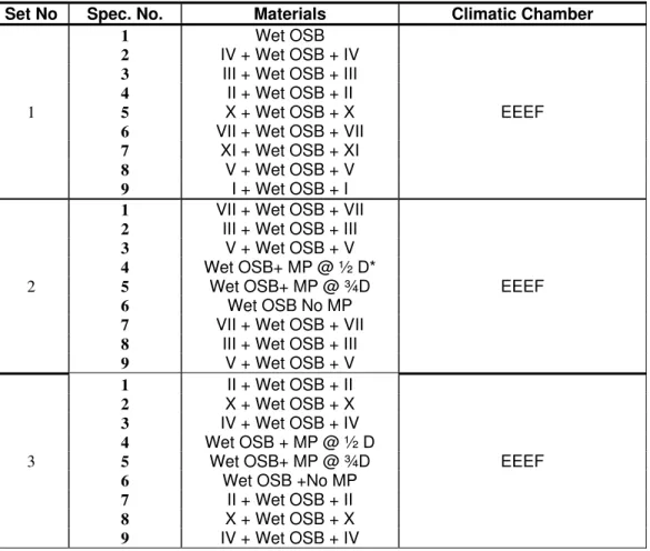
Mid-scale experiments were conducted on various types of wood-frame wall assembly components but essentially, in this series of experimental sets, the results were used to assess the drying rates of saturated OSB sheathing in contact with, or in proximity to, other OSB sheathing, and in contact with various water resistive barriers when subjected to controlled environmental conditions. The different proposed combinations are provided in Table 2, together with the nominal environmental conditions to which they were subjected. For example, the material "II + Wet OSB + II" means that, one sheathing board of saturated OSB is wrapped with sheathing membrane of type II on both sides and is subjected to controlled environmental conditions in the EEEF.
Table 2 –Mid-scale experimental sets and related component combinations and test conditions
Set No Spec. No. Materials Climatic Chamber
1
1 Wet OSB
EEEF
2 IV + Wet OSB + IV
3 III + Wet OSB + III
4 II + Wet OSB + II
5 X + Wet OSB + X
6 VII + Wet OSB + VII
7 XI + Wet OSB + XI
8 V + Wet OSB + V
9 I + Wet OSB + I
2
1 VII + Wet OSB + VII
EEEF
2 III + Wet OSB + III
3 V + Wet OSB + V
4 Wet OSB+ MP @ ½ D*
5 Wet OSB+ MP @ ¾D
6 Wet OSB No MP
7 VII + Wet OSB + VII
8 III + Wet OSB + III
9 V + Wet OSB + V 3 1 II + Wet OSB + II EEEF 2 X + Wet OSB + X 3 IV + Wet OSB + IV 4 Wet OSB + MP @ ½ D 5 Wet OSB+ MP @ ¾D
6 Wet OSB +No MP
7 II + Wet OSB + II
8 X + Wet OSB + X
9 IV + Wet OSB + IV *Refer to Moisture Pin (MP) installed at ½ depth of the thickness.
Full-scale Specimens
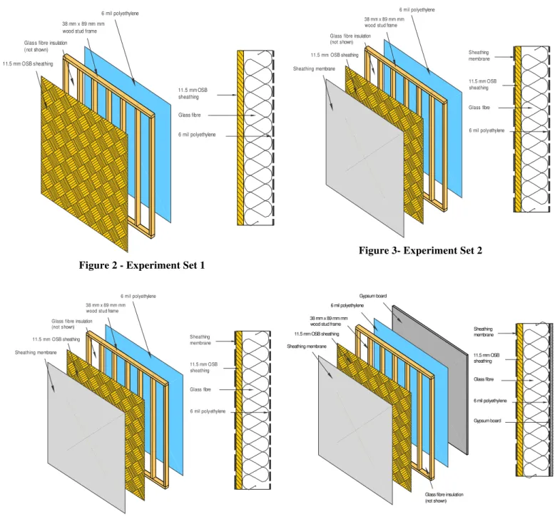
The full-scale experiments were conducted on four configurations of wood-frame wall assembly as illustrated schematically in Figure 2 to Figure 5. The results from these experiments were used to assess the drying rates of saturated OSB sheathing in contact with other building components when subjected to controlled environmental conditions in the EEEF. In the schematics provided, the various components of each of the 4 experimental sets evaluated in the full-scale tests are clearly depicted. The components used in each set are summarized in Table 3.
Table 3 – Full-scale experimental sets, related test materials combinations conditions
Set No. Materials Conditions
1 Wet OSB + Insulation + Polyethylene
EEEF 2 VII** + Wet OSB + Insulation + Polyethylene
3 IV + Wet OSB + Insulation + Polyethylene 4 IV + Wet OSB + Insulation + Polyethylene + Dry wall ** Refers to the type of water resistive barrier (WRB) – sheathing membrane
Figure 2 - Experiment Set 1
Figure 3- Experiment Set 2
Figure 4 - Experiment Set 3 Figure 5 - Experiment Set 4
6 mil polyethylene 38 mm x 89 mm mm wood stud frame
11.5 mm OSB sheathing Glass fibre insulation (not shown) 6 mil polyethylene Glass fibre 11.5 mm OSB sheathing 6 mil polyethylene 38 mm x 89 mm mm wood stud frame
11.5 mm OSB sheathing Glass fibre insulation (not shown) Sheathing membrane 6 mil polyethylene Glass fibre 11.5 mm OSB sheathing Sheathing membrane 6 mil polyethylene 38 mm x 89 mm mm wood stud frame 11.5 mm OSB sheathing
Glass fibre insulation (not shown) Sheathing membrane Gypsum board 6 mil polyethylene Glass fibre 11.5 mm OSB sheathing Sheathing membrane Gypsum board 6 mil polyethylene 38 mm x 89 mm mm wood stud frame
11.5 mm OSB sheathing Glass fibre insulation (not shown) Sheathing membrane 6 mil polyethylene Glass fibre 11.5 mm OSB sheathing Sheathing membrane
Specimen Preconditioning (Initial Conditions)
Mid-Scale Specimens
Specimens of 0.8 x 1.0-m size were immersed in a water bath (Figure 6a) for a period of 5 days to partially saturate the specimens. To ensure that water was in contact with all surfaces of the OSB specimens and to accelerate the wetting process, specimens were stacked as shown in Figure 6a which each specimen separated by aluminum angles of 1-m length. To counter the buoyancy of specimens, bricks were placed on the uppermost sample (Figure 6b). After five days, water in the bath was drained and the specimens were left in the bath for another two days to allow moisture to re-distribute evenly within the OSB. Care was taken to prevent the boards from drying out by sealing the bath lid with adhesive tape.
Figure 6a – Cross-section of immersion bath
Figure 6b – Mid-scale samples in soaking bath
Full-Scale Specimens
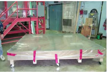
Full-scale specimens were also pre-conditioned to ensure that the OSB sheathing boards were brought to elevated moisture contents. The pre-conditioning consisted of two phases: immersion and stabilisation. The immersion phase permitted the OSB to quickly reach an elevated level of moisture content. The stabilisation phase ensured that the moisture content throughout the component reached equilibrium. The moisture content of the components was monitored on a continuous basis during the stabilization phase such that the specimen reached the desired moisture content prior to initiating the test program. The immersion phase took place in a large water tank (Figure 7) that permitted the complete immersion of the face of the specimen. The stabilization phase took place following three days of immersion. Water in the tank was drained and the specimens then remained for another two days to allow moisture to re-distribute evenly within the OSB. Care was taken to prevent the boards from drying out by sealing the tank lid with adhesive tape.
Figure 7 – Full-scale samples in soaking bath Water
Specimens Aluminum angles
Nominal Results from benchmarking exercises
Prior to providing results on the respective benchmarking exercises, information is first given on the model implementation and simulation assumptions as these offer some insights into the resulting simulations to which are compared the experimental results. Results from the mid-scale experiments are first provided followed by those obtained from tests on full-scale specimens.
Results from midscale tests
Model implementation and Simulation assumptions
The model implementation of the sheathing board, flanked on either side with a “layer’ of sheathing membrane (i.e. 3 layers: membrane, OSB, membrane), was represented using a rectangular mesh approach. This mesh was comprised of 20 nodal points along the height of the specimen (y-direction) and 16 nodal points across the depth (x-direction) for a total number of 320 nodal points for the entire representation. Membranes, installed on either side of the OSB were each comprised of 3 equidistant nodes across their depth. The OSB (thickness 11.5-mm) had 10 equidistant nodes. In the case where the response of the OSB alone was simulated, the grid representation in this instance had an expanding mesh implying that the grid density near the edges of the nodes across its depth was greater than that at the center. The surface heat transfer coefficient was 10 W/m2°C whereas the moisture transfer coefficient along the principal planar surfaces of the specimen was 4.6 x 10⁻⁷ kg/m2•s•Pa and at the top and bottom of the specimen was 7.4 x 10⁻¹⁵ kg/m2•s•Pa. Though the experimental data provided boundary conditions every 2 minutes, the time step used in the simulation was 60 minutes – this provided ample resolution in a drying process that generally took several weeks.
The assumptions under which the simulations were conducted are:
• Membranes were represented as vapour diffusion control elements.
• Contact between the membranes and the OSB sheathing was perfect (i.e. no interstitial airspace between components).
• Initial moisture content (MC) of the membrane was 0%.
Nominal results and discussion
After a number of simulations undertaken to help benchmark the model representation, it was determined that the grid size had an important effect on the drying curve derived from simulation, especially grid sizes near the “free surface” of specimens. Using a higher density grid near the “free surface” of the OSB enhances the modelling of mass transfer from the free surface to the surrounding air. The largest discrepancy between model and experiment was reduced from 22% to 12.5% by using an irregular instead of a regular mesh. This adjustment in model representation did not worsen the already good correspondence at the lower MC ranges, where the drying rate is lower.
The grid size is not the only parameter that influences the accuracy of the simulation. It must also be considered that the current simulation did not provide for an air gap to be present between the OSB sheathing. In reality, given that perfect contact between membrane and specimen does not exist, it can be assumed that an air gap does indeed exist. Consequently, it can be expected that under certain environmental conditions some condensation could occur on that side of the membrane nearest the free surface of the OSB. These conditions, and the possibility of condensation occurring, and for which an air gap is assumed, need to be further explored to determine the extent to which they are factors in providing more accurate simulation results.
A number of different scenarios were considered thus helping ensure that the hygrothermal performance of the assemblies was adequately represented. However, it must be acknowledged that in terms of the drying times, as well as the shape of the drying curve derived from these experimental sets, the overall agreement between the experimental and simulated drying curves is excellent.
Experiment Set 1
Figure 8 depicts the surrounding environmental conditions i.e. temperature (T) and relative (RH), within the EEEF.
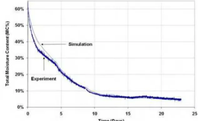
Figure 9 depicts the drying results of the OSB layer exposed to the surrounding environmental conditions within the EEEF. In this experiment, the weight of the specimens was monitored using load cells whose signals were captured through a data-logging system (the slight instability in the readings is attributed to small random errors). In this series of experiments, the initial MC of the OSB was 61%. As can be observed in Figure 9, the equilibrium MC (EMC) is achieved after 21 days (5%); the simulation is in good agreement with the experimental data. The only differences between the two drying curves manifest themselves in the first 4 days of drying, at high moisture contents; the largest difference is 5% MC, which is negligible for actual conditions.
Figure 9 – Comparison of simulated and measured drying
results of OSB layer
Figure 10– Comparison of simulated and measured drying
results of OSB layer (The OSB was wrapped on both sides with membrane III)
Figures 10 and 11 show the simulated and measured drying results for the OSB layer wrapped on both sides by membranes labeled III and II respectively. In general, the simulation curves follow the shape of the experimental data, but there are some differences in agreement. The initial MC for the OSBs (Fig. 10, membrane III; Fig. 11, membrane II) was respectively 66% and 65%. Nonetheless, the overall simulation results provided in Figures 10 and 11 show good agreement with the experimental data. The biggest difference in MC derived from these comparisons is around 6% MC. It can also be stated that, in general, all simulations provided reasonably accurate drying time for the OSB to reach their respective EMC.
Figure 11– Comparison of simulated and measured drying results of OSB layer (The OSB was wrapped on both sides with membrane II)
Figure 12– Comparison of simulated and measured drying results of OSB layer (The OSB was wrapped on both sides with membrane X) 0% 10% 20% 30% 40% 50% 60% 70% 80% 90% 100% 0 5 10 15 20 25 Time (Days) Total M o istur e content (M C%) Experiment Simulation
A comparison between simulated and experimental results for OSB wrapped with membrane X is presented in Figure 12 and that of OSB wrapped with membrane VII in Figure 13. For the OSB wrapped with membrane X, the initial MC of the OSB is 63% and the EMC (5%) is reached after 21 days. In the case of the OSB wrapped with membrane VII, a comparison of the simulation to experimental results shows that the simulation predicts the drying within an acceptable degree of error (10%). Finally, comparative results for OSB wrapped in membrane V are provided in Figure 14and show excellent agreement between the simulated drying curve and the experimental results.
Figure 13 – Comparison of simulated and measured drying results of OSB layer (The OSB was wrapped on both sides with membrane VII)
Figure14 – Comparison of simulated and measured drying results of OSB layer (The OSB was wrapped on both sides with membrane V)
Experiment Set 2
Figure 15 depicts the surrounding environmental conditions within the EEEF.
Figure 15 – Environmental Conditions of the EEEF
Nominal results for mid-scale experimental set 2 are provided in Figures 16 to 26. They include the weights of individual specimens together with resistance measurements taken across each moisture pin pair as a function of time. The moisture content (MC) was obtained using eq. 1 which was derived from the calibration curve provided in [15].
MC (%) = 100*[Log (Resistance (Ω))-9.1884] / (-14.152) (1)
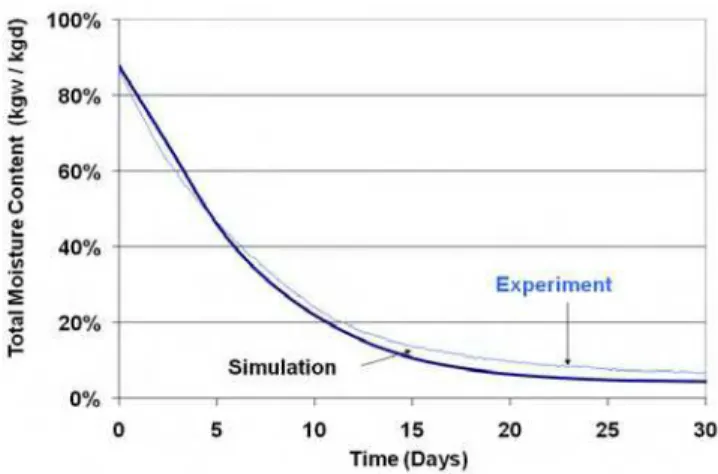
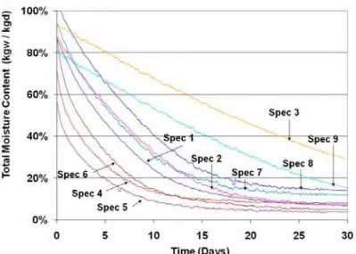
The hygrothermal simulation model hygIRC was used to estimate the drying response of nine specimens of OSB. The total moisture content as function of time of the nine (9) specimens, as determined by gravimetric analysis, is provided in Figure 16. Figure 17, shows a comparison between simulated and measured total MC of the OSB board (per 0.8 meter of specimen width) as a function of time for specimen 4. The total initial MC in the system for specimen 4 is approx. 70 % and after 30 days it drops to 7%.
Figure 16- Total moisture content as function of time of 9 test specimens determined by gravimetric analysis for Set 1
Figure17- Total moisture content as function of time of OSB layer – specimen 4 (Experiment / Simulation)
Figure 18 shows a comparison between simulated and measured total MC of the OSB board as a function of time for specimen 5. The total initial MC in the system for specimen 5 is ca. 58 % and after 30 days it drops to 5%. Figure 19 provides the simulated and experimental drying results for OSB board wrapped on both sides in membrane VII (specimen 1). The simulation curve in this figure follows the shape of the experimental data. The initial moisture content for OSB was 88%. The model predicts the same period of time to reach the equilibrium moisture content (6%). These results indicate a good agreement between results of simulation and those derived from experiment.
In general, the drying process is governed by the vapour permeability of the membrane. The higher the vapour permeability, the greater the drying rate for a given set of environmental conditions. Given that the specimens were immersed in water for 5 days and then allowed to stabilize in an enclosed environment (sealed tank), it was assumed that this period of stabilization would help assure that the initial moisture content at the start of the experiment was uniform through the thickness of the material; this was not the case in every instance. This was detected from data extracted from moisture pins installed in specimens 4, 5, 7, 8 and 9 (see Table 2). Indeed, it was observed after the period of stabilization that certain OSB specimens were, at times, wetter in certain parts of the board than in others, suggesting a non-homogeneous wetting pattern.
Figure 18- Total moisture content as function of time of OSB layer – mid-scale specimen 5 (Experiment / Simulation)
Figure 19 - Total moisture content as function of time of OSB layer wrapped on both sides with membrane VII – mid-scale specimen 1 (Experiment / Simulation)
Figure 20 shows the change in moisture content in relation to time (days) in OSB specimen 5 for each of the 6 moisture pin pairs installed at ¾ the specimen depth. As is shown in this Figure, the bottom part of the specimen dries faster than the top. This was due to the air movement in the climatic chamber that is estimated to be 1 m/s. The OSB starts drying at a significant rate (change from 27% to 10% Moisture Content) after the second day of the experiment in location 14 whereas in location 10, a similar rapid drying rate only occurs after 7 days. After the 12 days, asymptotic values of moisture content are observed at all moisture pin locations.
Based on these data it can be stated that, in general, the rapid drying rate observed was adequately described by the response obtained from the moisture pins and the drying process can thus be reasonably well ascertained based on these types of measurements.
Figure 20– Local moisture content of mid-scale specimen 5 (OSB only)
Figure 21- Local moisture content of mid-scale specimen 4 (OSB only)
The change in moisture content in relation to time of moisture pins placed at one-half the specimen depth in OSB specimen 4 is presented in Figure 21. Moisture contents at a given pin-pair location were determined by associating the resistance to a specific moisture content based on the resistance-MC calibration curve obtained from previous experiments [15].
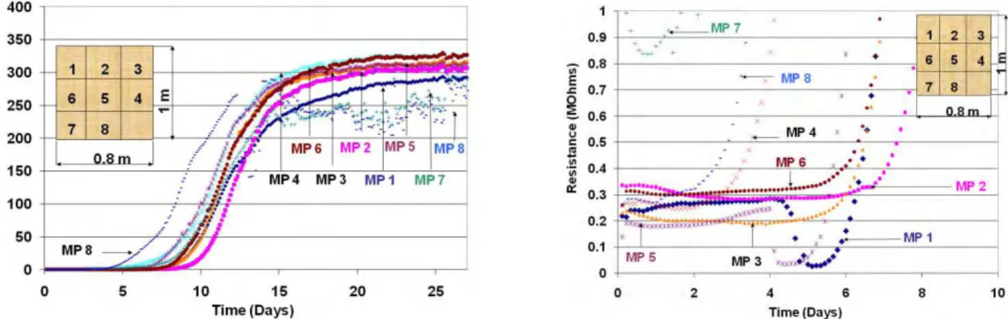
Figure 22 - Resistance Vs Time for mid-scale specimen 4, from 0-27 days
Figure 23- Resistance Vs Time for mid-scale specimen 4, from 0-10 days
Figure 22 shows the change in resistance (MΏ) in relation to time (days) in OSB specimen 4 for each of 8 moisture pin pairs installed at one-half the specimen depth. Three phases in the drying response of the specimen can be observed in this figure:
• The first phase occurs between 0 and 5 days; • The second between 5 and 15 days; and • The third between 15 and 27 days.
Figure 23 shows the first stage of drying of specimen 4, occurring in the first 5 days. After 5 days of drying all moisture pins returned to a high value of resistance indicating lower moisture content. In phase 2 of the drying process (5 to 15 days), the resistance changed rapidly from 360 kΏ to almost 5 MΏ (i.e. equivalent to 25.8 % to 15.2 % MC). After 10 days the curve continues slightly and a value of 280 MΏ (11.0 % MC) is obtained. After the 15th day, asymptotic values of resistance are observed; all the values lie between 280 MΏ and 320 MΏ (i.e. between 11.0 % and 10.6 % MC). Based on these data it can be stated that, in general, the rapid drying rate observed was adequately described by the response obtained from the moisture pins and the drying process can thus be reasonably well ascertained based on these types of measurements.
The lowest MC, i.e. the maximum resistance, is reached after 15 days of drying. These results further indicate that the process of symmetrical drying of wetted OSB proceeds very rapidly in the initial stages (i.e. first 5 days of drying) and thereafter, the rate of drying diminishes significantly. Results obtained for drying of wetted OSB wrapped with membranes VII, III, and V are presented in Figures 24, 25 and 26 respectively.
Figure 24 - Local moisture content of specimen 7 (OSB wrapped with membrane VII)
Figure 25 - Local moisture content of specimen 8 (OSB wrapped with membrane III)
Figure 24 provides the change in moisture content in relation to time, as measured across the moisture pins when installed at 1/2 the depth of specimen No. 7. In comparison to the previous results obtained for OSB not wrapped with membrane, the rate of drying is evidently lower. For specimen 7, the surface of OSB is not in direct contact with air; hence water vapour must diffuse through the membrane, which necessarily reduces the drying rate. Membrane VII has lower vapour permeability than the OSB and is also the least permeable. Similar remarks can be offered regarding the results presented in Figure 25, which represents the moisture content in relation to time of 6 moisture pins installed at one-half the OSB thickness of specimen 8 wrapped in membrane III. The drying rate is slower than the previous specimen and the reason for this is straightforward: the vapour permeability of membrane III is the lowest among the membranes tested and so is the least permeable amongst them. Hence the drying of OSB wrapped with this membrane evidently would take more time to reach the EMC than OSB wrapped with membrane VII.
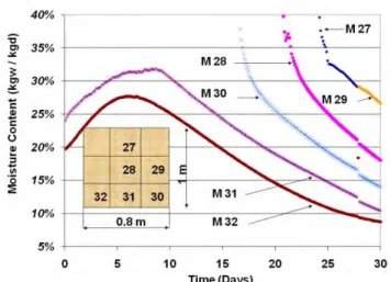
Figure 26 - Local moisture content of specimen 9 (OSB wrapped with membrane V)
Figure 26 represents the moisture content in relation to time of the 6 moisture pins installed at one-half the OSB thickness in specimen 9 wrapped in membrane V. The OSB sheathing did not dry completely after 30 days of experiment since it can be observed that the top portion (moisture pins M27, M28, M29) is still wet. Because of the low vapour permeability of membrane V, the drying rate is slower than the previous specimens. Hence the drying of OSB wrapped with this membrane evidently would take more time to reach the EMC than OSB wrapped with either membrane III or VII.
Experiment Set 3
The total moisture content as function of time of the nine (9) specimens of experimental set 3, as determined by gravimetric analysis, is provided in Figure 27. The drying process in set 3 is similar to the previous set. The higher the vapor permeability, the greater the drying rate for the given environmental conditions.
Figure 27 - Total moisture content as function of time of 9 test specimens as determined by gravimetric analysis for Set 3
RESULTS FROM FULLSCALE TESTS
Model implementation and Simulation assumptions
Four layers represented the wall assembly, specifically, layers of: sheathing membrane, sheathing board, insulation and vapor barrier (polyethylene sheet). The wall was represented in the model using a rectangular mesh comprised of 40 nodal points along the height of the specimen (y-direction) and 26 nodal points across the depth (x-direction), totaling 1040 nodal points for the entire representation. Membranes, installed on the exterior side of the OSB were each comprised of 3 equidistant nodes across their depth. The OSB (thickness 11.5-mm) had 10 equidistant nodes; the insulation, 10 equidistant nodes; the polyethylene sheet acting as an air and vapour barrier 3 equidistant nodes. In the case where the response of the OSB alone was simulated, the grid representation in this instance had an expanding mesh implying that grid density near the edges of the nodes across its depth was greater than that at the center.
The surface heat transfer coefficient was 10 W/m2°C on the single sheet of polyethylene and 12 W/m2 °C on the sheathing membrane. The moisture transfer coefficient along the principal planar surfaces of the specimen was 4.6 x 10⁻⁷ kg/m•s•Pa on the exterior, 5.5 x 10⁻⁷ kg/m•s•Pa on the interior and at the top and bottom of the specimen was 7.4 x 10⁻¹⁵ kg/m•s•Pa. Experimental data was extracted every 2 minutes whereas the time step used in the simulation, was 60 minutes, the same as was used for the mid-scale simulations and thus, as before, providing sufficient information to adequately simulate the drying process that, in this instance, also took several weeks.
The simulations were conducted under the same assumptions as those for the simulations undertaken on the mid-scale specimens; specifically:
o The membranes were represented as vapour diffusion control elements.
o The contact between the membranes and OSB sheathing was assumed to be perfect (i.e. no interstitial airspace between components).
o The initial moisture content (MC) of the membrane and polyethylene was 0%.
Nominal results and discussion
Experiment Set 1
Since the specimens were immersed in water for 2 days and then allowed to stabilise in a sealed tank, it was assumed that for all specimens the initial MC at the start of the experiment was uniform through the thickness of the material. Figure 28 shows the change in MC in the OSB derived from simulations and those from experimental results of Set 1. All results are presented as the total MC distribution over a 2.44-m width of wall as a function of time. In Figure 30, the greatest difference between the results obtained from experiment and the simulation is 4% MC. It can also be observed that an Equilibrium Moisture Content (EMC) is not reached after 16 days; it is estimated that the experiment would need to proceed to at least 40 days to reach the EMC.
Figure 28 – Comparison of the simulated and measured drying results of OSB layer
Experiment Set 2
Figure 29 shows a comparison between simulated and total measured MC of OSB derived from experimental results of Set 2. The initial total MC for both boards in the assembly, as described in the previous section, is ca. 51 %. After 33 days a MC of 16% is achieved. These results indicate good agreement between the results obtained from simulation and those derived from experiment. In fact, the greatest difference between the simulated and the experimental results after 33 days is not more than 1.4 % MC.
Figure 29— Comparison of experiment and simulated drying results in terms of total MC (%) of OSB sheathing wall components
No adjustments to the model were made to minimize the differences between results from simulation and those of the experiment. However, differences between results may be due to a number of factors the most significant are thought to be related to the manner in which the simulation at the surface of the OSB sheathing was implemented in the program. Specifically, the simulation assumes that there is perfect contact between the membrane and the sheathing board. In fact, in the real system, there always exists some interstitial space between these components. The net effect of this assumption is that the drying rate of the sheathing board in the simulation is decreased and this in-turn, underestimates the loss in moisture content over time, as is shown in Figure 29.
In general, the simulations were able to adequately predict the time required for the OSB sheathing to reach equilibrium moisture content; essentially, hygIRC is clearly able to mimic the drying process in this wall assembly. In each of the experimental steps so far reported, simulation results have shown very good agreement with those derived from experiment. Indeed, the greatest difference evident when comparing the results derived from simulation and those obtained
from experiment are ca. 5%. A number of such types of experiments have been made in the stepwise approach to help validate hygIRC.
In these experiments, local moisture content was measured using electrical resistance measurements at moisture pin pairs. These were installed in the OSB at different locations and at different depths. The results obtained using moisture pin sensors permit quantifying the moisture content of the OSB at specific locations where they are applied and from which the nominal MC distribution in the OSB can then be derived. The resistance measurements were taken across each pair of moisture pins and results were captured on a data acquisition unit (DAU). Moisture contents at a given pin-pair location were determined by associating the resistance to a specific moisture content based on the resistance-MC calibration curve obtained from other experiments [15].
Figure 30 –Zones where moisture pins were installed Figure 31 - Moisture pin locations
Figure 30 shows the wall specimen and the zone of moisture pin sensor installation. The moisture pins were installed in six specific zones, as shown in Figure 31, (see also Table 4), each zone representative of the size of specimen used in the mid-scale tests (i.e. 0.8-m by1-m). The MC data retrieved from each zone provides the basic information needed to map the MC distribution over the entire wall.
Table 4 – MP locations inserted in 6 zones of the wall assembly
Zone No. Description Pin No. 1-8 Pin No. 9-16 Pin No. 17-24 Pin No. 25-32
Zone1
Bottom, left
1, 2, 3,
10, 11, 12,
16
Zone 2
Bottom, center
4, 5, 6
13, 14
17,18
Zone 3
Bottom, right
7, 8
9, 15
19, 20, 21
Zone 4
Top, left
26, 27
Zone 5
Top, centre
23, 24
27, 28, 31,
32
Zone 6
Top, right
25, 29, 30
All calibration was completed up to 120 MΩ (i.e. from saturation to 12 % MC). At this resistance level, resistance values above this limit (or MC values below 12%) are not being used in the analysis to benchmark the results derived from computer simulation. However, despite the fact that values of resistance in excess of this limit are not being relied upon for benchmarking purposes, the information is nonetheless useful to further understand the test results.
Evident on all the figures representative of full-scale results is that on day 10 of the experiments a singular peak occurred. It can be explained by either of two scenarios:
• The electrical circuit for moisture pins attained a limiting value; or a • Physical phenomenon happened at that time (e.g. more ventilation).
Figure 32- Resistance versus time of the 7 moisture pins in zone 1
Figure 33- Moisture content versus time of the 7 moisture pins in zone 1
Figure 32 shows the change in resistance (MΏ) in relation to time (days) in zone 1 of the OSB sheathing for each 7 moisture pin pairs installed at one-half the specimen depth. The drying appears to be very rapid; after 10 days the resistance values across moisture pin sensors are between 80 MΩ and 700 MΩ for all specimens. The MC in this wall zone is between 12.7 % and 10 % MC.
Figure 33 shows the drying curve for the OSB in Zone 1 of the panel in terms of change in MC over time. In Zone 1, it is apparent that the moisture pins located at the top are first to indicate drying whereas those located at the bottom follow after this process is initiated. This indicates that the bottom has a tendency to stay wet while the top dries out. Figure 32 provides a similar response to that apparent from the results given in Figure 33.
The same phenomena are evident from data taken from zone 2 as given in Figures 34 to37; Figures 34 and 35 provide information on the entire drying phase of the experiment whereas Figures 36 and 36 focus on the initial portion of the experiment and over the first 10 days of drying
Figure 34 - Resistance versus time of the 7 moisture pins in zone 2
Figure 35 - Moisture content versus time of the 7 moisture pins in zone 2
Figure 34 shows the drying curve for the OSB component in Zone 2 in terms of change in resistance (MΏ) over time; the information presented in this Figure is similar to that of Figure 32, although Figure 34 only provides the 10 first days over which the greatest rate of drying occurs. Figure 35 shows the drying curve for the OSB in Zone 2 of the panel in terms of change in MC over time.
Figure 36 - Resistance versus time of the 7 moisture pins in zone 2
Figure 37 - Moisture content versus time of the 7 moisture pins in zone 2
Figure 38 shows the drying curve of the OSB at two locations: (1) bottom location of the wall in Zone 1 (moisture pin (MP) #5), and; (2) top location of the wall in Zone 5 (MP #31). Based on this information, it is evident that the bottom of the wall is drying slower than the top even if these two locations have started at the same equilibrium moisture content (EMC) of 25% MC. The results depicted in this figure show the effect of gravity, the redistribution of moisture within the assembly, and as well, the effect of air circulation within the EEEF.
After 5 days of drying, MP #31 located at the top, indicates that the OSB at this location is dry, and whereas for MP #5 located at the bottom, shows 25% MC, indicating that this location of the OSB is still wet (over 20% of MC). After 10 days both moisture pins (MP) locations reached the EMC as is evident for the whole assembly.
Figure 39 shows a drying curve for two adjacent locations at the center of the OSB panel, specifically, MP #23 (Zone 5) and MP #18 (Zone 2). This figure shows that during the drying process part of the moisture is evaporated by vapour diffusion and another part is transported to the next node or location and thereafter, redistributed within the assembly. This is especially evident during days 5 and 8.
Figure 38 – Moisture content of two extreme moisture pin locations (Top and Bottom)
Figure 39 – Moisture content of two adjacent nodes
Experiment Set 3
Figure 40 shows results from experimental Set 3 in which a comparison is provided of the total MC of OSB as obtained from simulation results and that from the experimental work. The total MC in the system is initially approximately 70 %; after 28 days it reaches a value of 24%. The test was stopped after 4 weeks because of practical considerations. Again, these results indicate an excellent agreement between results of simulation and those derived from experiment given that the difference between results is no greater than 5 %.
Figure 40 — Comparison of experiment and simulated drying results in terms of total MC (%) of OSB sheathing wall components
Experiment Set 4
Results of Experimental Set 4, provided in Figure 41, show the total MC of the OSB obtained from simulated results as compared to those derived from experimental work. The total MC in the system is initially approximately 36 %; after 25 days it reaches a MC of 28%. Again, these results indicate an excellent agreement between results of simulation and those derived from experiment given that the difference between results is no greater than 3 %.
Figure 41 — Comparison of experiment and simulated drying results in terms of total MC (%) of OSB sheathing wall components
CONCLUDING REMARKS
The results presented in this document offer an overview of the work carried out on both mid- and full-scale drying experiments. The most apparent observation is that the moisture pins provide quantitative information on the moisture content of the OSB in each zone over the time the drying experiment is conducted. Another noteworthy observation is that in mid-scale experiments the effect of the membrane on the drying process is quite evident: OSB wrapped with membrane will necessarily dry slower than the OSB alone. Another singular item from mid-scale tests is that there are no evident gravity effects in the specimens tested, however, the effect is noticeable in results obtained on full-scale specimens (bottom is wet whereas top is dry). In general, the drying process is governed by the vapour permeability of the membrane. The higher the vapour permeability, the greater the drying rate for a given set of environmental conditions. The rate of faster drying is shown since the first day of the experiment such as shown in Figure 27.
The hygrothermal simulation model hygIRC has been used in various other studies as the primarily analytical tool to conduct a parametric study to assess the hygrothermal performance of various wall assembly types subjected to different North American climatic conditions [16]. It has been demonstrated that the overall agreement between the experimental and simulated drying curves is good in terms of the time to reach equilibrium moisture content, as well as the shape of the drying curve derived from these experimental sets. As has been demonstrated from comparison of results obtained from simulation to that of controlled laboratory experiments, hygIRC can adequately duplicate the response of the modeled assemblies and thus help predict hygrothermal behaviour of wall components when subjecting the components to simulated climatic conditions.
REFERENCES
[1] Maref, W.; Kumaran, M.K.; Lacasse, M.A.; Swinton, M.C.; van Reenen, D., "Laboratory measurements and benchmarking of an advanced hygrothermal model," Proceedings of the Twelfth International Heat Transfer Conference
(IHTC12), Assembly for International Heat Transfer Conferences (AIHTC), August 18, 2002, Grenoble, France, pp.
117-122
[2] Maref, W. Lacasse, M.A. and Booth, D.G., “Benchmarking of IRC's Advanced Hygrothermal Model - hygIRC Using Mid- and Large-Scale Experiments”, Research Report No. RR-126, Institute for Research in Construction, National Research Council Canada, Ottawa, December, 2002, p. 38.
[
3
] Maref, W., Lacasse, M.A. and Booth, D.G., “Executive Summary of Research Contributions Related to Moisture Management of Exterior Wall Systems (MEWS) - Modeling, Experiments, and Benchmarking”, Research Report No. RR-127, Institute for Research in Construction, National Research Council Canada, Ottawa, December, 2002, p. 15, [4] Maref Maref, W.; Lacasse, M.A.; Kumaran, M.K.; Swinton, M.C., "Benchmarking of the advanced hygrothermalmodel-hygIRC with mid-scale experiments," Proceedings of the Canadian Conference on Building Energy Simulation (eSim 2002), International Building Performance Simulation Association(IBPSA), September 11-13, 2002, Montreal, Canada, pp. 171-176
[5] ] Salonvaara, M. and A.N. Karagiozis, “Moisture Transport in Building Envelopes using an Approximate Factorization Solution Method”, Second Annual Conference of the CFD Society of Canada, Toronto, June 1-3, 1994, pp. 317- 326. [6] Karagiozis, A.N., M.H. Salonvaara and M.K. Kumaran, “The Effect of Waterproof Coating on Hygrothermal
Performance of high-rise Wall Structure,” Proceedings of the International Conference on the Thermal Performance of the Exterior Envelopes of Buildings VI, ASHRAE/DOE/BTECC Conference, Clearwater, FL, USA, December 4-8, 1995, pp. 391-398.
[7] Karagiozis, A. N. and M.K. Kumaran, “Applications of Hygrothermal Models to Building Envelope Design Guidelines”, Fourth Canada/Japan Housing R&D Workshop, Sapporo, Japan, November 16-21, 1997, pp. III-25 to III-36.
[8] Heinz R. Trechsel (Ed.), Moisture Control in Buildings, ASTM Manual Series MNL18, American Society for Testing and Materials, West Conshohocken, PA, 1994, 484 p.
[9] Tariku, F.; Cornick, S.; Lacasse, M., “Simulation of Wind-Driven Rain Effects on the Performance of a Stucco-Clad Wall”, Proceedings of the International Conference on the Thermal Performance of the Exterior Envelopes of Whole Buildings X, ASHRAE/DOE/BTECC Conference, Clearwater, FL, USA, December 2-7, 2007, pp. 1-15.
[10] Maref, W., Lacasse, M., Booth, D., Nicholls, M. and O'Connor, T., “Automated weighing and moisture sensor system to assess the hygrothermal response of wood-sheathing and combined membrane sheathing wall components”, Proceedings of the 11th Symposium for Building Physics, Dresden, Germany, Technical University Dresden, September 26-27, 2002, pp. 595-604.
[11] Hagentoft, C-E.; Adan, O.; Adl-Zarrabi, B.; Becker, R.; Brocken, H.; Carmeliet, J.; Djebbar, R.; Funk, M.; Grunewald, J.; Hens, H.; Kumaran, M.K.; Roels, S.; Kalagasidis, A.S.; Shamir, D., “Assessment Method of Numerical Prediction Models for Combined Heat, Air and Moisture Transfer in Building Components: Benchmarks for One-Dimensional Cases”, European Community Project HAMSTAD Technology Implementation Plan, Journal of Thermal Envelope and Building Science, v. 27, no. 4, April 2004, pp. 327-335.
[12] Tariku, F.; Kumaran, M. K. (2006), “Hygrothermal Modeling of Aerated Concrete Wall and Comparison With Field Experiment”, Proceedings of the Third International Building Physics Conference - Research in Building Physics and Building Engineering, International Association of Building Physics (IABP), August 27-31, Montreal, Canada, pp. 321-328..
[13] Maref, W., Lacasse, M.A. and Krouglicof, N., "A Precision weighing system for helping assess the hygrothermal response of full-scale wall assemblies," Proceedings of the International Conference on Performance of Exterior Envelopes of Whole Building VIII: Integration of Building Envelopes, ASHRAE/DOE/BTECC Conference, Clearwater Beach, FL, USA, December 12, 2001, pp. 1-7.
[14] Kumaran, M.K., Lackey, J., Normandin, N., van Reenen, D., Tariku, F. (2002), "Summary Report from Task 3 of MEWS Project At the Institute for Research in Construction - Hygrothermal Properties of Several Building Materials", Research
Report No. 110, Institute for Research in Construction, National Research Council, Ottawa, Canada, pp. 1-73.
[15] Maref, W. and Lacasse, M.A., “Experimental Assessment of Hygrothermal Properties of Wood-Frame Wall Assemblies / Moisture Content Calibration Curve of OSB Using Moisture Pins”, Submitted to the Second Symposium on
Heat-Air-Moisture Transport: Measurement and Implication in Buildings, ASTM Committee C16 on Thermal Insulation,
[16] Beaulieu, P.; Bomberg, M.T.; Cornick, S.M.; Dalgliesh, W.A.; Desmarais, G.; Djebbar, R.; Kumaran, M.K.; Lacasse, M.A.; Lackey, J.C.; Maref, W.; Mukhopadhyaya, P.; Nofal, M.; Normandin, N.; Nicholls, M.; O'Connor, T.; Quirt, J.D.; Rousseau, M.Z.; Said, M.N.; Swinton, M.C.; Tariku, F.; van Reenen, D., “Final Report from Task 8 of MEWS Project (T8-03) - Hygrothermal Response of Exterior Wall Systems to Climate Loading: Methodology and Interpretation of Results for Stucco, EIFS, Masonry and Siding-Clad Wood-Frame Walls”, Research Report No. RR-118, Institute for Research in Construction, National Research Council Canada, Ottawa, Canada, November 01, 2002, 183 p.
APPENDIX A
Figure A1
-
Sorption curve for oriented-strand-board (OSB) – MC as a function of % RHFigure A2
- S
orption curve for sheathing membranes II, III and V– MC as a function of % RH.Figure A3
-
Sorption curves for sheathing membranes VII and X– MC as a function of % RHFigure A4