Peter J. nolan
state university of new york - Farmingdale
Copyright © 2014 by Physics Curriculum & Instruction, Inc. www.PhysicsCurriculum.com
Produced in the United States of America
All Rights Reserved. This electronic textbook is protected by United States and Inter-national Copyright Law and may only be used in strict accordance with the accompa-nying license agreement. Unauthorized duplication and/or distribution of this electronic textbook is a violation of copyright law and subject to severe criminal penalties.
FUNDAMENTALS OFMODERNPHYSICS First Edition
BYPETERJ. NOLAN
Single-Copy License
Physics Curriculum & Instruction hereby grants you a perpetual license, free of charge, to use Fundamentals of Modern Physics by Peter J. Nolan textbook(hereafter referred to as “the book”). The terms of this agree-ment are as follows:
I. Physics Curriculum & Instruction retains full copyright and all rights to the book. No rights to the book are granted to any other entity under this agreement.
II. The user may download the book for his or her own personal use only, and may print a single copy for per-sonal use only. A single copy of the book may be stored on the user’s computer or other electronic device. III. The book may not be distributed or resold in any manner. Physics Curriculum & Instruction is the only en-tity permitted to distribute the book. All access to the book must take place through the Physics Curriculum & Instruction website.
IV. No portion of the book may be copied or extracted, including: text, equations, illustrations, graphics, and photographs. The book may only be used in its entirety.
V. If the book is to be utilized by an institution for a student course, it may not be distributed to students through a download site operated by the institution or any other means. Student access to the book may only take place through the Physics Curriculum & Instruction website.
Fundamentals of Modern Physics by Peter J. Nolan is published and copyrighted by Physics Curriculum & In-struction and is protected by United States and International Copyright Law. Unauthorized duplication and/or distribution of copies of this electronic textbook is a violation of copyright law and subject to severe criminal penalties.
For further information or questions concerning this agreement, contact: Physics Curriculum & Instruction
www.PhysicsCurriculum.com email: info@physicscurriculum.com tel: 952-461-3470
Cover
License Agreement Preface
A Special Note to the Student Interactive Examples with Excel
1
special Relativity1.1 Introduction to Relative Motion 1.2 The Galilean Transformations of
Classical Physics
1.3 The Invariance of the Mechanical Laws of Physics under a Galilean Transformation 1.4 Electromagnetism and the Ether
1.5 The Michelson-Morley Experiment 1.6 The Postulates of the Special Theory
of Relativity
1.7 The Lorentz Transformation 1.8 The Lorentz-Fitzgerald Contraction 1.9 Time Dilation
1.10 Transformation of Velocities
1.11 The Law of Conservation of Momentum and Relativistic Mass
1.12 The Law of Conservation of Mass-Energy The Language of Physics
Summary of Important Equations Questions and Problems for Chapter 1 Interactive Tutorials
2
spacetime and General Relativity2.1 Spacetime Diagrams 2.2 The Invariant Interval
2.3 The General Theory of Relativity
2.4 The Bending of Light in a Gravitational Field 2.5 The Advance of the Perihelion of
the Planet Mercury 2.6 The Gravitational Red Shift 2.7 The Shapiro Experiment Essay: The Black Hole
The Language of Physics
Summary of Important Equations Questions and Problems for Chapter 2 Interactive Tutorials
3
Quantum Physics3.1 The Particle Nature of Waves 3.2 Blackbody Radiation
3.3 The Photoelectric Effect 3.4 The Properties of the Photon 3.5 The Compton Effect
3.6 The Wave Nature of Particles
3.7 The Wave Representation of a Particle 3.8 The Heisenberg Uncertainty Principle 3.9 Different Forms of the Uncertainty Principle 3.10 The Heisenberg Uncertainty Principle
and Virtual Particles
3.11 The Gravitational Red Shift by the Theory of Quanta 3.12 An Accelerated Clock The Language of Physics
Summary of Important Equations Questions and Problems for Chapter 3 Interactive Tutorials
4
Atomic Physics4.1 The History of the Atom 4.2 The Bohr Theory of the Atom
4.3 The Bohr Theory and Atomic Spectra 4.4 The Quantum Mechanical Model of
the Hydrogen Atom
4.5 The Magnetic Moment of the Hydrogen Atom 4.6 The Zeeman Effect
4.7 Electron Spin
4.8 The Pauli Exclusion Principle and the Periodic Table of the Elements Essay: Is This World Real or Just an Illusion? The Language of Physics
Summary of Important Equations Questions and Problems for Chapter 4 Interactive Tutorials
C
Click on any topic below to be brought to that page. To return to this page, type “i” into the page number field.
5
nuclear Physics5.1 Introduction 5.2 Nuclear Structure 5.3 Radioactive Decay Law 5.4 Forms of Radioactivity 5.5 Radioactive Series
5.6 Energy in Nuclear Reactions 5.7 Nuclear Fission
5.8 Nuclear Fusion 5.9 Nucleosynthesis Essay: Radioactive Dating The Language of Physics
Summary of Important Equations Questions and Problems for Chapter 5 Interactive Tutorials
6
elementary Particle Physics and the Unification of the Forces6.1 Introduction
6.2 Particles and Antiparticles 6.3 The Four Forces of Nature 6.4 Quarks
6.5 The Electromagnetic Force 6.6 The Weak Nuclear Force 6.7 The Electroweak Force 6.8 The Strong Nuclear Force 6.9 Grand Unified Theories (GUT)
6.10 The Gravitational Force and Quantum Gravity 6.11 The Superforce—Unification of All the Forces Essay: The Big Bang Theory
The Language of Physics
Questions and Problems for Chapter 6 Bibliography
This book is dedicated to my family— my wife Barbara,
my sons,
Thomas, James, John and Kevin, my daughters’ in-law,
Joanne and Nancy, my grandchildren,
Preface
This text gives a good, traditional coverage for students of Modern Physics. The organization of the text follows the traditional sequence of Special Relativity, General Relativity, Quantum Physics, Atomic Physics, Nuclear Physics, and Elementary Particle Physics and the Unification of the Forces. The emphasis throughout the book is on simplicity and clarity.
There are a large number of diagrams and illustrative problems in the text to help students visualize physical ideas. Important equations are highlighted to help students find and recognize them. A summary of these important equations is given at the end of each chapter.
To simplify the learning process, every illustrative example in the textbook is linked to an Excel spreadsheet (Microsoft Excel must be installed on the computer). These Interactive Examples will allow the student to solve the example problem in the textbook, with all the in-between steps, many times over but with different numbers placed in the problem. More details on these Interactive Examples can be found in the section “Interactive Examples with Excel" at the end of the Preface.
Students sometimes have difficulty remembering the meanings of all the vocabulary associated with new physical ideas. Therefore, a section called The Language of Physics, found at the end of each chapter, contains the most important ideas and definitions discussed in that chapter.
To comprehend the physical ideas expressed in the theory class, students need to be able to solve problems for themselves. Problem sets at the end of each chapter are grouped according to the section where the topic is covered. Problems that are a mix of different sections are found in the Additional Problems section. If you have difficulty with a problem, refer to that section of the chapter for help. The problems begin with simple, plug-in problems to develop students’ confidence and to give them a feel for the numerical magnitudes of some physical quantities. The problems then become progressively more difficult and end with some that are very challenging. The more difficult problems are indicated by a star (*). The starred problems are either conceptually more difficult or very long. Many problems at the end of the chapter are very similar to the illustrative problems worked out in the text. When solving these problems, students can use the illustrative problems as a guide, and use the Interactive Examples as a check on their work.
A section called Interactive Tutorials, which also uses Excel spreadsheets to solve physics problems, can be found at the end of the problems section in each chapter. These Interactive Tutorials are a series of problems, very much like the Interactive Examples, but are more detailed and more general. More details on these Interactive Tutorials can be found in the section “Interactive Tutorials with Excel” at the end of the Preface.
A series of questions relating to the topics discussed in the chapter is also included at the end of each chapter. Students should try to answer these questions to see if they fully understand the ramifications of the theory discussed in the
conceptually more difficult or will entail some outside reading. These more difficult questions are also indicated by a star (*).
In this book only SI units will be used in the description of physics. Occasionally, a few problems throughout the book will still have some numbers in the British Engineering System of Units. When this occurs the student should convert these numbers into SI units, and proceed in solving the problem in the International System of Units.
A Bibliography, given at the end of the book, lists some of the large number of books that are accessible to students taking modern physics. These books cover such topics in modern physics as relativity, quantum mechanics, and elementary particles. Although many of these books are of a popular nature, they do require some physics background. After finishing this book, students should be able to read any of them for pleasure without difficulty.
A Special Note to the Student
“One thing I have learned in a long life: that all our science measured against reality, is primitive and childlike--and yet it is the most precious thing we have.”
Albert Einstein
as quoted by Banesh Hoffmann in Albert Einstein, Creator and Rebel
The language of physics is mathematics, so it is necessary to use mathematics in our study of nature. However, just as sometimes “you cannot see the forest for the trees,” you must be careful or “you will not see the physics for the mathematics.” Remember, mathematics is only a tool used to help describe the physical world. You must be careful to avoid getting lost in the mathematics and thereby losing sight of the physics. When solving problems, a sketch or diagram that represents the physics of the problem should be drawn first, then the mathematics should be added.
Physics is such a logical subject that when a student sees an illustrative problem worked out, either in the textbook or on the blackboard, it usually seems very simple. Unfortunately, for most students, it is simple only until they sit down and try to do a problem on their own. Then they often find themselves confused and frustrated because they do not know how to get started.
If this happens to you, do not feel discouraged. It is a normal phenomenon that happens to many students. The usual approach to overcoming this difficulty is going back to the illustrative problem in the text. When you do so, however, do not look at the solution of the problem first. Read the problem carefully, and then try to solve the problem on your own. At any point in the solution, when you cannot proceed to the next step on your own, peek at that step and only that step in the
illustrative problem. The illustrative problem shows you what to do at that step. Then continue to solve the problem on your own. Every time you get stuck, look again at the appropriate solution step in the illustrative problem until you can finish the entire problem. The reason you had difficulty at a particular place in the problem is usually that you did not understand the physics at that point as well as you thought you did. It will help to reread the appropriate theory section. Getting stuck on a problem is not a bad thing, because each time you do, you have the opportunity to learn something. Getting stuck is the first step on the road to knowledge. I hope you will feel comforted to know that most of the students who have gone before you also had these difficulties. You are not alone. Just keep trying. Eventually, you will find that solving physics problems is not as difficult as you first thought; in fact, with time, you will find that they can even be fun to solve. The more problems that you solve, the easier they become, and the greater will be your enjoyment of the course.
Interactive Examples with Excel
The Interactive Examples in the book will allow the student to solve the example problem in the textbook, with all the in-between steps, many times over but with different numbers placed in the problem (Microsoft Excel must be installed on the computer). Figure 1 shows an example from Chapter 1 of the textbook for solving a problem dealing with the Lorentz contraction. It is a problem in special relativity in which a man on the earth measures an event at a particular point from him at a particular time. If a rocket ship flies over the man at a particular speed, what coordinates does the astronaut in the rocket ship attribute to this event?
The example in the textbook shows all the steps and reasoning done in the solution of the problem.
Example 1.5
Lorentz transformation of coordinates. A man on the earth measures an event at a point 5.00 m from him at a time of 3.00 s. If a rocket ship flies over the man at a speed of 0.800c, what coordinates does the astronaut in the rocket ship attribute to this event?
The location of the event, as observed in the moving rocket ship, found from equation 1.49, is 2 2 ' 1 / x vt x v c − = −
Solution
8 2 2 5.00 m (0.800)(3.00 10 m/s)(3.00 s) ' 1 (0.800 ) / x c c − × = − = −1.20 × 10⁹ m
This distance is quite large because the astronaut is moving at such high speed. The event occurs on the astronaut’s clock at a time
2 2 2 / ' 1 / t vx c t v c − = − 8 8 2 2 2 3.00 s (0.800)(3.00 10 m/s)(5.00 m)/(3.00 10 m/s) 1 (0.800 ) /c c − × × = − = 5.00 s Go to Interactive Example
Figure 1 Example 1.5 in the textbook.
The last sentence in blue type in the example allows the student to access the interactive example for this same problem. Clicking on the blue sentence opens the spreadsheet shown in figure 2. Notice that the problem is stated in the identical manner as in the textbook. Directly below the stated problem is a group of yellow-colored cells labeled Initial Conditions. Into these yellow cells are placed the numerical values associated with the particular problem. The problem is now solved in the identical way it is solved in the textbook. Words are used to describe the physical principles and then the equations are written down. Then the in-between steps of the calculation are shown in light green-colored cells, and the final result of the calculation is shown in a light blue-colored cell. The entire problem is solved in this manner, as shown in figure 2. If the student wishes to change the problem by using a different initial condition, he or she then changes these values in the yellow-colored cells of the initial conditions. When the initial conditions are changed the spreadsheet recalculates all the new in-between steps in the problem and all the new final answers to the problem. In this way the problem is completely interactive. It changes for every new set of initial conditions. The Interactive Examples make the book a living book. The examples can be changed many times over to solve for all kinds of special cases.
"The Fundamentals of the Theory of
Modern Physics"
Dr. Peter J. Nolan, Prof. Physics
Farmingdale State College, SUNY
Chapter 1 Special Relativity
Computer Assisted Instruction
Interactive Examples
Example 1.5
Lorentz transformation of coordinates. A man on the earth measures an event at a
point 5.00 m from him at a time of 3.00 s. If a rocket ship flies over the man at a speed of 0.800c, what coordinates does the astronaut in the rocket ship attribute to this event?
Initial Conditions
x = 5 m t = 3 s
v = 0.8 c = 2.4E+08 m/s c = 3.00E+08 m/s
Solution.
The location of the event, as observed in the moving rocket ship, found from equation 1.49, is
x' = (x - v t) /sqrt[1 - v2 / c2]
x' = [( 5 m) - ( 2.4E+08 m/s) x ( 3 s) ] / sqrt[1 - ( 0.8 c)2 / ( 1 c)2} ]
x' = -1.20E+09 m
This distance is quite large because the astronaut is moving at such high speed. The event occurs on the astronaut's clock at a time
t' = ( t - v x /c2) / sqrt[1 - v2 / c2]
t' = [( 3 s) - ( 2.4E+08 m/s) x ( 5 m) / ( 3.00E+08 m/s)2] / sqrt[1 - ( 2.40E+08 m/s)2 / ( 3.00E+08 c)2} ]
t' = 5 s
These Interactive Examples are a very helpful tool to aid in the learning of modern physics if they are used properly. The student should try to solve the particular problem in the traditional way using paper and a calculator. Then the student should open the spreadsheet, insert the appropriate data into the Initial Conditions cells and see how the computer solves the problem. Go through each step on the computer and compare it to the steps you made on paper. Does your answer agree? If not, check through all the in-between steps on the spreadsheet and your paper and find where your made a mistake. Do not feel bad if you make a mistake. There is nothing wrong in making a mistake, what is wrong is not learning from your mistake. Now that you understand your mistake, repeat the problem using different Initial Conditions on the spreadsheet and your paper. Again check your answers and all the in-between steps. Once you are sure that you know how to solve the problem, try some special cases. What would happen if you changed an angle, a weight, a force? In this way you can get a great deal of insight into the physics of the problem and also learn a great deal of modern physics in the process.
You must be very careful not to just plug numbers into the Initial Conditions and look at the answers without understanding the in-between steps and the actual physics of the problem. You will only be deceiving yourself. Be careful, these spreadsheets can be extremely helpful if they are used properly.
We should point out two differences in a text example and in a spreadsheet example. Powers of ten that are used in scientific notation in the text are written with the capital letter E in the spreadsheet. Hence, the number 5280, written in scientific notation as 5.280 × 10³, will be written on the spreadsheet as 5.280E+3. Also, the square root symbol, , in the textbook is written as sqrt[ ] in a spreadsheet. Finally, we should note that the spreadsheets are “protected” by allowing you to enter data only in the designated light yellow-colored cells of the Initial Conditions area. Therefore, the student cannot damage the spreadsheets in any way, and they can be used over and over again.
Interactive Tutorials with Excel
Besides the Interactive Examples in this text, I have also introduced a section called Interactive Tutorials at the end of the problem section in each chapter. These Interactive Tutorials are a series of problems, very much like the Interactive Examples, but are more detailed and more general.
To access the Interactive Tutorial, the student will click on the sentence in blue type at the end of the Interactive Tutorials section. Clicking on the blue sentence opens the appropriate spreadsheet.
Figure 3 show a typical Interactive Tutorial for problem 46 in chapter 1. It shows the change in mass of an object when it's in motion. When the student opens this particular spreadsheet, he or she sees the problem stated in the usual manner.
"The Fundamentals of the Theory of
Modern Physics"
Dr. Peter J. Nolan, Prof. Physics
Farmingdale State College, SUNY
Chapter 1 Special Relativity
Computer Assisted Instruction
Interactive Tutorial
46. Relativistic mass. A mass at rest has a value mo = 2.55 kg. Find the relativistic
mass m when the object is moving at a speed v = 0.355 c.
Initial Conditions
mo = 2.55 kg c = 3.00E+08 m/s
v = 3.55E-01 c = 1.07E+08 m/s
For speeds that are not given in terms of the speed of light c use the following converter to find the equivalent speed in terms of the speed of light c. Then place the equivalent speed into the yellow cell for v above.
v = 1610 km/hr = 447.58 m/s = 1.49E-06 c
v = 1.61E+06 m/s = 5.37E-03 c The relativistic mass is given by equation 1.86 as
m = mo / sqrt[1 - (v2)/(c2)]
m = ( 2.55 kg)/sqrt[1 - ( 1.07E+08 m/s)2 / ( 3.00E+08 m/s)2] m = 2.7276628 kg
Figure 3 A typical Interactive Tutorial.
Directly below the stated problem is a group of yellow-colored cells labeled Initial Conditions.
Into these yellow cells are placed the numerical values associated with the particular problem. For this problem the initial conditions consist of the rest mass of the object, it speed, and the speed of light as shown in figure 3. The problem is now solved in the traditional way of a worked out example in the book. Words are used to describe the physical principles and then the equations are written down. Then the in-between steps of the calculation are shown in light green-colored cells, and the final result of the calculation is shown in a light blue-green-colored cell. The entire problem is solved in this manner as shown in figure 3. If the student wishes
to change the problem by using a different initial mass or speed, he or she then changes these values in the yellowed-colored cells of the initial conditions. When the initial conditions are changed the spreadsheet recalculates all the new in-between steps in the problem and all the new final answers to the problem. In this way the problem is completely interactive. It changes for every new set of initial conditions. The tutorials can be changed many times over to solve for all kinds of special cases.
And now in our time, there has been unloosed a cataclysm which has swept away space, time, and matter hitherto regarded as the firmest pillars of natural science, but only to make place for a view of things of wider scope, and entailing a deeper vision. This revolution was promoted essentially by the thought of one man, Albert Einstein.
Hermann Weyl - Space-Time-Matter
1.1 Introduction to Relative Motion
Relativity has as its basis the observation of the motion of a body by two different observers in relative motion to each other. This observation, apparently innocuous when dealing with motions at low speeds has a revolutionary effect when the objects are moving at speeds near the velocity of light. At these high speeds, it becomes clear that the simple concepts of space and time studied in Newtonian physics no longer apply. Instead, there becomes a fusion of space and time into one physical entity called spacetime. All physical events occur in the arena of spacetime. As we shall see, the normal Euclidean geometry, studied in high school, that applies to everyday objects in space does not apply to spacetime. That is, spacetime is non-Euclidean. The apparently strange effects of relativity, such as length contraction and time dilation, come as a result of this non-Euclidean geometry of spacetime.
The earliest description of relative motion started with Aristotle who said that the earth was at absolute rest in the center of the universe and everything else moved relative to the earth. As a proof that the earth was at absolute rest, he reasoned that if you throw a rock straight upward it will fall back to the same place from which it was thrown. If the earth moved, then the rock would be displaced on landing by the amount that the earth moved. This is shown in figures 1.1(a) and 1.1(b).
Figure 1.1 Aristotle’s argument for the earth’s being at rest.
Based on the prestige of Aristotle, the belief that the earth was at absolute rest was maintained until Galileo Galilee (1564-1642) pointed out the error in Aristotle’s reasoning. Galileo suggested that if you throw a rock straight upward in
a boat that is moving at constant velocity, then, as viewed from the boat, the rock goes straight up and straight down, as shown in figure 1.2(a). If the same
Figure 1.2 Galileo’s rebuttal of Aristotle’s argument of absolute rest.
projectile motion is observed from the shore, however, the rock is seen to be displaced to the right of the vertical path. The rock comes down to the same place on the boat only because the boat is also moving toward the right. Hence, to the observer on the boat, the rock went straight up and straight down and by Aristotle’s reasoning the boat must be at rest. But as the observer on the shore will clearly state, the boat was not at rest but moving with a velocity v. Thus, Aristotle’s argument is not valid. The distinction between rest and motion at a constant velocity, is relative to the observer. The observer on the boat says the boat is at rest while the observer on the shore says the boat is in motion. We then must ask, is there any way to distinguish between a state of rest and a state of motion at constant velocity?
Let us consider Newton’s second law of motion as studied in general physics,
F = ma
If the unbalanced external force acting on the body is zero, then the acceleration is also zero. But since a = dv/dt, this implies that there is no change in velocity of the body, and the velocity is constant. We are capable of feeling forces and accelerations but we do not feel motion at constant velocity, and rest is the special case of zero constant velocity. Recall from general physics, concerning the weight of a person in an elevator, the scales read the same numerical value for the weight of the person when the elevator is either at rest or moving at a constant velocity. There is no way for the passenger to say he or she is at rest or moving at a constant velocity unless he or she can somehow look out of the elevator and see motion. When the elevator accelerates upward, on the other hand, the person experiences a greater force pushing upward on him. When the elevator accelerates downward, the person experiences a smaller force on him. Thus, accelerations are easily felt but not constant velocities. Only if the elevator accelerates can the passenger tell that he or she is in motion. While you sit there reading this sentence you are sitting on the earth, which is moving around the sun at about 30 km/s, yet you do not notice this
motion.1 When a person sits in a plane or a train moving at constant velocity, the motion is not sensed unless the person looks out the window. The person senses his or her motion only while the plane or train is accelerating.
Since relative motion depends on the observer, there are many different ways to observe the same motion. For example, figure 1.3(a) shows body 1 at rest while
Figure 1.3 Relative motion.
body 2 moves to the right with a velocity v. But from the point of view of body 2, he can equally well say that it is he who is at rest and it is body 1 that is moving to the left with the velocity v, figure 1.3(b). Or an arbitrary observer can be placed at rest
between bodies 1 and 2, as shown in figure 1.3(c), and she will observe body 2 moving to the right with a velocity v/2 and body 1 moving to the left with a velocity of v/2. We can also conceive of the case of body 1 moving to the right with a
velocity v and body 2 moving to the right with a velocity 2v, the relative velocities between the two bodies still being v to the right. Obviously an infinite number of such possible cases can be thought out. Therefore, we must conclude that, if a body in motion at constant velocity is indistinguishable from a body at rest, then there is no reason why a state of rest should be called a state of rest, or a state of motion a state of motion. Either body can be considered to be at rest while the other body is moving in the opposite direction with the speed v.
To describe the motion, we place a coordinate system at some point, either in the body or outside of it, and call this coordinate system a frame of reference. The motion of any body is then made with respect to this frame of reference. A frame of reference that is either at rest or moving at a constant velocity is called an inertial
11Actually the earth’s motion around the sun constitutes an accelerated motion. The average centripetal acceleration is ac = v2/r = (33.7 103 m/s)2/(1.5 1011 m) = 5.88 103 m/s2 = 0.0059
frame of reference or an inertial coordinate system. Newton’s first law defines the inertial frame of reference. That is, when F = 0, and the body is either at rest or moving uniformly in a straight line, then the body is in an inertial frame. There are an infinite number of inertial frames and Newton’s second law, in the form F = ma, holds in all these inertial frames.
An example of a noninertial frame is an accelerated frame, and one is shown in figure 1.4. A rock is thrown straight up in a boat that is accelerating to the
Figure 1.4 A linearly accelerated frame of reference.
right. An observer on the shore sees the projectile motion as in figure 1.4(a). The observed motion of the projectile is the same as in figure 1.2(b), but now the observer on the shore sees the rock fall into the water behind the boat rather than back onto the same point on the boat from which the rock was launched. Because the boat has accelerated while the rock is in the air, the boat has a constantly increasing velocity while the horizontal component of the rock remains a constant. Thus the boat moves out from beneath the rock and when the rock returns to where the boat should be, the boat is no longer there. When the same motion is observed from the boat, the rock does not go straight up and straight down as in figure 1.2(a), but instead the rock appears to move backward toward the end of the boat as though there was a force pushing it backward. The boat observer sees the rock fall into the water behind the boat, figure 1.4(b). In this accelerated reference frame of the boat, there seems to be a force acting on the rock pushing it backward. Hence, Newton’s second law, in the form F = ma, does not work on this accelerated boat. Instead a fictitious force must be introduced to account for the backward motion of the projectile.
For the moment, we will restrict ourselves to motion as observed from inertial frames of reference, the subject matter of the special or restricted theory of relativity. In chapter 34, we will discuss accelerated frames of reference, the subject matter of general relativity.
1.2 The Galilean Transformations of Classical Physics
The description of any type of motion in classical mechanics starts with an inertial coordinate system S, which is considered to be at rest. Let us consider the occurrence of some “event” that is observed in the S frame of reference, as shown in figure 1.5. The event might be the explosion of a firecracker or the lighting of a
Figure 1.5 Inertial coordinate systems.
match, or just the location of a body at a particular instance of time. For simplicity, we will assume that the event occurs in the x,y plane. The event is located a distance r from the origin O of the S frame. The coordinates of the point in the S frame, are x and y. A second coordinate system S’, moving at the constant velocity v in the positive x-direction, is also introduced. The same event can also be described in terms of this frame of reference. The event is located at a distance r’ from the origin O’ of the S’ frame of reference and has coordinates x’ and y’, as shown in the figure. We assume that the two coordinate systems had their origins at the same place at the time, t = 0. At a later time t, the S’ frame will have moved a distance, d = vt, along the x-axis. The x-component of the event in the S frame is related to the x’-component of the same event in the S’ frame by
x = x’ + vt (1.1) which can be easily seen in figure 1.5, and the y- and y’-components are seen to be
y = y’ (1.2) Notice that because of the initial assumption, z and z’ are also equal, that is
z = z’ (1.3) It is also assumed, but usually never stated, that the time is the same in both
t = t’ (1.4) These equations, that describe the event from either inertial coordinate system, are called the Galilean transformations of classical mechanics and they are summarized as
x = x’ + vt (1.1) y = y’ (1.2) z = z’ (1.3) t = t’ (1.4) The inverse transformations from the S frame to the S’ frame are
x’ = x vt (1.5) y’ = y (1.6) z’ = z (1.7) t’ = t (1.8)
Example 1.1
The Galilean transformation of distances. A student is sitting on a train 10.0 m from the rear of the car. The train is moving to the right at a speed of 4.00 m/s. If the rear of the car passes the end of the platform at t = 0, how far away from the platform is the student at 5.00 s?
Figure 1.6 An example of the Galilean transformation.
The picture of the student, the train, and the platform is shown in figure 1.6. The platform represents the stationary S frame, whereas the train represents the moving S’ frame. The location of the student, as observed from the platform, found from equation 1.1, is
x = x’ + vt
= 10.0 m + (4.00 m/s)(5.00 s) = 30 m
Go to Interactive Example
The speed of an object in either frame can be easily found by differentiating the Galilean transformation equations with respect to t. That is, for the x-component of the transformation we have
x = x’ + vt Upon differentiating
dx = dx’ + vdt (1.9)
dt dt dt
But dx/dt = vx, the x-component of the velocity of the body in the stationary frame S,
and dx’/dt = v’x, the x-component of the velocity in the moving frame S’. Thus
equation 1.9 becomes
vx = v’x + v (1.10)
Equation 1.10 is a statement of the Galilean addition of velocities.
Example 1.2
The Galilean transformation of velocities. The student on the train of example 1.1, gets up and starts to walk. What is the student’s speed relative to the platform if (a) the student walks toward the front of the train at a speed of 2.00 m/s and (b) the student walks toward the back of the train at a speed of 2.00 m/s?
a. The speed of the student relative to the stationary platform, found from equation
1.10, is
vx = v’x + v = 2.00 m/s + 4.00 m/s
= 6.00 m/s
b. If the student walks toward the back of the train x' = x’2 x’1 is negative because x’1 is greater than x’2, and hence, v’x is a negative quantity. Therefore,
vx = v’x + v
= 2.00 m/s + 4.00 m/s = 2.00 m/s
Go to Interactive Example
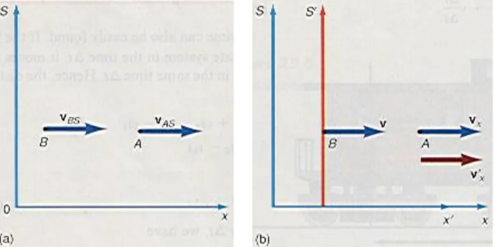
If there is more than one body in motion with respect to the stationary frame, the relative velocity between the two bodies is found by placing the S’ frame on one of the bodies in motion. That is, if body A is moving with a velocity vAS with respect to
the stationary frame S, and body B is moving with a velocity vBS, also with respect
to the stationary frame S, the velocity of A as observed from B, vAB, is simply
vAB = vAS vBS (1.11)
as seen in figure 1.7(a).
Figure 1.7 Relative velocities.
If we place the moving frame of reference S’ on body B, as in figure 1.7(b), then vBS = v, the velocity of the S’ frame. The velocity of the body A with respect to
S, vAS, is now set equal to vx, the velocity of the body with respect to the S frame.
The relative velocity of body A with respect to body B, vAB, is now v’x, the velocity of
the body with respect to the moving frame of reference S’. Hence the velocity v’x of
the moving body with respect to the moving frame is determined from equation 1.11 as
v’x = vx v (1.12)
Note that equation 1.12 is the inverse of equation 1.10.
Example 1.3
Relative velocity. A car is traveling at a velocity of 95.0 km/hr to the right, with respect to a telephone pole. A truck, which is behind the car, is also moving to the right at 65.0 km/hr with respect to the same telephone pole. Find the relative velocity of the car with respect to the truck.
We represent the telephone pole as the stationary frame of reference S, while we place the moving frame of reference S’ on the truck that is moving at a speed v = 65.0 km/hr. The auto is moving at the speed v = 95.0 km/hr with respect to S. The velocity of the auto with respect to the truck (or S’ frame) is v’x and is found from
equation 1.12 as
v’x = vx v
= 95.0 km/hr 65.0 km/hr = 30.0 km/hr
The relative velocity is +30.0 km/hr. This means that the auto is pulling away or separating from the truck at the rate of 30.0 km/hr. If the auto were moving toward the S observer instead of away, then the auto’s velocity with respect to S’ would have been
v’x = vx v = 95.0 km/hr 65.0 km/hr
= 160.0 km/hr
That is, the truck would then observe the auto approaching at a closing speed of
160 km/hr. Note that when the relative velocity v’x is positive the two moving
objects are separating, whereas when v’x is negative the two objects are closing or
coming toward each other.
Go to Interactive Example
To complete the velocity transformation equations, we use the fact that y = y’ and z = z’, thereby giving us
v’y = dy’ = dy = vy (1.13)
dtdt and
v’z = dz’ = dz = vz (1.14)
dt dt
The Galilean transformations of velocities can be summarized as:
vx = v’x + v (1.10)
v’x = vx v (1.12)
v’y = vy (1.13)
1.3 The Invariance of the Mechanical Laws of Physics
under a Galilean Transformation
Although the velocity of a moving object is different when observed from a stationary frame rather than a moving frame of reference, the acceleration of the body is the same in either reference frame. To see this, let us start with equation 1.12,
v’x = vx v
The change in each term with time is
dv’x = dvx dv (1.15)
dt dt dt
But v is the speed of the moving frame, which is a constant and does not change with time. Hence, dv/dt = 0. The term dv’x/dt = a’x is the acceleration of the body
with respect to the moving frame, whereas dvx/dt = ax is the acceleration of the body
with respect to the stationary frame. Therefore, equation 1.15 becomes
a’x = ax (1.16)
Equation 1.16 says that the acceleration of a moving body is invariant under a Galilean transformation. The word invariant when applied to a physical quantity means that the quantity remains a constant. We say that the acceleration is an invariant quantity. This means that either the moving or stationary observer would measure the same numerical value for the acceleration of the body.
If we multiply both sides of equation 1.16 by m, we get
ma’x = max (1.17)
But the product of the mass and the acceleration is equal to the force F, by Newton’s second law. Hence,
F’ = F (1.18) Thus, Newton’s second law is also invariant to a Galilean transformation and applies to all inertial observers.
The laws of conservation of momentum and conservation of energy are also invariant under a Galilean transformation. We can see this for the case of the perfectly elastic collision illustrated in figure 1.8. We can write the law of conservation of momentum for the collision, as observed in the S frame, as
m1v1 + m2v2 = m1V1 + m2V2 (1.19)
the collision, V1 is the velocity of ball 1 after the collision, and V2 is the velocity of ball 2 after the collision. But the relation between the velocity in the S and S’ frames, found from equation 1.11 and figure 1.8, is
Figure 1.8 A perfectly elastic collision as seen from two inertial frames.
' 1 1 ' 2 2 ' 1 1 ' 2 2 v v v v v v V V v V V v (1.20)
Substituting equations 1.20 into equation 1.19 for the law of conservation of momentum yields
m1v’1 + m2v’2 = m1V’1 + m2V’2 (1.21) Equation 1.21 is the law of conservation of momentum as observed from the moving S’ frame. Note that it is of the same form as the law of conservation of momentum as observed from the S or stationary frame of reference. Thus, the law of conservation of momentum is invariant to a Galilean transformation.
The law of conservation of energy for the perfectly elastic collision of figure 1.8 as viewed from the S frame is
1 m1v12 + 1 m2v22 = 1 m1V12 + 1 m2V22 (1.22) 2 2 2 2
By replacing the velocities in equation 1.22 by their Galilean counterparts, equation 1.20, and after much algebra we find that
1 m1v1’ 2 + 1 m2v2’ 2 = 1 m1V1’ 2 + 1 m2V2’ 2 (1.23) 2 2 2 2
Equation 1.23 is the law of conservation of energy as observed by an observer in the moving S’ frame of reference. Note again that the form of the equation is the same as in the stationary frame, and hence, the law of conservation of energy is invariant to a Galilean transformation. If we continued in this manner we would prove that all the laws of mechanics are invariant to a Galilean transformation.
1.4 Electromagnetism and the Ether
We have just seen that the laws of mechanics are invariant to a Galilean transformation. Are the laws of electromagnetism also invariant?
Consider a spherical electromagnetic wave propagating with a speed c with respect to a stationary frame of reference, as shown in figure 1.9. The speed of this
Figure 1.9 A spherical electromagnetic wave. electromagnetic wave is
c = r t
where r is the distance from the source of the wave to the spherical wave front. We can rewrite this as
r = ct or
or
r2 c2t2 = 0 (1.24) The radius r of the spherical wave is
r2 = x2 + y2 + z2 Substituting this into equation 1.24, gives
x2 + y2 + z2 c2t2 = 0 (1.25) for the light wave as observed in the S frame of reference. Let us now assume that another observer, moving at the speed v in a moving frame of reference S’ also observes this same light wave. The S’ observer observes the coordinates x’ and t’, which are related to the x and t coordinates by the Galilean transformation equations as
x = x’ + vt (1.1) y = y’ (1.2) z = z’ (1.3) t = t’ (1.4) Substituting these Galilean transformations into equation 1.25 gives
(x’ + vt)2 + y’ 2 + z’ 2 c2t’ 2 = 0 x’ 2 + 2x’vt + v2t2 + y’ 2 + z’ 2 c2t’ 2 = 0 or
x’ 2 + y’ 2 + z’ 2 c2t’ 2 = 2x'vt v2t2 (1.26) Notice that the form of the equation is not invariant to a Galilean transformation. That is, equation 1.26, the velocity of the light wave as observed in the S’ frame, has a different form than equation 1.25, the velocity of light in the S frame. Something is very wrong either with the equations of electromagnetism or with the Galilean transformations. Einstein was so filled with the beauty of the unifying effects of Maxwell’s equations of electromagnetism that he felt that there must be something wrong with the Galilean transformation and hence, a new transformation law was required.
A further difficulty associated with the electromagnetic waves of Maxwell was the medium in which these waves propagated. Recall from your general physics course, that a wave is a disturbance that propagates through a medium. When a rock, the disturbance, is dropped into a pond, a wave propagates through the water, the medium. Associated with a transverse wave on a string is the motion of the particles of the string executing simple harmonic motion perpendicular to the direction of the wave propagation. In this case, the medium is the particles of the string. A sound wave in air is a disturbance propagated through the medium air. In fact, when we say that a sound wave propagates through the air with a velocity of
A sound wave in water propagates through the water while a sound wave in a solid propagates through the solid. The one thing that all of these waves have in common is that they are all propagated through some medium. Classical physicists then naturally asked, “Through what medium does light propagate?” According to everything that was known in the field of physics in the nineteenth century, a wave must propagate through some medium. Therefore, it was reasonable to expect that a light wave, like any other wave, must propagate through some medium. This medium was called the luminiferous ether or just ether for short. It was assumed that this ether filled all of space, the inside of all material bodies, and was responsible for the transmission of all electromagnetic vibrations. Maxwell assumed that his electromagnetic waves propagated through this ether at the speed c = 3 108 m/s.
An additional reason for the assumption of the existence of the ether was the phenomena of interference and diffraction of light that implied that light must be a wave. If light is an electromagnetic wave, then it is waving through the medium called ether.
There are, however, two disturbing characteristics of this ether. First, the ether had to have some very strange properties. The ether had to be very strong or rigid in order to support the extremely large speed of light. Recall from your general physics course that the speed of sound at 0 C is 330 m/s in air, 1520 m/s in water, and 3420 m/s in iron. Thus, the more rigid the medium the higher the velocity of the wave. Similarly, for a transverse wave on a taut string the speed of propagation is / T v m l
where T is the tension in the string. The greater the value of T, the greater the value of the speed of propagation. Greater tension in the string implies a more rigid string. Although a light wave is neither a sound wave nor a wave on a string, it is reasonable to assume that the ether, being a medium for propagation of an electromagnetic wave, should also be quite rigid in order to support the enormous speed of 3 108 m/s. Yet the earth moves through this rigid medium at an orbital speed of 3 104 m/s and its motion is not impeded one iota by this rigid medium. This is very strange indeed.
The second disturbing characteristic of this ether hypothesis is that if electromagnetic waves always move at a speed c with respect to the ether, then maybe the ether constitutes an absolute frame of reference that we have not been able to find up to now. Newton postulated an absolute space and an absolute time in his Principia: “Absolute space, in its own nature without regard to anything external remains always similar and immovable.” And, “Absolute, true, and mathematical time, of itself and from its own nature flows equally without regard to anything external.” Could the ether be the framework of absolute space? In order to settle these apparent inconsistencies, it became necessary to detect this medium, called the ether, and thus verify its very existence. Maxwell suggested a crucial
experiment to detect this ether. The experiment was performed by A. A. Michelson and E. E. Morley and is described in section 1.5.
1.5 The Michelson-Morley Experiment
If there is a medium called the ether that pervades all of space then the earth must be moving through this ether as it moves in its orbital motion about the sun. From the point of view of an observer on the earth the ether must flow past the earth, that is, it must appear that the earth is afloat in an ether current. The ether current concept allows us to consider an analogy of a boat in a river current.
Consider a boat in a river, L meters wide, where the speed of the river current is some unknown quantity v, as shown in figure 1.10. The boat is capable
Figure 1.10 Current flowing in a river.
of moving at a speed V with respect to the water. The captain would like to measure the river current v, using only his stopwatch and the speed of his boat with respect to the water. After some thought the captain proceeds as follows. He can measure the time it takes for his boat to go straight across the river and return. But if he heads straight across the river, the current pushes the boat downstream. Therefore, he heads the boat upstream at an angle such that one component of the boat’s velocity with respect to the water is equal and opposite to the velocity of the current downstream. Hence, the boat moves directly across the river at a velocity V’, as shown in the figure. The speed V’ can be found from the application of the Pythagorean theorem to the velocity triangle of figure 1.10, namely
V2 = V’ 2 + v2 Solving for V’, we get
2 2
'
V V v
Factoring out a V, we obtain, for the speed of the boat across the river,
2 2
' 1 /
We find the time to cross the river by dividing the distance traveled by the boat by the boat’s speed, that is,
tacross = L V’ The time to return is the same, that is,
treturn = L V’ Hence, the total time to cross the river and return is
t1 = tacross + treturn = L + L = 2L V’ V’ V’ Substituting V’ from equation 1.27, the time becomes
1 2 2 2 1 / L t V v V
Hence, the time for the boat to cross the river and return is
1 2 2 2 / 1 / L V t v V (1.28)
The captain now tries another motion. He takes the boat out to the middle of the river and starts the boat downstream at the same speed V with respect to the water. After traveling a distance L downstream, the captain turns the boat around and travels the same distance L upstream to where he started from, as we can see in figure 1.10. The actual velocity of the boat downstream is found by use of the Galilean transformation as
V’ = V v Downstream while the actual velocity of the boat upstream is
V’ = V v Upstream
We find the time for the boat to go downstream by dividing the distance L by the velocity V’. Thus the time for the boat to go downstream, a distance L, and to return is
t2 = tdownstream + tupstream = L + L V + v V v
Finding a common denominator and simplifying, t2 = L(V v) + L(V v) (V v)(V v) = LV Lv + LV + Lv V 2 + vV vV v2 = 2LV V2 v2 = 2LV/V2 V 2/V 2 v2/V2 t2 = 2L/V (1.29) 1 v2/V 2
Hence, t2 in equation 1.29 is the time for the boat to go downstream and return. Note from equations 1.28 and 1.29 that the two travel times are not equal.
The ratio of t1, the time for the boat to cross the river and return, to t2, the time for the boat to go downstream and return, found from equations 1.28 and 1.29, is
2 2 1 2 2 2 2 / / 1 / 2 / / 1 / L V v V t t L V v V
2 2
2 2 1 / 1 / v V v V 2 2 1 2 1 / t v V t (1.30) Equation 1.30 says that if the speed v of the river current is known, then a relation between the times for the two different paths can be determined. On the other hand, if t1 and t2 are measured and the speed of the boat with respect to the water V is known, then the speed of the river current v can be determined. Thus, squaring equation 1.30, 2 2 1 2 2 2 1 t v t V 2 2 1 2 2 2 1 t v V t or 2 1 2 2 1 t v V t (1.31) Thus, by knowing the times for the boat to travel the two paths the speed of the river current v can be determined.Using the above analogy can help us to understand the experiment performed by Michelson and Morley to detect the ether current. The equipment used to measure the ether current was the Michelson interferometer and is sketched in figure 1.11. The interferometer sits in a laboratory on the earth. Because the earth moves through the ether, the observer in the laboratory sees an ether current moving past him with a speed of approximately v = 3.00 104 m/s,
Figure 1.11 The Michelson-Morley experiment.
the orbital velocity of the earth about the sun. The motion of the light throughout the interferometer is the same as the motion of the boat in the river current. Light from the extended source is split by the half-silvered mirror. Half the light follows the path OM1OE, which is perpendicular to the ether current. The rest follows the
path OM2OE, which is first in the direction of the ether current until it is reflected
from mirror M2, and is then in the direction that is opposite to the ether current. The time for the light to cross the ether current is found from equation 1.28, but with V the speed of the boat replaced by c, the speed of light. Thus,
1 2 2 2 / 1 / L c t v c
The time for the light to go downstream and upstream in the ether current is found from equation 1.29 but with V replaced by c. Thus,
t2 = 2L/c 1 v2/c2
The time difference between the two optical paths because of the ether current is
t = t2 t1
t = 2L/c 2L/c (1.32) 1 v2/c2 1v2/c2
To simplify this equation, we use the binomial theorem. That is,
(1 x)n = 1 nx + n(n 1)x2 n(n 1)(n 2)x3 + ... (1.33) 2! 3!
This is a valid series expansion for (1 x)n as long as x is less than 1. In this particular case,
x = v2 = (3.00 104 m/s)2 = 108 c2 (3.00 108 m/s)2
which is much less than 1. In fact, since x = 108, which is very small, it is possible to simplify the binomial theorem to
(1 x)n = 1 nx (1.34) That is, since x = 108, x2 = 1016, and x3 = 1024, the terms in x2 and x3 are negligible when compared to the value of x, and can be set equal to zero. Therefore, we can write the denominator of the first term in equation 1.32 as
1 2 2 2 2 2 2 2 2 1 1 1 ( 1) 1 1 / v v v v c c c c (1.35)
The denominator of the second term can be expressed as
1 1v2/c2 1 v2 c2 1/2 1 12 vc22 2 2 2 2 1 1 1 2 1 / v c v c (1.36)
Substituting equations 1.35 and 1.36 into equation 1.32, yields
2 2 2 2 2 1 2 1 1 2 L v L v t c c c c 2 2 2 2 2 1 1 1 2 L v v c c c 2 2 2 1 2 L v c c
The path difference d between rays OM1OE and OM2OE, corresponding to this time difference t, is
2 2 2 1 2 L v d c t c c c or d = Lv2 (1.37) c2
Equation 1.37 gives the path difference between the two light rays and would cause the rays of light to be out of phase with each other and should cause an interference fringe. However, as explained in your optics course, the mirrors M1 and M2 of the Michelson interferometer are not quite perpendicular to each other and we always get interference fringes. However, if the interferometer is rotated through 900, then the optical paths are interchanged. That is, the path that originally required a time t1 for the light to pass through, now requires a time t2 and vice versa. The new time difference between the paths, analogous to equation 1.32, becomes
t' = 2L/c 2L/c 1v2/c2 1 v2/c2 Using the binomial theorem again, we get
2 2 2 2 2 1 2 ' 1 1 2 L v L v t c c c c 2 2 2 2 2 1 1 1 2 L v v c c c 2 2 2 1 2 L v c c = Lv2 cc2
The difference in path corresponding to this time difference is
2 2 ' ' Lv d c t c cc or d’ = Lv2 c2
2 2 2 2 ' Lv Lv d d d c c d = 2Lv2 (1.38) c2
This change in the optical paths corresponds to a shifting of the interference fringes. That is,
d = n
or
n = d (1.39)
Using equations 1.38 for d, the number of fringes, n, that should move across the screen when the interferometer is rotated is
n = 2Lv2 (1.40)
c2
In the actual experimental set-up, the light path L was increased to 10.0 m by multiple reflections. The wavelength of light used was 500.0 nm. The ether current was assumed to be 3.00 104 m/s, the orbital speed of the earth around the sun. When all these values are placed into equation 1.40, the expected fringe shift is
n = 2(10.0 m)(3.00 104 m/s)2 (5.000 107 m)(3.00 108 m/s)2
= 0.400 fringes
That is, if there is an ether that pervades all space, the earth must be moving through it. This ether current should cause a fringe shift of 0.400 fringes in the rotated interferometer, however, no fringe shift whatsoever was found. It should be noted that the interferometer was capable of reading a shift much smaller than the 0.400 fringe expected.
On the rare possibility that the earth was moving at the same speed as the ether, the experiment was repeated six months later when the motion of the earth was in the opposite direction. Again, no fringe shift was observed. The ether cannot be detected. But if it cannot be detected there is no reason to even assume that it exists. Hence, the Michelson-Morley experiment’s null result implies that the all pervading medium called the ether simply does not exist. Therefore light, and all electromagnetic waves, are capable of propagating without the use of any medium. If there is no ether then the speed of the ether wind v is equal to zero. The null result of the experiment follows directly from equation 1.40 with v = 0.
equations with respect to the “fixed stars” still imply that the velocity of light along OM2 should be c v, where v is the earth’s orbital velocity, with respect to the fixed stars, and c is the velocity of light with respect to the source on the interferometer. Similarly, it should be c v along path M2O. But the negative result of the experiment requires the light to move at the same speed c whether the light was moving with the earth or against it. Hence, the negative result implies that the speed of light in free space is the same everywhere regardless of the motion of the source or the observer. This also implies that there is something wrong with the Galilean transformation, which gives us the c v and c v velocities. Thus, it would appear that a new transformation equation other than the Galilean transformation is necessary.
1.6 The Postulates of the Special Theory of Relativity
In 1905, Albert Einstein (1879-1955) formulated his Special or Restricted
Theory of Relativity in terms of two postulates.
Postulate 1: The laws of physics have the same form in all frames of reference moving at a constant velocity with respect to one another. This first postulate is sometimes also stated in the more succinct form: The laws of physics are invariant to a transformation between all inertial frames.
Postulate 2: The speed of light in free space has the same value for all observers, regardless of their state of motion.
Postulate 1 is, in a sense, a consequence of the fact that all inertial frames are equivalent. If the laws of physics were different in different frames of reference, then we could tell from the form of the equation used which frame we were in. In particular, we could tell whether we were at rest or moving. But the difference between rest and motion at a constant velocity cannot be detected. Therefore, the laws of physics must be the same in all inertial frames.
Postulate 2 says that the velocity of light is always the same independent of the velocity of the source or of the observer. This can be taken as an experimental fact deduced from the Michelson-Morley experiment. However, Einstein, when asked years later if he had been aware of the results of the Michelson-Morley experiment, replied that he was not sure if he had been. Einstein came on the second postulate from a different viewpoint. According to his first postulate, the laws of physics must be the same for all inertial observers. If the velocity of light is different for different observers, then the observer could tell whether he was at rest or in motion at some constant velocity, simply by determining the velocity of light in his frame of reference. If the observed velocity of light c’ were equal to c then the observer would be in the frame of reference that is at rest. If the observed velocity of light were c’ = c v, then the observer was in a frame of reference that was receding from the rest frame. Finally, if the observed velocity c’ = c v, then the observer would be in a frame of reference that was approaching the rest frame. Obviously