HAL Id: hal-02903854
https://hal.archives-ouvertes.fr/hal-02903854
Submitted on 21 Jul 2020
HAL is a multi-disciplinary open access
archive for the deposit and dissemination of
sci-entific research documents, whether they are
pub-lished or not. The documents may come from
teaching and research institutions in France or
abroad, or from public or private research centers.
L’archive ouverte pluridisciplinaire HAL, est
destinée au dépôt et à la diffusion de documents
scientifiques de niveau recherche, publiés ou non,
émanant des établissements d’enseignement et de
recherche français ou étrangers, des laboratoires
publics ou privés.
Distributed under a Creative Commons Attribution| 4.0 International License
S. Zhang, Annie Zavagno, J. Yuan, H. Liu, M. Figueira, D. Russeil, F.
Schuller, K. A. Marsh, Y. Wu
To cite this version:
S. Zhang, Annie Zavagno, J. Yuan, H. Liu, M. Figueira, et al.. H II regions and high-mass starless
clump candidates: I. Catalogs and properties. Astronomy and Astrophysics - A&A, EDP Sciences,
2020, 637, pp.A40. �10.1051/0004-6361/201936792�. �hal-02903854�
Astronomy
&
Astrophysics
https://doi.org/10.1051/0004-6361/201936792
© S. Zhang et al. 2020
H
II
regions and high-mass starless clump candidates
I. Catalogs and properties
?
,??
S. Zhang (
)
1, A. Zavagno
1,2, J. Yuan
3, H. Liu
4,5, M. Figueira
6, D. Russeil
1, F. Schuller
7,
K. A. Marsh
8, and Y. Wu
91Aix Marseille Univ., CNRS, CNES, LAM, Marseille, France
e-mail: siju.zhang@lam.fr
2Institut Universitaire de France (IUF), Paris, France
3National Astronomical Observatories, Chinese Academy of Sciences, 20A Datun Road, Chaoyang District, Beijing 100012,
PR China
4CASSACA, China-Chile Joint Center for Astronomy, Camino El Observatorio #1515, Las Condes, Santiago, Chile 5Departamento de Astronomía, Universidad de Concepción, Av. Esteban Iturra s/n, Distrito Universitario, 160-C, Chile 6National Centre for Nuclear Research, ul. Pasteura 7, 02-093, Warszawa, Poland
7Max-Planck-Institut für Radioastronomie, Auf dem Hügel 69, 53121 Bonn, Germany
8Infrared Processing and Analysis Center, California Institute of Technology, Pasadena, California 91125, USA 9Department of Astronomy, Peking University, 100871 Beijing, PR China
Received 26 September 2019 / Accepted 24 February 2020
ABSTRACT
Context. The role of ionization feedback on high-mass (>8 M ) star formation is still highly debated. Questions remain concerning the
presence of nearby HIIregions changes the properties of early high-mass star formation and whether HIIregions promote or inhibit the formation of high-mass stars.
Aims. To characterize the role of HIIregions on the formation of high-mass stars, we study the properties of a sample of candidates high-mass starless clumps (HMSCs), of which about 90% have masses larger than 100 M . These high-mass objects probably represent
the earliest stages of high-mass star formation; we search if (and how) their properties are modified by the presence of an HIIregion.
Methods. We took advantage of the recently published catalog of HMSC candidates. By cross matching the HMSCs and HIIregions,
we classified HMSCs into three categories: (1) the HMSCs associated with HIIregions both in the position in the projected plane
of the sky and in velocity; (2) HMSCs associated in the plane of the sky, but not in velocity; and (3) HMSCs far away from any HIIregions in the projected sky plane. We carried out comparisons between associated and nonassociated HMSCs based on statistical
analyses of multiwavelength data from infrared to radio.
Results. We show that there are systematic differences of the properties of HMSCs in different environments. Statistical analyses suggest that HMSCs associated with HIIregions are warmer, more luminous, more centrally-peaked and turbulent. We also clearly
show, for the first time, that the ratio of bolometric luminosity to envelope mass of HMSCs (L/M) could not be a reliable evolutionary probe for early massive star formation due to the external heating effects of the HIIregions.
Conclusions. We show HMSCs associated with HIIregions present statistically significant differences from HMSCs far away from HIIregions, especially for dust temperature and L/M. More centrally peaked and turbulent properties of HMSCs associated with HIIregions may promote the formation of high-mass stars by limiting fragmentation. High-resolution interferometric surveys toward HMSCs are crucial to reveal how HIIregions impact the star formation process inside HMSCs.
Key words. stars: formation – HIIregions – submillimeter: ISM
1. Introduction
The formation of high-mass (>8 M ) stars is still a mystery
as a consequence of their rapid evolution, larger distance, and violent feedback, which are all deeply embedded in molecular clouds. With the benefits of higher resolution and sensitiv-ity from millimeter interferometers such as Atacama Large Millimeter/Submillimeter Array (ALMA), the details happening at the very early evolutionary stages of high-mass star forma-tion (HMSF) have been investigated in recent years. Two popular models for HMSF have been discussed widely: (1) monolithic ?Full Table 4 and additional data are only available at the CDS
via anonymous ftp tocdsarc.u-strasbg.fr(130.79.128.5) or via http://cdsarc.u-strasbg.fr/viz-bin/cat/J/A+A/637/A40
??This publication is based on the SEDIGISM and PPMAP data.
collapse (McKee & Tan 2003;Krumholz et al. 2009; Csengeri et al. 2018; Sanna et al. 2019; Motogi et al. 2019) and (2) competitive accretion (Bonnell et al. 2007; Cyganowski et al. 2017;Fontani et al. 2018). It is possible that these models are not strongly and mutually incompatible as described by many current studies; these two models of HMSF are expected to be merged into a unified and consistent star formation model with the progress of observations and theories (Schilke 2015). The new evolutionary scenario proposed byMotte et al.(2018) suggests that the large-scale (0.1–1 pc) gas reservoirs, known as starless massive dense cores (MDCs) or starless clumps, could replace the high-mass analogs of prestellar cores (about 0.02 pc). These mass reservoirs could concentrate their mass into high-mass cores at the same time when stellar embryos are accreting.
A40, page 1 of26
The complexities of HMSF result from not only the contro-versially basic pictures of formation mechanism but also from the environmental impacts on the formation process. The pow-erful UV radiation of massive stars ionizes hydrogen to form HIIregions. Because high-mass stars form in the densest parts of
molecular clouds, HIIregions are expected to become a typical
environment of HMSF. Previous studies found that at least 30% of HMSF in the Galaxy are observed at the edges of HIIregions (Deharveng et al. 2010;Kendrew et al. 2016; Palmeirim et al. 2017).
The possible impacts of ionization radiation on star forma-tion have been investigated in many publicaforma-tions. H IIregions
could trigger star formation with several mechanisms, mainly depending on the density and configuration of the surround-ing medium (see Sect. 5 in Deharveng et al. 2010), such as the collect and collapse (C&C) mechanism in IR dust bubbles (Zavagno et al. 2010; Samal et al. 2014; Duronea et al. 2017) or the radiation-driven implosion (RDI) mechanism in pillars or bright rimmed clouds (Bertoldi 1989;Imai et al. 2017;Marshall & Kerton 2019).
The interferometric studies of HMSF generally focus on physical and/or chemical phenomena inside the massive clumps or in a single field of view. This could produce a blind zone for the possible interactions between massive clumps, HMSF, and their various environments. For example,Csengeri et al.(2017a) used ALMA to survey fragmentation at the early evolutionary stage of IR-quiet massive clumps and ignored possible environ-mental factors, even though environenviron-mental factors such as the presence of nearby HIIregion could impact the fragmentation
process (Busquet et al. 2016).
In a series of forthcoming papers, we try to systematically explore how the environment of the HIIregion changes HMSF,
particularly for the HMSF at the very early evolutionary stages. High-mass starless clumps (HMSCs), which are very cold (dust temperature of around 10 to 20 K) and massive (from a few hundreds to several thousands of solar mass at a typical scale of 0.1–1 pc), are thought to be the possible precursors of high-mass stars. These sources are likely at the earliest stage of HMSF (quiescent prestellar stage), and only less than 10% of the clumps with the ability to probably form massive stars are at this stage, indicating their short lifetime (Urquhart et al. 2018). Observa-tionally, HMSCs are dark against their background environment from optical to mid-infrared (mid-IR) owing to the absence of the embedded protostellar objects.
Systematic studies of HMSCs under the effect of HIIregions
are very crucial to characterize the influence of the HIIregions
and how the influence impacts very early HMSF and the asso-ciated gas dynamics. We investigate the impacts of HIIregions
on a large sample of 463 HMSC candidates recently selected by Yuan et al.(2017) (written briefly as Y17 in the following) in the inner Galactic plane. As in the first paper, we cross match HMSCs and HIIregions based on their mutual correlation in the
plane of sky to ascertain their association and then investigate the differences of the physical properties between the HMSCs associated with and those not associated with HIIregions.
This paper is organized as follows: the sample selection and archival data acquisition are described in Sect. 2. Section 3
shows how we determine the basic parameters of HMSCs with updated data, followed by cross matching of H II regions and
HMSCs in Sect. 4. In Sects.5–8, we explore and compare the properties of different HMSCs. In Sect.9, we discuss the results to shed light on the role of ionization feedback on modifying the physical properties of HMSCs. The conclusions are finally presented in Sect.10.
Table 1. Star formation indicators.
Search IR point sources Maser Others S16 Hi-GAL 70 µm H2O masers UCHIIregions
2–24 µm YSOs CH3OH masers
Y17
Hi-GAL 70 µm Masers(a) HIIregions
MIPSGAL sources extended 24 µm
GLIMPSE YSOs cm radio sources
IR sources HH objects
YSOs (C.)(b) outflows (C.)
PMS (C.) T Tau (C.) HAEBE (C.)
Notes. (a)The sources in bold are the star formation indicators in
SIMBAD database.(b)The abbreviation “C.” means candidate.
2. Sample and data
2.1. Sample of HMSC candidates
There are several studies dedicated to the search of starless clumps in the Milky Way.Elia et al.(2017) explore the physical properties of Herschel infrared Galactic Plane Survey (Hi-GAL, seeMolinari et al. 2010) compact sources in the inner Galaxy and termed the starless cores or clumps when they are not asso-ciated with 70 µm counterpart. A large number of 76338 starless clump/core candidates are found. About 65, 52, and 3% of these clumps are compatible with massive star formation according to the different thresholds, which are M(r) > 870 M (r/pc)1.33,
or Σcrit = 0.2 and 1 g cm−2 suggested byKauffmann & Pillai
(2010),Butler & Tan(2012), and Krumholz & McKee(2008), respectively. With Bolocam Galactic Plane Survey data (BGPS;
Aguirre et al. 2011),Svoboda et al.(2016) (S16) obtained a sam-ple of 2223 starless clump candidates in 10◦ < l < 65◦ based
on the absence of a series of observational signatures of star formation (see Table1).
The recent search for starless clumps by Y17, which targeted at only massive starless clumps (&100 M for 90% of these
clumps at a typical scale of 0.2–0.8 pc) in the inner Galactic plane (|l| < 60◦, |b| < 1◦), resulted in a sample of 463 HMSC
candidates by extracting APEX Telescope Large Area Survey of the Galaxy 870 µm clumps (ATLASGAL; Csengeri et al. 2014) based on a series of selection criteria. Firstly, Y17 selected clumps with a 870 µm peak intensity higher than 0.5 Jy beam−1
to ensure that the column density is sufficient to form a massive star. Then, these authors removed clumps with star formation indicators such as young stellar objects (YSOs) identified by Galactic Legacy Infrared Midplane Survey Extraordinaire data (GLIMPSE;Churchwell et al. 2009), MIPS Galactic Plane Sur-vey 24 µm data (MIPSGAL; Carey et al. 2009), and Herschel 70 µm data (Molinari et al. 2010). Besides, various kinds of star formation indicators in the SIMBAD database1 were also used.
Finally, all candidates were inspected in Spitzer images by eye. A comparison between the samples of Y17 and S16 shows that only 20% of ATLASGAL counterparts of BGPS starless clumps are in the HMSC sample of Y17. This could be due to denser or more reliably starless properties of HMSCs in the sample of Y17. Additional star formation indicators such as out-flows (candidates) are considered. Furthermore, the inclusion
1 http://simbad.u-strasbg.fr/simbad/sim-display?data=
of extended 24 µm could mitigate false identifications due to a strong background. Another factor could be the better reso-lution of ATLASGAL (about 2000) compared to BGPS (about
3300), which may resolve one BGPS clump to more individual
structures in ATLASGAL considering that BGPS could detect the similar mass range as ATLASGAL (Ellsworth-Bowers et al. 2015).
We chose the sample by Y17 as our HMSC candidates because it is probably more robust and focused on massive clumps. Even though a larger number of star formation indi-cators are cross matched, the selected HMSCs are still starless candidates rather than absolutely starless (Pillai et al. 2019). One of the examples is the massive 70 µm quiet clump, which was considered a more reliable starless candidate in previous, while evidences of embedded low- to intermediate-mass star formation have been found in such clump recently (Traficante et al. 2017;
Svoboda et al. 2019;Li et al. 2019;Sanhueza et al. 2019). Basi-cally, HMSCs hereafter represent HMSC candidates unless there are special explanations.
2.2. Ionized region sample
The ionized regions created during HMSF produce a shell or layer of photodissociation region (PDR) that can be observed by the PAH2 emission in the mid-IR, for example, via GLIMPSE
8 µm or Wide-field Infrared Survey Explorer 12 µm emission (WISE;Wright et al. 2010). This shell or layer surrounds the hot thermal dust emission of ionized regions, which can be observed in MIPSGAL 24 µm or WISE 22 µm emission. The photodisso-ciation shell and the inner hot thermal dust emission in mid-IR images make up the objects that are generally named as IR dust bubbles (Deharveng et al. 2010).
The ionized regions are originally traced by the emission from ionized gas such as the free-free centimeter continuum or radio recombination lines (RRL). The close correlations between the mid-IR hot dust emission and the centimeter radio free–free emission of H II regions have been revealed by several
stud-ies (Ingallinera et al. 2014;Makai et al. 2017), which indicate a tight spatial association between H II regions and IR dust
bubbles.Churchwell et al.(2006) cataloged 322 IR bubbles by visual examination of GLIMPSE mid-IR images. These authors argued that most of the bubbles are formed by hot young stars in HMSF regions. Only three of their bubbles are identified as known supernova remnants (SNRs). The overlapping fraction between HIIregions and bubbles could approach '85% or even
more in other similar studies (Deharveng et al. 2010;Bania et al. 2010;Anderson et al. 2011), which shed light on the association between HIIregions, bubbles, and HMSF.
We used the IR bubbles identified in mid-IR images as our candidates of HIIregions. Based on GLIMPSE images, a large
catalog of more than 5000 IR bubbles is attained through the visual identification by tens of thousands citizens within Milky Way Project (MWP) (Simpson et al. 2012;Kendrew et al. 2012). This catalog consists of the following two types of bubbles based on angular size: large (>3000) and small (<3000) bubbles.
In this work, we take advantage of the sample of 3744 large bubbles as our H II region candidates. The small bubble
can-didates are ignored because of their high level of confusion with other astronomical objects unrelated to star formation such as AGB. Another reason is that the resolutions of millimeter and far-infrared (far-IR) images in our studies are close to the scale of 2 Polycyclic aromatic hydrocarbon (PAH) commonly exits in the PDR
(Fleming et al. 2010).
small bubble (2000–3000). The unresolved HIIregions could mix
with nearby HMSCs, leading to the unreal properties of HMSCs. In addition,Anderson et al.(2014) constructed a catalog of over 8000 Galactic H II regions (candidates), around 2000 of
which are known HIIregions. They developed an online tool for viewing WISE emission of these HIIregions3, which is updated
when there are new radio continuum and RRL observations such as HIIRegion Discovery Survey (HRDS) (Anderson et al. 2015, 2018;Wenger et al. 2019). The distant Galactic HIIregions are
also included in HRDS (Anderson et al. 2015).Anderson et al.
(2014) propose that WISE has a sensitivity to detect all Galactic H IIregions (see Fig. 2 in their paper). The size and position of H II region (bubble) candidates in this online tool are
out-lined by characteristic morphology of WISE mid-IR emission. We use this catalog and associated online tool as supplements in searching for our HIIregion candidates.
2.3. Survey data
The main observing parameters of the surveys we used for this work are listed in Table 2. Several types of data are included as follows: (1) infrared data: GLIMPSE mapped the Galactic plane in mid-IR and we used this survey to show the spatial dis-tribution of PAH, hot dust, and YSOs. (2) (Sub)millimeter and far-IR continuum data: ATLASGAL 870 µm survey (|l| < 60◦,
|b| < 1.5◦) and Point Process Mapping for Hi-GAL (Hi-GAL
PPMAP;Marsh et al. 2015) column density and dust tempera-ture data are used. A more detailed description about Hi-GAL PPMAP is given in Sect.3.3. (3) (Sub)millimeter molecular line data: Structure, Excitation, and Dynamics of the Inner Galactic InterStellar Medium survey (SEDIGISM;Schuller et al. 2017) mapped the inner Galactic plane (−60◦ ≤ l ≤ 18◦, |b| ≤ 0.5◦) in
the J = 2−1 rotational transition of 13CO and C18O using the
SHFI instrument on APEX with a spatial resolution of about 3000 and a velocity resolution of 0.25 km s−1 (Schuller et al. 2017). We used this survey to explore kinematics of the HMSCs. The survey is described in more detail in Sect.8. (4) Centime-ter radio images: Multi-Array Galactic Plane Imaging Survey (MAGPIS, first quadrant the Galactic plane;Helfand et al. 2006), Sydney University Molonglo Sky Survey (SUMSS, southern
sky;Bock et al. 1999), and VLA Galactic Plane Survey (VGPS,
18◦ < l < 67◦and b < 1.3◦ to 3.3◦;Stil et al. 2006) are used to
indicate the HIIregions.
3. Physical parameters
3.1. Velocity and distance
A reliable velocity determination is crucial to estimate a reliable set of other physical properties of the clumps. We take advan-tage of the results of velocity component identification from the Hi-GAL distance project (Mege et al., in prep.) to revise the systematic velocity (vlsr) estimated by Y17. This project aims
to determine the vlsr and distance of about 150 000
Hi-GAL-selected compact sources as accurately as possible by using all the molecular tracers available for the sources. In practice, we determine the most reliable vlsrof a clump by carefully inspecting
the spatial association and morphology between dust and molec-ular line emission. The velocity component with a morphology most similar to ATLASGAL emission of the HMSCs is selected. An example of the velocity determination of the HMSCs with the results of Hi-GAL distance project is shown in Fig.1.
Table 2. Information about the surveys used in this work.
Survey Band Resolutions Pixel sizes Facilities References
GLIMPSE
3.6 µm
'200 1.200 Spitzer IRAC Churchwell et al.(2009)
4.5 µm 5.8 µm 8.0 µm
ATLASGAL 870 µm 19.200 600 APEX LABOCA Schuller et al.(2009)
SEDIGISM 220 GHz 3000 9.500 APEX SHFI Schuller et al.(2017)
PPMAP – 1200 600 Herschel Marsh et al.(2015)
MAGPIS 6 cm 1.8
00 0.600
VLA Helfand et al.(2006)
21 cm 6.000 200
90 cm 2500 600
SUMSS 35 cm 4300× 4300cosec|δ| 1100 MOST Bock et al.(1999)
VGPS 20 cm 4500 1800 VLA Stil et al.(2006)
(a) (b) (c) (d) −200 −150 −100 −50 0 50 100 150 200 Velocity (km/s) 0 2 4 6 8 10 12 In tensit y (K) (e) 13CO J = 2-1
Fig. 1.Example of the vlsrdetermination with the results of Hi-GAL
dis-tance project for the HMSC G305.1543+0.0477. Panel a: ATLASGAL contours overlaid on RGB image constructed from GLIMPSE 24 µm (in red), 8 µm (in green), and 4.5 µm (in blue) images. Panels b–d: SEDIGISM13CO J = 2−1 intensity at the velocity of −48.15, −36.47,
and −29.08 km s−1, respectively. Black ellipses indicate the size and
position of the HMSCs taken from Y17. Gray ellipses indicate the clumps identified in the corresponding intensity maps of the Hi-GAL distance project. Gray and red solid lines in (e) indicate the vlsr
com-ponents identified with 13CO J = 2−1 spectra of the HMSC by the
Hi-GAL distance project. The red lines highlight the vlsr for the
cor-responding intensity maps (b), (c), and (d). According to the mapping results, the most proper vlsrfor the clump is −36.47 km s−1.
After revising the velocity, we used the same methods as that adopted in Y17 to derive the distance from renewed veloc-ity, which is a parallax-based distance estimator developed by
Reid et al. (2016) based on the Bayesian maximum-likelihood
approach. We carefully considered kinematic distance ambigui-ties (KDA) when determining the distance. We applied the KDA solution results ofUrquhart et al.(2018) to ascertain the distance. If the HMSCs are not included in Urquhart et al. (2018), we followed their work flows to solve the ambiguities, which use a series of evidence such as the scale height of the Galactic plane, H I self-absorption (H I SA), and extinction (IR dark
clouds). More detailed information about KDA solutions is given in AppendixA.
3.2. Kinematic uncertainty
The renewed vlsrand its comparisons with that in Y17 are shown
in Fig. 2. Most of the HMSCs except for the low-longitude sources are located at or close to spiral arms as shown in Fig.2a. The HMSCs toward the Galactic center have a radial component of the velocity that is only a small fraction of the entire velocity of the clump, making the rotation curve and resulted kinematic distance are just not reliable. Using any kinematic information in extremely low longitude is challenging, as shown by the sig-nificant l − vlsr structure blending in |l| < 3◦ region in Fig.2a.
Furthermore, the commonly existing broad line width (several dozens of km s−1) of molecular lines in this region increases
the difficulties to identify a proper vlsr (Kruijssen et al. 2015; Ginsburg et al. 2016). The 90th percentiles of the identified vlsr difference between Y17 and this paper are 3.9 km s−1 and
64.6 km s−1 for |l| > 3◦ and |l| ≤ 3◦, respectively. This shows
the large uncertainty in vlsr identification for low-longitude
clumps.
The strong radial streaming motions caused by the Galactic bar, which could also impact the l − vlsr structure, are carefully
considered byEllsworth-Bowers et al.(2015). Figure2a shows that only few HMSCs are located in the exclusion regions pro-posed byEllsworth-Bowers et al.(2015) and that these HMSCs are close to the boundaries of exclusion regions. Thus, this kind of uncertainty is not dominating for our HMSCs. Considering the unreliable velocity and kinematic distance in lower longi-tude, we exclude a total of 125 HMSCs located in |l| ≤ 3◦ from
−60 −40 −20 0 20 40 60
Galactic Longitude (deg) −150 −100 −50 0 50 100 150 ∆v lsr (km s − 1) (b) |∆| ≥ 90th percentile |∆| < 90th percentile −150 −100 −50 0 50 100 150 vlsr (km s − 1) (a) Near 3 kpc arm Perseus Norma Sagittarius Scutum-Centaurius
Fig. 2. New HMSC vlsr (this work) and those in Y17. Panels a and
b: renewed vlsr and difference between renewed vlsr and those in Y17,
∆vlsr = vlsrnew− vlsrY17, respectively. The 90th percentile of |∆vlsr| for
HMSCs located at higher longitude (|l| > 3◦) is 3.9 km s−1, shown as
red dashed lines in (b). The red and black dots represent HMSCs with |∆vlsr| values larger and smaller than 3.9 km s−1, respectively. The gray
region indicates the lower-longitude region, |l| < 3◦, where the HMSCs
are excluded from following analyses. Orange regions are considered
byEllsworth-Bowers et al.(2015). The four spiral and local arms are
shown by different colors and their positions are taken fromUrquhart
et al.(2018) and its referencesTaylor & Cordes(1993) andBronfman
et al.(2000). Most of the errors of vlsrare less than 2 km s−1and the
associated error bars are smaller than the point size in (a).
The uncertain kinematics is not the only reason to exclude the lower-longitude HMSCs. Possible different star formation mechanism and history compared to other molecular cloud– star formation complexes are also possible reasons. The central molecular zone (CMZ) is about 400 pc in size (angular scale at the distance of the Earth is about 0.4/8.34 rad '3◦). The
star formation rate (SFR) in the CMZ is an order of magnitude lower than expected (Lu et al. 2019). One of the explanations for the low SFR is that the clouds in CMZ are without active star formation at very early evolutionary stages because of the co-impacts of high turbulence, magnetic field, and a number of other processes (Kruijssen et al. 2014). A higher density is needed for the collapse of the clumps in the CMZ. Therefore, the inhibited HMSF could result in the overproduction of HMSCs (26% HMSCs are in the region |l| < 3◦). Our study focuses on
the impacts of HIIregions on HMSCs, thus it is more reliable
to only use the higher-longitude HMSCs, which could avoid the complex co-impacts in CMZ.
The 70th percentile of the distance difference |∆D| between
this paper and Y17 is about 0.8 kpc, which is shown in Fig.3a in red dashed lines. Owing to the small |∆vlsr| for most HMSCs,
the improvement in solving KDA problem could be the most possible reason for the large difference between our new dis-tance determination and those in Y17. For HMSCs with a similar vlsr but large |∆D|, their |∆D| are approximately equal
to the differences between far and near distance Dfar− Dnear
in KDA solutions, as shown in Fig.3b; this suggests the large |∆D| are mainly due to the difference of KDA solutions. Nearly
70 HMSCs in total have a different KDA solution compared to those in Y17. −60 −40 −20 0 20 40 60
Galactic Longitude (deg) −10 0 10 ∆D (kp c) (a). ∆D= Dnew− DY 17 Non IR Dark HISA Tangent Scale height Literature 2 4 6 8 10 12 14 |∆D| (kpc) 10−1 100 101 (D f ar − Dnear )/ |∆ D | (b). KDA & ∆D
Fig. 3.New distance of HMSC (this work) and those in Y17. Panel a:
distance difference ∆D = Dnew− DY17. The red dashed lines show
|∆D| = 0.8 kpc, representing the 70th percentile of |∆D|. The red, blue,
orange, green, and purple dots mean that their KDA are solved by IR dark, H ISA, tangent, scale height, and literature, respectively (see Table4and AppendixA). The black dots are the sources without KDA solution. Panel b: |∆D| and its relation with the difference between
resulted far distance and near distance Dfar− Dnear. Only HMSCs with
|∆D| > 0.8 kpc and |∆vlsr| < 3.9 km s−1are shown. The gray region shows
(Dfar− Dnear)/|∆D| = 1 ± 0.8/|∆D|, indicating the error of relation. The
gray cross shows the typical error.
3.3. Column density and dust temperature
One of the classical ways to investigate the dust properties of HMSC is to combine far-IR to millimeter multiwavelength data and then fit the spectral energy distribution (SED) pixel by pixel. All images need to be smoothed to the largest beam size in the data set and then fitted with the modified blackbody function at each pixel. Principally, we made use of the H2 column
den-sity (NH2) and dust temperature (Tdust) resulting from the Y17
SED fitting to update the physical properties according to the renewed distance. Besides, we also utilized the higher resolu-tion PPMAP Hi-GAL data set in investigaresolu-tions of density and temperature profile.
3.3.1. Results from Y17
In Y17, the Hi-GAL 160, 250, 350, 500 µm, and ATLAS-GAL 870 µm images are smoothed to the largest beam of the data set, which is 36.400. After carefully removing the
fore-ground/background flux, gray-body functions are fitted pixel-by-pixel with a dust opacity of κν =3.33(ν/600GHz)β cm2g−1
and an emissivity index of β = 2. In this paper, physical proper-ties (e.g., clump mass Mclump, number density nH2, and size rpc)
are basically taken from Y17 but revised according to the new distance determination.
3.3.2. Higher resolution results from PPMAP
To explore the density/temperature structures of HMSCs, data with higher resolution is helpful because HMSF regions are
generally located at a distance farther than low mass star for-mation regions. To avoid degrading resolution when performing fitting process, Marsh et al. (2015) fit the SED based on the nonhierarchical Bayesian procedure point process mapping tech-nique to utilize full instrumental point source functions (PSF).
Marsh et al.(2017) applied the PPMAP technique on the Hi-GAL 70, 160, 250, 350, and 500 µm images to get a series of Tdust–
differential NH2 planes, which means the column densities are
equally spaced in log space between 8 and 50 K and the dust temperature is the third dimension of NH2 maps (data cube).
The spatial resolution of the resulting PPMAP Hi-GAL NH2and
Tdustimages is 1200; the value is better than that from the
conser-vative SED fitting for Hi-GAL images ('3600). The typical errors
in the resulting NH2and Tdustare around 10–50% and around 1 K,
respectively.
Comparisons between PPMAP Hi-GAL Tdust and NH2 with
those in Y17 are shown in Fig.4. Generally, the PPMAP Hi-GAL Tdust value is a higher of 2–3 K than the value obtained in Y17.
At the low – Tdustend (<14 K for Tdustof Y17), the difference can
reach 5–7 K. The most likely reason for that is the difference in the wavelength of the data used because similar dust opacity and graybody functions are used by PPMAP and Y17. Y17 excluded Hi-GAL 70 µm emission and used additional 870 µm data to fit the SED, which could better constrain the shape of the SED at the long-wavelength end and lead to trace more the coldest parts of the clumps. Besides, Y17 carefully excluded the fore-ground/background flux when fitting the SED while this is not included in PPMAP Hi-GAL SED fitting.
When the data used in fitting are the same, the PPMAP tech-nique could provide a more accurate estimation of NH2and Tdust,
especially for the maximum of NH2, minimum of Tdust of the
clump (Marsh & Whitworth 2019). Even PPMAP Hi-GAL data should detect more compact structures than Y17 because of the higher resolution of the images; Fig.4shows that clumps NH2are
normally underestimated while Tdust are overestimated at the
low – Tdust end compared to Y17. This suggests that the errors
created during the SED-fitting process are dominated by the dif-ferent wavelength data used rather than difdif-ferent techniques or resolutions in our cases.
Considering these factors, we only used PPMAP data to esti-mate the column density/temperature structures (see details in Sect.7) rather than using these data to derive other global prop-erties of HMSCs such as NH2, Tdust, and the ratio of bolometric
luminosity to envelope mass L/M.
4. HIIregion cross matching
4.1. Criteria
To explore differences between HMSCs associated with and nonassociated with H II regions, we set two main criteria to
ascertain the association relationship.
The first criterion is the position in the plane of the sky.
Thompson et al. (2012) studied Red MSX Sources (RMSs;
see Lumsden et al. 2013) YSOs, and Ultra Compact (UC)
H II regions, which are regarded as the signatures of HMSF,
around 322 Spitzer mid-IR bubbles. With an angular cross-correlation function of RMSs and bubbles, these authors reveal that the location with the highest probability to find RMSs YSOs is around the effective radius Reffof the bubble. Furthermore, the
RMSs are essentially uncorrelated with bubbles and appear as field RMSs when the separations are larger than 2Reff. A similar
relationship for cold clumps has also been found in the MWP bubbles (Kendrew et al. 2016). If our HMSCs are precursors of
1021 1022 1023 1024 PPMAP NH2(cm−2) 1021 1022 1023 1024 Y17 NH 2 (cm − 2) (a). NH2Difference 50th percentile x = y 10.0 12.5 15.0 17.5 20.0 22.5 25.0 27.5 30.0 PPMAP Tdust(K) 10.0 12.5 15.0 17.5 20.0 22.5 25.0 27.5 30.0 Y17 Tdust (K) (b). TdustDifference 50th percentile x=y
Fig. 4.HMSCs NH2and Tdustderived from PPMAP Hi-GAL data and
those in Y17. The red solid lines show 1:1 relations. The red dashed lines show the 50th percentile of the ratios of Y17 derived parameters to PPMAP Hi-GAL derived parameters. The gray regions show the 20th percentile to 80th percentile of the ratios of Y17’s parameters to PPMAP parameters. The blue points are sources with the lowest Tdust and the
largest difference of Tdustbetween Y17 and PPMAP.
HMSF that could form massive stars in the future, we can simply assume that the HMSCs associated with bubbles have a distance correlation similar to the RMSs or UC HIIregions. A study that
looked into 70 000 star-forming objects around bubbles reveals that either the radial source density profiles of starless clumps or those of protostars become quite flat and near the field val-ues when beyond 2Reff (Palmeirim et al. 2017). This suggests
that the nonassociated properties of the clumps outside 2Reffof
H II region are independent of the evolutionary stages of the
clumps. Combining these facts, we propose that 2Reff is a
rea-sonable value for declaring association in sky position between HMSCs and HIIregions. We make use of the ReffinKendrew et al. (2012) and Anderson et al. (2014), which is from the measurement of the mid-IR PAH emission of the bubble (see Sect.2.2).
The second criterion is the vlsr difference |δvlsr| = |vHMSC−
vHIIregion| between HMSCs and the HIIregions. A proper
−30 −20 −10 0 10 20 30 δvlsr (kms−1) 0 5 10 15 20 25 30 35 40 Num b er median 1σ 2σ Gaussian center
Fig. 5.Number distribution of vlsrdifference between HIIregion and
HMSC δvlsr = vHMSC− vHIIregion in the −30 to 30 km s−1 range. The
gray lines are the fitted Gaussian and its center. The pink histogram highlights the distribution for S-type HMSCs (see Sect.4.4). The red and blue dashed lines represent 1 and 2σ of Gaussian, respectively. The median value of δvlsroverlaps with Gaussian center in the figure.
and HMSCs due to the projection in the plane of sky. If a HMSC is indeed associated with an HIIregion, δvlsrmainly comes from
the molecular cloud turbulence and the expansion of HIIregion.
By Larson’s law (Larson 1981), the velocity dispersion σv of a
molecular cloud is related with its size. If we assume a cloud size of 5 pc, which is similar to the typical size of IR bub-bles, the velocity dispersion σvis about 0.9 × 50.56±0.02km s−1≈
2 km s−1 (Heyer & Brunt 2004). This value is a bit smaller
than the13CO J = 1−0 observations ofYan et al.(2016) toward
13 Galactic bubbles, which resulted in a value of about 2.5– 5 km s−1. The larger σv may be due to the additional energy
injection from massive stellar feedback such as stellar winds and UV radiation. Another factor that enlarges |δvlsr| is the expansion
of the H II region. The simulation of Tremblin et al. (2014a)
for the expanding process of ionized gas in turbulent molecu-lar clouds indicates an averaged expanding velocity '2 km s−1.
Molecular spectral observations toward expanding shells sur-rounding HIIregions indicate an expanding velocity on the order
of one to several km s−1(Elmegreen 2011).
To ascertain a proper limitation, δvlsr for all HMSCs in 2Reff
of H IIregions with known vlsr are shown in Fig.5. There are
only few sources whose |δvlsr| > 30 km s−1, thus they are not
shown in Fig. 5. Gaussian fitting to δvlsr distribution gives a
Gaussian standard deviation σ of '3.5 km s−1. Considering all
the facts mentioned above, we assume that a vlsr difference limit
of 7 km s−1, about 2σ of fitted Gaussian distribution, is a
reason-able value to reduce the misclassification due to the projection on the line of sight. We made use of HII region vlsr
informa-tion from the work ofHou & Gao(2014) and Anderson et al.
(2014), which are usually derived from Hα, RRL observations or the average molecular lines of HIIregions.
4.2. Workflow
According to the two criteria mentioned, we classified HMSCs into three types that reflect the association relations between
Fig. 6.Workflow chart. The first part is the determination of association
as described in Sect.4.2and the second part is for highlighting impact of HIIregions, as described in Sect.4.4.
HMSCs and H IIregions. Generally, when a HMSC is located
outside 2Reffof HIIregions or bubbles, we classify it as
nonas-sociated HMSC (written as NA HMSC or NA), otherwise it is classified as possibly associated HMSC (written as PA HMSC or PA) or associated HMSC (written as AS HMSC or AS). The criterion for discriminating between PA and AS is whether the absolute value of vlsr difference |δvlsr| between HMSC and
H II region is less than 7 km s−1. The HMSC is classified as
AS if this is the case, otherwise it is classified as PA. When a HMSC is located in 2Reff but there is no vlsr information for the
HIIregion, we also put it in the category of PA HMSCs.
Considering that some of the H IIregions or bubbles have
an irregular or elliptical shape, a single circular description with Reffis not accurate enough. We check GLIMPSE 24 µm hot dust
emission and 8 µm PAH emission images to confirm that all NA HMSCs classified by the criterion of 2Reff are really far away
from any 8 µm emission shell structure or diffuse 24 µm emis-sion. If this is the case, we keep it in the NA category, otherwise we reclassify it as PA or AS. A flow chart describing how clas-sification process works is shown in Fig. 6. An example for the identifications of AS, PA, and NA HMSCs surrounding the HIIregion G340.294−00.193 are shown in Fig.7.
4.3. Bias and results
Large (>300) and very diffuse (weak at 24 µm) HIIregions are
not considered when cross matching HIIregions and HMSCs.
Some AS and PA could be misclassified as NA owing to the omission of the very diffuse HIIregions. We suggest that the
340.00◦ 340.10◦ 340.20◦ 340.30◦ 340.40◦ 340.50◦ 340.60◦ Galactic Longitude −00.50◦ −00.40◦ −00.30◦ −00.20◦ −00.10◦ +00.00◦ +00.10◦ 2 pc
Fig. 7. H II region G340.294−00.193. The Reff and 2Reff of the
HIIregion are indicated as solid and dashed white circles, respectively.
The purple squares highlight the position of HMSCs. The red, yellow, and blue crosses represent AS, PA, and NA HMSCs, respectively. The corresponding vlsrin km s−1is shown close to the mark. Number −43.0
is the vlsr of HIIregion in km s−1. The RGB image is constructed in
the same method as Fig.1. The white contours represent SUMSS 35 cm emission. The vlsrof the HIIregion is taken fromHou & Gao(2014)
andAnderson et al.(2014), see Sect.4.1.
our comparison results between different HMSCs because the impacts of ionized gas of this kind of HIIregions are too weak
to significantly modify the properties of HMSCs.
Another bias is that some PA with |δvlsr| > 7 km s−1could be
due to the very powerful feedback of HIIregions, which strongly changes the overall kinematics of molecular clouds, making |δvlsr|
larger than 7 km s−1, rather than the properties of
nonassoci-ation. It is possible that the chemistry properties of HMSCs could help in our classification. For example, C2H is a typical
molecular tracer for photodissociation, indicating the impacts of HIIregion. In a forthcoming paper, we find that the C2H
detec-tion rates between AS and NA are significantly different (Zhang et al., in prep.). Detailed case-studies will reveal whether these PA are AS or NA. In this paper, we only use the simplest methods with the velocity and sky position to classify the association of HMSCs and leave the more complex and detailed classifications to future studies.
To summarize, we classified HMSCs into three categories according to their association with H II region: (1) AS: the
HMSC is in 2Reff of the HIIregion and its vlsr difference with
the H IIregion is ≤7 km s−1; (2) PA: the HMSC is in 2Reff of
the HIIregion, but we do not know vlsrof the HIIregion or the
vlsr difference is >7 km s−1; (3) NA: the separation between the
HMSC and the HIIregion is >2Reff.
A summary of the classification results is shown in Table3. About 60–80% of HMSCs are associated with H II regions,
which reveals the close relation between the H II regions and
HMSCs. We only use the simplest method with position and velocity to determine the association. The real associated num-ber could be larger if we consider more features, like C2H.
Classification results and physical parameters of HMSCs are given in Table4.
Table 3. Association of HMSCs and HIIregions.
Sample AS HMSCs PA HMSCs NA HMSCs
338 HMSCs in |l| > 3◦ 193 (57%) 64 (19%) 81 (24%) 4.4. Morphology features of impact of HIIregions on HMSCs The main goal of this section is to extract the HMSCs with clear impacts from the HIIregions using the available data.
Accord-ing to the morphology of cold and hot dust emission, PAH, and ionized gas emission, we check whether HMSC is in a com-pressed dust shell or in a structure that is being photoionized or photodissociated by UV radiation. Steeper profiles of radio emis-sion, ATLASGAL 870 µm emisemis-sion, or column density toward the direction of the H IIregion and/or a denser dust shell sur-rounding the H IIregion both indicate the compression by the
HIIregion (Tremblin et al. 2014b,2015;Li et al. 2018;Marsh &
Whitworth 2019). The bright PAH 8 µm emission layer toward
the direction of 24 µm hot dust emission or radio emission of the HIIregions suggests that photodissociation is working at the
sur-face of clumps and is “sculpturing” the clumps. We classify AS or PA HMSCs with these features as S (sculptured or shell) type AS or S-type PA. For AS and PA without morphology features of significant interaction with the HIIregions, we just classify these AS or PA as O- (other) type AS or O-type PA. These O-type AS or PA could be in a filament, a clumpy structure, or even isolated without neighbor of clump (see AppendixB). The related clas-sification process is shown in the work flow presented in Fig.6. Table5 shows that about half of AS are found to be probably significantly impacted by HIIregions on the mapping data.
5. Distributions in the Galaxy
The distribution of HMSCs in the Galaxy is shown in Fig.8. The trend is that either AS or NA all highlight the spiral arms and that both of these have a similar distribution in the Milky Way. This trend could be partly due to the coherence between HMSCs and spiral arms in the vlsr– longitude structures shown in Fig.2.
Another factor could be the nature ofReid et al.(2016) distance calculator, which links the points in the position–position–space to the specified spiral arms. The peak of latitude distribution of AS shifts to b = −0.25◦. By checking our images of the
HII regions - HMSCs complex, this shift could be partly due
to several star-forming complexes with a number of AS at a rela-tively higher latitude, such as G010.19−0.35 (eight HMSCs) and G333.48−0.22 (eight HMSCs). Another factor could be due to the offset between solar system’s location and the Galactic mid-plane. The location of the Sun is thought to be about 20 pc to 25 pc above the Galactic midplane (Humphreys & Larsen 1995). The Tdustof AS and PA seems to be dominated by the local
environment rather than the Galactic-scale environment. In the same region of spiral arm, AS and PA usually have a higher Tdustthan that of NA, which probably indicates that Tdust of AS
and PA are deeply impacted by the associated HIIregions. The
relations between Tdust and the Galactocentric distance RGCfor
AS and NA HMSCs are shown in Fig.9. The NA occupy the lower – Tdust end in most distance ranges. Linear regressions
to Tdust for AS and NA indicate the Galactocentric gradient of
Tdust is weakly different between AS and NA HMSCs. The NA
show a weak trend that Tdustdecreases with RGC, which conforms
with the previous results about the Galactic cold dust tempera-ture gradient owing to the decreasing star formation activities
Table 4. Classification and physical parameters of HMSCs.
Name(1) T
dust(2) nH2 NH2(3) Mclump Lclump L/M rpc vlsr Distance(4) KDA(5) Association Morphology(6)
(K) (103cm−3) (1021cm−2) (M ) (L ) (L /M ) (pc) (km s−1) (kpc) G003.0371−0.0582 13.8 1.17(0.35) 53.6(8.0) 1.21(0.64) × 104 8.28(5.07) × 103 0.68(0.23) 3.3 85 13(3.3) NA C G003.0928+0.1680 14.2 1.96(0.58) 80.2(12.0) 2.42(1.28) × 104 1.75(1.06) × 104 0.72(0.24) 3.5 150(0.12) 16(4.1) NA C G003.1447+0.4733 14.3 1.90(0.29) 15.4(2.3) 9.17(1.39) × 102 7.16(2.70) × 102 0.78(0.29) 1.2 70(1.9 ) 11(0.12) NA F G003.2110+0.6465 14.5 5.06(0.80) 22.9(3.4) 1.89(0.34) × 102 1.59(0.62) × 102 0.84(0.32) 0.51 18(0.25) 2.9(0.15) NA F G003.2278+0.4924 14.4 6.14(0.97) 31.4(4.7) 2.34(0.43) × 102 1.88(0.72) × 102 0.8(0.29) 0.51 20(0.88) 2.9(0.15) IR DARK NA F G003.2413+0.6334 13 19.2(8.1) 59.7(9.0) 4.99(4.03) × 102 2.15(1.83) × 102 0.43(0.14) 0.45 41 4(1.6) NA F G003.2702+0.4446 13.8 6.02(0.95) 36.9(5.5) 3.87(0.70) × 102 2.34(0.85) × 102 0.6(0.21) 0.61 27 2.9(0.15) NA C G004.4076+0.0993 18.1 123(19) 20.8(3.1) 8.99(1.63) × 101 3.60(1.71) × 102 4(1.9) 0.14 10(0.35) 2.9(0.15) AS S G004.7473−0.7623 12.7 6.53(0.99) 71.0(10.7) 4.89(0.78) × 103 1.81(0.56) × 103 0.37(0.11) 1.4 210 9.4(0.24) NA I G005.3876+0.1874 12.9 52.7(8.3) 38.3(5.7) 1.76(0.32) × 102 7.44(2.52) × 101 0.42(0.14) 0.23 11(0.74) 2.9(0.15) AS F G005.8357−0.9958 15.4 6.59(1.05) 23.9(3.6) 1.25(0.23) × 102 1.50(0.62) × 102 1.2(0.48) 0.4 13 2.9(0.15) Z H PA I G005.8523−0.2397 12.1 12.2(1.9) 45.0(6.7) 2.30(0.42) × 102 7.28(2.29) × 101 0.32(0.09) 0.4 17(0.13) 3(0.15) HISA NA I G005.8799−0.3591 16.5 30.0(4.8) 51.2(7.7) 2.43(0.44) × 102 4.38(1.80) × 102 1.8(0.72) 0.3 5.8(0.1 ) 2.9(0.15) HISA AS S G005.8893−0.4565 19.4 97.0(15.4) 46.6(7.0) 2.16(0.39) × 102 1.16(0.53) × 103 5.4(2.4) 0.2 9.7(0.23) 2.9(0.15) IR DARK AS S G005.8917−0.3567 17 20.6(3.3) 35.4(5.3) 2.46(0.45) × 102 5.44(2.36) × 102 2.2(0.93) 0.35 5.8(0.13) 2.9(0.15) IR DARK AS S G005.9394−0.3754 17.2 14.6(2.3) 21.0(3.2) 1.32(0.24) × 102 3.27(1.49) × 102 2.5(1.1) 0.31 6.1(0.1 ) 2.9(0.15) HISA AS S G006.2130−0.5937 15.8 23.6(3.7) 34.9(5.2) 1.67(0.30) × 102 2.44(1.00) × 102 1.5(0.58) 0.29 18(0.11) 3(0.15) Z H AS F G006.4609−0.3902 17.9 6.96(1.10) 4.58(0.69) 2.02(0.37) × 101 7.12(3.54) × 101 3.5(1.7) 0.22 19 3(0.15) NA I G006.4916−0.3322 17.7 9.88(1.57) 4.54(0.68) 2.17(0.40) × 101 6.81(3.35) × 101 3.1(1.5) 0.2 2.2 2.9(0.15) NA I G006.4982−0.3222 17.6 1.94(0.31) 8.96(1.34) 5.66(1.03) × 101 1.65(0.79) × 102 2.9(1.4) 0.46 5.1(0.25) 2.9(0.15) NA I
Notes. (1)Full table is available at the CDS.(2)The typical error of T
dustestimated by Y17 is about 2–3 K.(3)The typical error of NH2estimated
is about 15% from Y17.(4)The distance error is taken from the results of distance calculator and its typical value is less than 1 kpc. The distance
errors are propagated to the calculation of other physical parameters.(5)We solve the KDA with several ways: IR DARK. IR extinction. HISA.
HIself-absorption. Z H. The scale height in the Galactic plane. TANGENT. The tangent line of sight. LITERAT. The literature inUrquhart et al.
(2018). See AppendixAfor more information.(6)The detailed explanation about the morphology is in AppendixB.
Table 5. Morphology statistics.
Types S-type O-type
AS HMSCs (193) 104 (54%) 89 (46%) PA HMSCs (64) 23 (36%) 41 (64%)
from the Galactic inner to outer regions (Misiriotis et al. 2006;
Paradis et al. 2012), whereas AS HMSCs show a weak positive
trend. The Spearman’s correlations4result in a coefficient of 0.15
and −0.16 of RGC– Tdust relation for AS and NA, respectively,
showing the results of different RGC – Tdust relations are weak.
The probably different Tdust gradient may indicate the
impor-tance of impacts of HIIregions on the local environment. In the following sections, we confirm the Tdustdifference of HMSCs in
different environments.
6. Basic physical properties
To explore physical differences of HMSCs in different environ-ments with a more reliable sample, we remove HMSCs with a mass smaller than 100 M to confirm that the selected clumps
are at massive end of the sample. The PA are not included in the analyses because of their uncertain association with HIIregions.
AS HMSCs are split into S-type and O-type AS HMSCs to highlight the impacts of HIIregions as mentioned in Sect.4.4. 4 Spearman’s correlation is used for assessing how well the relations
between two variables could be described by a monotonic function. The value range of the correlation coefficient is from −1 to 1. A coefficient of 1 or −1 means that the variable is a perfect monotonic function of the other variable.
6.1. Distance bias
Our samples of HMSCs cover a broad range of distances, from 1–13 kpc, which could be a bias when claiming the differ-ences in physical properties of different HMSCs. Eight phys-ical properties and their relations with distance are shown in Fig. 10. The quantities Tdust, L/M ratio, and eccentricity have
a flat relation with distance. Number density nH2 and probably
also NH2 show a decreasing trend, whereas Mclump, Lclump, and
size show an increasing trend. The possible reason is that our HMSCs have a similar angular size (20–4000) and column density
(1022–1023cm−2), while their distances cover a broad range. Baldeschi et al.(2017) studied the distance bias when deriv-ing physical properties by fittderiv-ing SED to Hi-GAL data. They find that the physical properties of the clump, such as temper-ature, the contribution of inter-core emission in the clumps, and the fractions of starless clumps to protostellar or all clumps, could change with distance. The fractions of HMSCs to mas-sive ATLASGAL clumps in different distance ranges are shown in Fig. 11. The decreasing trend of starless fraction with dis-tance coincides with Baldeschi et al. (2017), who explained it as the combined effects of the unresolved clumps (similar angu-lar size) and their embedded multiple cores (protostelangu-lar but also starless). The HMSCs located at large distance are at the large size end (about 1 pc) of all HMSCs and the emission of embed-ded compact core(s) is more easily confused with the emission of diffuse gas, leading to the error in the determination of physi-cal parameters. We roughly separate HMSCs into three distance ranges, which are <4 kpc, 4–8 kpc, and >8 kpc according to their distributions. The HMSCs in these distance ranges should be individually considered when comparing the properties of the clump, which show a consistent increasing or decreasing change among distance.
Distributions
15 10 5 0 5 10 15X (kpc)
15 10 5 0 5 10 15Y (kpc)
(a)
Scutum-Centaurus
Sagittarius
Perseus
Norma
Outer
Orion Spur
49° 31° 23° 15° 11° 352° 337° 333° 327° 305°typical error in position:
60 40 20 0 20 40 60
Galactic Longitude (
deg
)
0.00 0.05 0.10 0.15 0.20 0.25
(c)
MWP bubble Hou bubble AS PA NA 1.0 0.5 0.0 0.5 1.0Galactic Latitude (
deg
)
0 2 4 6 8 10
(b)
MWP bubble Hou bubble PA AS NAFig. 8.Galactic distributions for different types of HMSCs. Panel a: top view of HMSCs in the Galaxy. The red, yellow, and blue dots represent
AS, PA, and NA HMSCs, respectively. The size of the dot increases with Tdustof HMSCs. The gray region represents |l| < 3◦. The typical error in
position is shown as a white cross. Panels b and c: latitude and longitude distributions for bubble (seeKendrew et al. 2012;Hou & Gao 2014) and different types of HMSCs. The green dashed lines in panel c indicate the tangent directions of the spiral arms, which are shown as white dashed lines in panel a. 2 4 6 8 Galactocentric distance RGC(kpc) 10 12 14 16 18 20 22 24 26 Dust temp erature (K) NA: Tdust= 14.52-0.24RGC(R2= 0.02) AS: Tdust= 14.6+0.42RGC(R2= 0.03)
Fig. 9.Galactocentric distance RGCand Tdustof HMSCs. Red, gray, and
blue dots represent AS, PA, and NA HMSCs, respectively. The typical error is shown as a black cross. The HSMCs used for performing regres-sion and Spearman’s correlations are limited to 3–7.5 kpc. The red and blue solid lines represent the results of linear regressions of AS and NA.
Firstly, we preform Kolmogorov-Smirnov (K-S) tests to the physical properties with a flat relation with distance, which are Tdust, L/M ratio, and possibly also NH2. If the properties have a
significant increasing or decreasing trend with distance, it could become a bias for K-S tests. The K-S test conclusions that two considered groups (AS and NA) are different could be just due to the different distance distributions. K-S tests are preformed to three combinations, which are (1) S-type AS and NA, (2) S-type AS and O-type AS, and (3) O-type AS, and NA. When K-S test p value is smaller than 0.05, we reject the null hypothesis that the two samples are from the same distributions. The results of K-S tests shown in Table6suggest that Tdust and L/M ratio are
significantly different for S-type AS, O-type AS, and NA, while NH2is similar for the different types of HMSCs.
For those properties with a consistent increasing or decreas-ing trend with distance, we need to carry out the K-S test within the same distance ranges. However, the small size of the sam-ple in a certain distance range decreases the K-S test reliability, for example, only about 20 HMSCs are in the distance range of >8 kpc. Therefore, we define a dimensionless factor, δ1,2 =
√
2 × (M1− M2)/pσ12+ σ22, where M1and M2are the median
values while σ1 and σ2 are the standard deviations of the
cor-responding number distributions of properties. The numbers 1 and 2 are the labels for two types of HMSCs. This factor shows the ratio of median value difference to the combined standard deviations of two distributions, which allows for a simplified comparison between two types of HMSCs. For example, if two Gaussian distributions have the same profile but with a shift of standard deviation σ in Gaussian center, the resulted δ is equal to 1, indicating the difference at 1σ level.
The number distributions of eight properties are presented in Figs.12–14and Figs.C.1–C.5(see AppendixC). Generally, only
10 15 20 25 Tdust (K) (a) 104 106 nH 2 (cm − 3) (b) 1022 1023 NH 2 (cm − 2) (c) 103 Mclump (M ) (d) 102 104 Lclump (L ) (e) 10−1 100 101 L/ M ratio (L /M ) (f) 0 1 2 Size (p c) (g) 0 2 4 6 8 10 12 Distance (kpc) 0.0 0.5 1.0 Eccen tricit y (h)
Fig. 10. Basic properties and distance. a–h: dust temperature (Tdust),
H2number density (nH2), H2column density (NH2), mass (Mclump),
lumi-nosity (Lclump), luminosity-to-mass ratio (L/M), size, and eccentricity
(eclump) of HMSCs and their distances. The red, orange, and blue
trian-gles indicate S-type AS, O-type AS, and NA HMSCs. The gray dashed lines indicate the distances of 4 and 8 kpc.
Tdust, Lclump, and L/M differences keep on the order of 1–2σ in
each distance range, which could be seen in Fig.15by the δ val-ues of S-type AS and NA (δS−AS, NA) and that of O-type AS and
NA (δO−AS,NA) in three ranges of distance. If a physical property
is different under the effect of the H IIregions, it should show
a consistent increasing or decreasing trend from S-type AS to O-type AS and then NA owing to the gradually weaker impacts of the H II regions. If we set the criteria of significant
differ-ence as δ larger than 1 or K-S tests suggest that the distributions are different, only Tdust, Lclump, and L/M show significant
differ-ences between different types of HMSCs. The AS types have a higher Tdust, Lclump, and L/M ratio than NA. When we set the
criteria of similarity as δ < 0.5 and there is an inconsistent trend of parameter changing from S-type AS to O-type AS and then to NA, nH2, NH2, Mclump, size, and eccentricity are similar between
different HMSCs.
6.2. Difference in properties
The properties with significant difference between different HMSCs, which are Tdust, L/M ratio, and Lclump, are described
< 1 1 to 2 2 to 3 3 to 4 4 to 5 5 to 6 6 to 7 7 to 8 8 to 10 10 to 13 Distance Range (kpc) 10−2 10−1 Massiv e Starless Clumps F raction 4/22 54/577 50/675 87/78743/33839/39922/194 8/181 6/272 14/518 All HMSCs NA AS & PA
Fig. 11.Fraction of HMSCs. The fraction is calculated by the number
ratio of HMSCs to massive ATLASGAL clumps in each distance range, as shown in the numbers in figure. The sample of ATLASGAL clumps is taken from the catalog inCsengeri et al.(2014) and the clump dis-tance is taken fromUrquhart et al.(2018). ATLASGAL clumps with a 870 µm peak intensity higher than 0.5 Jy beam−1 are extracted to be
in line with the column density criterion for massive star formation in Sect.2.1. The black, red, and blue lines indicate the changes of fractions with distance.
in detail in this section. Other properties that are similar for AS and NA are briefly described and more detailed descriptions for these are given in AppendixC.
Dust temperature Tdust. The changes of Tdustwith distance
are very flat according to Fig.10and therefore we could compare Tdustwithout consideration of distance factor. The K-S tests show
that Tdust distributions are different between S-type AS, O-type
AS, and NA. From S-type AS to NA, a decreasing trend of Tdust,
from about 18–12 K, is shown in Fig.12. The Tdust difference
is larger than the typical Tdust error in the SED-fitting process,
which is about 2–3 K. Furthermore, δ values indicate that the differences are statistically significant, from 1σ level between O-type AS and NA to 2σ level between S-type AS and NA. The results show the probably stronger external heating effect of nearby HII regions on S-type AS. We discuss this in more
detail in Sect.9.1.
Clump luminosity-to-mass ratio L/M. The L/M ratio has a flat relation with distance in Fig. 10, thus we could directly compare it. The K-S tests suggest that their distributions between AS and NA HMSCs are different. The L/M ratios decrease from about 3 L /M to 1 L /M and then 0.4 L /M for S-type AS,
O-type AS, and NA, respectively. The typical error of L/M ratio is less than 40%, thus the difference is larger than error in the calculation. Meanwhile, δ values indicate that the difference is on the order of 1σ between O-type AS and NA, while it increases to 2σ between S-type AS and NA, showing the likely stronger impacts of HIIregions.
The L/M ratio is not an independent parameter if its calcula-tion is related with far-IR/(sub)millimeter SED fitting because of the similar gray-body functions used in the fitting process (Pitts et al. 2019). The L/M ratios are in proportion to the ratio of inte-grated flux of gray body function to NH2(see Eqs. (4) and (7) in
Y17), while NH2 is derived by fitting the gray-body function. A
higher Tdust results in a higher L/M ratio. In the regime of 12 K
to 28 K, an increment of 3 K to 4 K in Tdustcould increase L/M
Table 6. K-S test for S-type AS, O-type AS, and NA HMSCs.
Properties S-type AS vs. NA S-type AS vs. O-type AS O-type AS vs. NA K-S result K-S D(1) K-S p(1) δ K-S result K-S D K-S p δ K-S result K-S D K-S p δ
Tdust Different 0.848 4.44 × 10⁻¹⁶ 2.5 Different 0.48 1.45 × 10⁻⁸ 1 Different 0.487 1.78 × 10⁻⁸ 1.14
NH2 Same 0.192 0.0989 −0.285 Same 0.0956 0.829 −0.197 Same 0.125 0.556 −0.0862
L/M Different 0.847 4.44 × 10⁻¹⁶ 2.51 Different 0.476 1.98 × 10⁻⁸ 0.97 Different 0.461 1.39 × 10⁻⁷ 1.11
Notes. Three combinations are used for the test.(1)D and p are the K-S statistic and the two-tailed p value of K-S test, respectively.
8 10 12 14 16 18 20 22 24 26 28 Dust temperature (K) 0 20 40 60 Num b er (3). <4 kpc 0 20 40 Num b er (2). 4-8 kpc 0 5 10 15 Num b er (1). >8 kpc
Fig. 12. Number distributions of Tdust of HMSCs. Three panels
from bottom to top: number distributions in the distance ranges of <4 kpc, 4–8 kpc, and >8 kpc, respectively. The red, dark brown, and blue histograms represent the number distributions for S-type AS, O-type AS, and NA, respectively. The solid lines indicate their median values. The pink, brown, and cyan filled color regions have a full width of double standard deviation 2σ and center at median value of corresponding types of HMSCs.
median mass of the sample. Thus, the L/M ratio difference could be well explained by the Tdustdifference.
With the single-dish observed thermometer molecule CH3C2H,Molinari et al. (2016) suggest that L/M ratio could
be an indicator of star formation evolutionary stage for mas-sive clumps. These authors define three L/M intervals, which are L/M . 1 L /M , 1 L /M . L/M .10 L /M and L/M &
10 L /M , respectively. These three intervals correspond to three
evolutionary stages from (1) very early stages when only low-mass YSOs are forming; to (2) the stage in which relatively low-mass YSOs build up the luminosity of the clump; and then to (3) the stage in which massive stars are forming and warming up the inner clump gas. Most of S-type AS have a L/M ratio larger than the first interval. Some of these could even arrive 10 L /M .
The L/M ratios of O-type AS are around first interval while most of NA are below the first interval. Recently,Molinari et al.
(2019) connected the mass fraction locked in the dense cores of massive clumps to the L/M ratios of clumps. The expression L/M . 1 L /M classifies the protoclusters with a dense core
mass fraction .0.1, whereas L/M & 10 L /M excludes dense
core fraction .0.1. The significant L/M change between AS and
10−1 100 101 L/M (L /M ) 0 20 40 Num b er (3). <4 kpc 0 20 40 Num b er (2). 4-8 kpc 0 5 10 15 Num b er (1). >8 kpc
Fig. 13.Number distributions of L/M ratio of HMSCs. The meanings
of histograms, lines, and color-filled regions are similar to Fig.12but for L/M ratio. 102 103 104 105 Luminosity (L ) 0 20 40 60 Num b er (3). <4 kpc 0 20 40 Num b er (2). 4-8 kpc 0 5 10 15 Num b er (1). >8 kpc
Fig. 14.Number distributions of Lclump of HMSCs. The meanings of
histograms, lines, and color-filled regions are similar to Fig.12but for Lclump.
1 2 3 −4 −3 −2 −1 0 1 2 3 4 δ = √ 2( MS − AS − MN A )/ √ σ S − AS + σN
A (a). S−type AS & NA
Distance Bias Tdust Density Column Density Mass Luminosity L/M size Eccentricity < 4 4 to 8 > 8 Distance Range (kpc) −2 −1 0 1 2 δ = √ 2( MO − AS − MN A )/ √ σ O − AS + σN A (b). O−type AS & NA 46 44 28 30 28 36 4 2 11
Fig. 15.Distance bias. Panels a and b: δ values for the combination of
S-type AS and NA, and the combination of O-type AS and NA HMSCs, respectively. All sources are grouped into three distance bins, which are <4 kpc, 4–8 kpc, and >8 kpc. Dots with different colors mean different properties of HMSCs. The red, orange, and blue numbers in (b) are the numbers of S-type AS, O-type AS, and NA HMSCs in the correspond-ing distance ranges. The gray regions are |δ| ≤ 1, where we suggest that the differences are insignificant.
NA indicates that it is uncertain to classify the early evolutionary stages of massive clumps with the only observed L/M ratio. We discuss this point in Sect.9.1.
Clump luminosity Lclump. The Lclump significantly
increases with distance and therefore we could not directly compare it. In the certain distance bins, δ values show that S-type AS have a larger Lclump than NA at 2σ level while the
difference between O-type AS and NA is at 1σ level, suggesting the probably different strength of external heating of HIIregions
on HMSCs between S-type AS and O-type AS.
Other properties. The NH2, nH2, Mclump, size, and
eccen-tricity are similar for AS and NA. Their δ values generally indicate that the difference between AS and NA is less than 0.5σ. The gradual changes of properties from S-type AS to O-type AS and then NA are not clear for these properties. Owing to the selection criteria of S-type AS, which are the features of being photodissociated/photoionized or being in a compressed struc-ture, we probably could expect that S-type AS could be denser than NA. The results show that the difference is not robust. It could be due to the beam dilution effects that narrow the density differences (see AppendixC).
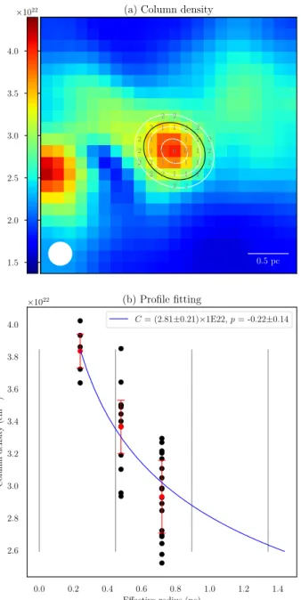
7. Column density and temperature structure
7.1. Calculation
In this section, we compare the differences between the struc-tures of different HMSCs. An isothermal, spherically symmetric prestellar clump with gravitational contraction is suggested have a clump radial density profile consisting of two regions: an inner core nH2=constant and envelope nH2 ∝ r−2(Vázquez-Semadeni
et al. 2019). The corresponding radial NH2 profiles are NH2 ∝ r
and NH2 ∝ r−1, respectively. Owing to the limited resolution, a
flat central region and truncated radius are usually set when fit-ting the NH2 profile to the observational data (Juvela et al. 2018;
Tang et al. 2018). The Galactic cold cores NH2 structures
inves-tigated with Herschel data indicate that radial NH2 distribution
follows a power law of NH2 ∝ r−1in spite of the broad variety
of clump morphology, which suggests the universality of the r−1
profile for cold cores with gravitational contraction (Juvela et al. 2018;Li 2018).
We compare NH2or Tdustradial profile of different HMSCs
with PPMAP data. Beam size is a crucial factor that could affect the clump structures we observed. A larger beam smooths the steep profile to make it flatter. Furthermore, beam size determines the lower size limit of the flat central region. The resolution of PPMAP Hi-GAL data, which is 1200, is more likely
to detect the envelope rather than the inner core of clumps at a distance of several kpc. We simply fit a single power law radial NH2profile NH2 =C × r
pNH2
to the PPMAP NH2 data rather than
with a more complex function.
Firstly, only AS and NA HMSCs with a mass larger than 100 M are considered to ensure the selection of massive
sources. The HMSCs with an angular size <2400 and distance
>8.34 kpc are removed to mitigate the resolution issue. Secondly, we separate the PPMAP pixels into a series of concentric ellip-tical shells with a shell width of 600 in minor axis, which is the
pixel size and the half beam size of PPMAP data. The aspect ratios and position angles of each elliptical shell of HMSCs are the same as the ellipses outlining the shapes of HMSCs in Y17. The radius of the largest shell is slightly larger than the clump size. For the pixels crossing the edges of the shells, we simply assign the associated shells according to the centers of these pixels. Thirdly, the median NH2 in one shell is used as the
NH2 in this shell whereas the 25th and 75th percentiles of the
pixel NH2of the shell are used as the error ranges of NH2for this
shell. Finally, the median NH2 in different shells are fitted with
a power-law profile NH2=C × r
pNH2
. An example of NH2 profile
fitting is shown in Fig.16. Similar operations are carried out on PPMAP Tdustimages to look at the temperature profile and get a
power-law index pTdust.
7.2. Properties and results
The NH2and Tdustpower-law indexes (pNH2 and pTdust) are shown
in Figs. 17a and b, respectively. The median value of pNH2 is
−0.17, which is much larger than the value of −0.85 inJuvela et al.(2018). There are several reasons for this difference. The clumps/cores they studied have a more compact morphology with a typical size of 0.075 pc compared to '0.5 pc for our HMSCs. Their beam size is equal to 0.03 pc with a typi-cal distance of 250 pc, but our beam size is 0.4 pc with a typical distance of 4 kpc. Our relatively poor physical resolu-tion could create a higher pNH2 value. Furthermore, their fitting
field is larger than the clump scale, which includes the weaker background emission that results in a smaller pNH2 value. Our


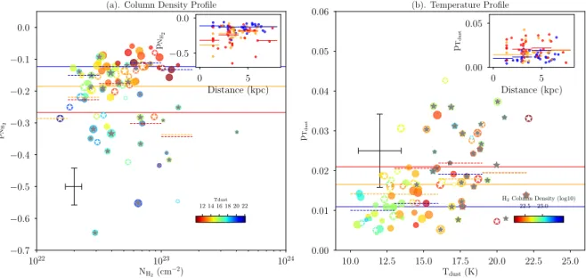
![[PDF] Formation jQuery pdf comment ca marche | Cours jquery](data:image/gif;base64,R0lGODlhAQABAIAAAP///wAAACH5BAEAAAAALAAAAAABAAEAAAICRAEAOw==)