HAL Id: hal-03026261
https://hal.archives-ouvertes.fr/hal-03026261v2
Preprint submitted on 8 Dec 2020
HAL is a multi-disciplinary open access
archive for the deposit and dissemination of
sci-entific research documents, whether they are
pub-lished or not. The documents may come from
teaching and research institutions in France or
abroad, or from public or private research centers.
L’archive ouverte pluridisciplinaire HAL, est
destinée au dépôt et à la diffusion de documents
scientifiques de niveau recherche, publiés ou non,
émanant des établissements d’enseignement et de
recherche français ou étrangers, des laboratoires
publics ou privés.
Size-independent phase distinction in dispersed
two-phase flows
David de Souza, Till Zürner, Romain Monchaux
To cite this version:
David de Souza, Till Zürner, Romain Monchaux. Size-independent phase distinction in dispersed
two-phase flows. 2020. �hal-03026261v2�
(will be inserted by the editor)
Size-independent phase distinction in dispersed two-phase
flows
David De Souza · Till Z¨urner · Romain Monchaux
Received: date / Accepted: date
Abstract Dispersed two phase flows cover a wide range of natural phenomenon and technological applications. When studying such complex systems, having access to the velocities of both phases is necessary to fully under-stand their dynamics. While data from both phases can be obtained in numerical simulations, this can prove more difficult to perform with experimental measure-ments. In this article, a new method to separate inertial particles from tracers in a two-dimensional laser sheet is described. By using a two camera acquisition system combined with an optical filter, the two phases can suc-cessfully be segregated, without relying on an apparent size or intensity difference between inertial particles and tracers. This allows for the velocities and positions of the particles to be measured in conjunction with the velocity field of the carrying phase. A series of tests are performed on the method. In addition to ensuring that the method functions in a satisfactory manner, these tests give guidelines on how to use the method correctly. To illustrate an application of this method, measurement results of ceramic particles settling in still water are presented.
Keywords Particle laden flow · PIV · PTV · Dyed tracers · Optical filtering
This work was supported by the French Direction G´en´erale de l’Armement (DGA) through the Agence de l’Innovation de D´efense (AID).
D. De Souza·T. Z¨urner·R. Monchaux
Institut des Sciences de la M´ecanique et Applications Indus-trielles (IMSIA),
ENSTA-Paris / CNRS / CEA / EDF / Institut Polytech-nique de Paris,
828 Boulevard des Mar´echaux, 91120 Palaiseau, France E-mail: [email protected]
1 Introduction
Particle laden flows are ubiquitous in natural and in-dustrial systems, and have received much attention in the last decades. When particle inertia is different from that of the fluid, the particle dynamic deviate from that of tracers which exactly follow fluid elements, and are usually used in fluid metrology to gain access to the fluid velocity field. Inertial particle trajectories sam-ple the flow non-uniformly (Maxey and Corrsin, 1980) leading to preferential concentration, some regions of the flow being more visited than others due to their local properties (high/low strain or vorticity, vanish-ing acceleration...). When the particle loadvanish-ing is high enough, preferential concentration can lead to the for-mation of denser regions where particles accumulate as originally found by Brown and Roshko (1974). This so called clustering can also be a consequence of the path history of particles and can thus occur in any region of the flow, regardless of its local properties (Gustavs-son and Mehlig, 2011). The high intermittency in the concentration field due to clustering and/or preferen-tial concentration can be an issue in many applications (e.g. for pollutant, plankton dispersion, mixing or fuel combustion in engines), but it may also have dramatic impacts on other relevant issues of particle laden flows: collisions, settling velocity alteration and carrier phase modulation. The collision probability depends on both the local particle concentration field and on the local velocity gradients (Falkovich et al., 2002). The settling velocity is altered as soon as the carrier flow is tur-bulent (Maxey and Corrsin, 1980) but also when the local particle concentration is dense enough (Aliseda et al., 2002; Monchaux and Dejoan, 2017; Huck et al., 2018). Both cases depend non-trivially on many physi-cal parameters (e.g. volume loading, phase density
ra-tios, turbulence level or particle size). How the back reaction by the particles on the continuous phase mod-ifies the carrier flow is just as complex and sensitive to the same parameters (Elghobashi and Truesdell, 1993; Eaton, 2009).
As direct on-site measurements of these processes (e.g. in clouds, marine snow, ash clouds or combustion chambers) are rarely possible, model experiments and numerical simulations are traditionally used to inves-tigate the very rich physics of these flows. Due to the complexity of solving the flow in the vicinity of large numbers of finite sized particles, this kind of direct ap-proach is still limited (Homann and Bec, 2010; Lucci et al., 2010). Usually, the Navier-Stokes equations are solved for the fluid and model equations are used for the particles. Unfortunately, the available analytical model equations for the dynamics of inertial particles are ob-tained under the limiting assumptions of point particles and very large density ratio (Maxey and Riley, 1983; Gatignol, 1983) and involve many terms that are most of the time neglected in numerical studies. In addition, to reduce the computation time required to explore the wide parameter space described above, most numerical studies do not consider the back reaction particles ex-ert on the fluid. Providing empirical models that allow for this back reaction to be numerically implemented without solving the whole velocity field in the neigh-bourhood of each particle is thus an essential challenge for the coming years.
To address this challenge, as well as providing model free data to understand the complex and intricate roles of the large number of parameters controlling particle laden flows, experiments have to provide detailed mea-surements in both phases, at the same time and loca-tion. Such measurements provide us with the slip veloc-ity between the two phases, fluid-particle correlations or at least fluid statistics at the particle positions. All these quantities are key ingredients to understand the mechanisms at work in preferential concentration, clus-tering, settling velocity and collision alteration, and car-rier phase modulation. Even though the development of such simultaneous measurements in both phases has started two decades ago (Towers et al., 1999), it is still far from being routinely used in laboratories and no commercial solution is available yet.
Fluid flow measurements are now available in any number of dimensions. Three dimensional (3D) Eule-rian velocity fields are accessible through particle im-age velocimetry (PIV), that can even be time-resolved under certain conditions. Using particle tracking ve-locimetry (PTV), Lagrangian particle trajectories can also be measured at sufficiently high time resolutions to allow acceleration statistics to be computed
(Ouel-lette et al., 2008). The main drawback of the 3D mea-surements is its usually very limited volume. Probing wider regions of flows from both PIV and PTV is still the private preserve of two dimensional (2D) systems. Pointwise (0D) systems are also often employed in mul-tiphase flow studies, particularly in wind tunnels to collect one dimensional (1D) data sets under Taylor hypothesis assumptions. These systems can be intru-sive (hot wires, optical probes) or not (laser Doppler anemometer, phase Doppler particle analysis), some of them being able to discriminate between phases, see for example Muste et al. (1998). However, it has been recently shown that the acquired 1D data may suffer from very strong biases that are difficult to overcome (Mora et al., 2018). In the following we will focus on 2D systems.
Most 2D systems can be equally used to perform measurements on fluid tracers or on inertial particles. Indeed, as they are usually designed to see and/or follow tracers that are smaller than inertial particles, it is thus quite simple to use these same systems to image and/or track inertial particles that are often more visible on the acquired images than the tracers. The difficulty in mea-suring both phases thus mainly relies on the simultane-ity, as these systems are usually not made to perform PIV on the fluid and PTV on the inertial particles at the same time. Several groups have designed such cou-pled measurement systems (see next two paragraphs) but, as mentioned above, it still remains a challenging issue. As both independent measurements are well de-veloped, the key issue for simultaneously probing both phase is to manage the segregation between tracers and inertial particles. Depending on the carrier fluid, usu-ally air or water, the tracer characteristics can be quite different. In water they are typically almost neutrally buoyant spherical particles whose diameters can range between 5 to 30µm. In air, 1 to 2 µm oil droplets are tra-ditionally used, but are increasingly replaced by 300µm inflated neutrally buoyant soap bubbles. Regarding in-ertial particles, the range of particle size used by the different authors varies on orders of magnitude accord-ing to the wide range of correspondaccord-ing applications. Larger particles are usually sand or beads whose di-ameters can be as large as a few millimetres while the smallest can be even smaller than tracers. While PIV tracers are designed to diffuse as much light as possi-ble, inertial particles in general cannot be tailored to this purpose and come as they are. Depending on their size and material, they may scatter very little light.
Most successes in simultaneous fluid/particle mea-surements have been obtained when a large scale sepa-ration exists between particles and tracers. In this case, a classical 2D PIV/PTV system is sufficient and
parti-cles and tracers are acquired on the same image by a single camera. Multiple authors designed different post-processing algorithms to achieve the segregation: sim-ple discrimination by spot size has been used since the early two phase measurements by Chen and Fan (1992) or Hassan et al. (1992), but more sophisticated algo-rithms taking into account, for example, the relative brightness of tracers and particles (Khalitov and Long-mire, 2002; Petersen et al., 2019), or filtering the tracers as a high frequency noise (Kiger and Pan, 2000) have been proposed. In many cases, the material and size differences between tracers and particles are obviously used in the separation algorithms.
In the absence of scale separation, a relevant idea is to use fluorescent dye. Under laser illumination, dyed tracers will emit light at a shifted wavelength while par-ticles will only diffuse the incoming light as is. This seems to provide an easy way to perform the segrega-tion. Single camera acquisitions can still be relevant if a colour camera is used. With green 532 nm laser and rhodamin coated tracers (a classical set-up), the green channel will ideally only see the particles while the red channel would only see the tracers. See Towers et al. (1999) for a more sophisticated application where both phases are dyed differently and a triple pulse laser is used to discriminate them. Unfortunately, the low reso-lution of colour cameras, the interpolation schemes used to compensate for the colour filtered array of pixels and the high level of induced pixel locking incite to avoid colour cameras. The obvious alternative is to use two cameras equipped with colour filters and aiming at the same field of view. The main issue then becomes the dif-ficulty in matching the acquired fields of view. This can be achieved by using beam splitters, or by positioning both cameras very close to each other, aiming at almost the same field of view, and using a stereoscopic PIV calibration procedure to match the fields of view (the latter being our proposition). The use of a beam splitter avoids sophisticated calibration procedures since both cameras actually aim at the same field of view, but it implies a somewhat complex mounting and more im-portantly the loss of half the light budget, which may be an issue when particles do not diffuse much light. This was nonetheless successfully implemented by El-himer et al. (2017). In their study, a “cross-talk” be-tween the two cameras remained. In fact, the inertial particles used were much larger than the tracers (more than 1 mm in diameter) and, due to their size, faint im-ages of the inertial particles could be seen on the tracer images, as the fluorescent light emitted by the tracers was also scattered by the particles. This was solved with an additional post processing to separate particles from tracers thanks to their difference in intensity. The
un-usual use of a stereoscopic PIV system is made more appropriate and accurate nowadays with the recent de-velopment of so-called self-calibration algorithms that allow to almost perfectly match both fields of views. For more details on this calibration procedure see Wieneke (2005). In any case (colour or greyscale cameras, beam splitters or not), experimentalists are left with two sets of images. On the “red” one, only dyed tracers are visi-ble, the flow field is thus easily accessible. However, on the “green” one, it might be more complicated. Indeed, the efficiency of the absorption and emission of the in-coming wavelength by the dyed tracers is not 100%. As a result, tracers also directly scatter a portion of the laser light and are thus visible on the “green” images alongside the particles. Poelma et al. (2007) also refer to this as “cross-talk” between images. In their study, they manage to get rid of this cross-talk because, due to scale and brightness separation, the tracers’ grey level is within background noise on the “green” images. When particles and tracers have similar sizes and when the particle material does not scatter much light, a way to remove tracers from these images has to be found.
In this article, we propose a method to achieve si-multaneous velocity measurements of particles and trac-ers when no scale or brightness separation is present, by masking the tracers on images with inertial parti-cles. The method developed here is generic and can be applied with most standard stereoscopic PIV systems. Section 2 of this article describes this method and out-lines its potential pitfalls. To ensure that the method works and to examine its limitations, various tests are performed on experimental data sets. These testing pro-cedures and their results are presented in section 3. Fi-nally, section 4 gives recommendations on the method application and showcases some results from real-life experiments before concluding in section 5.
2 Tracer masking method 2.1 Method description
An overview of the method can be found in figure 1. The method starts from two synchronised image sources: one camera recording both particles and tracers, and one camera that only sees tracers. In the following these are denoted as particle camera and tracer camera, re-spectively. Both cameras record greyscale images, giv-ing the light intensities IP(x, y) for the particle camera
and IT(x, y) for the tracer camera.
The fluid velocity field can be calculated directly from IT using PIV. To perform PTV on IP, inertial
Source
images
Particle Camera Tracer Camera
Particles and tracers Tracers only
Fluid velocity field Particle positions and velocities PIV Apply mask PTV Tracer mask
Fig. 1: Flowchart of the method for simultaneous parti-cle tracking and fluid velocity measurements by tracer masking. The illustration frames display particle and tracers with exaggerated color and size difference for easier distinction only.
achieved by creating a tracer mask from ITthat
effec-tively removes the tracers from IP. The inertial
parti-cles can then be tracked on the resulting filtered images. The characteristics on how to perform a good PIV or PTV will not be discussed in this article, and the pa-rameters involved in these techniques will only be men-tioned when relevant to the topic.
A flowchart of the mask creation process can be found in figure 2. The goal is to set the intensities of all pixels belonging to a tracer in IP to zero. The first
step is to detect the tracers on IT. This is done by
turn-ing ITinto a binary image BTthat sets all pixels that
belongs to a tracer in ITwith zero:
BT(x, y) =
(
1, IT(x, y) < thT
0, IT(x, y) ≥ thT
, (1)
where thTis the intensity threshold defining whether a
pixel belongs to a tracer or not. Using the colour code of figure 2, the area of interest here becomes a white background, while the black spots of the tracers are the regions that will be discarded. However, depending on the configuration of the image sources, small dis-crepancies in shape, intensity, or even positions of the
Thresholding thT Erosion by S Source tracer image IT Binarised image BT Final mask M
Fig. 2: Flowchart of the mask creation process. On BT
and M , areas in white represent pixel values of one and areas in black are pixel values of zero.
tracers might exist between IP and IT. These are
fur-ther discussed in section 2.2. To accommodate for these discrepancies, the second step of the mask creation pro-cess increases the area of the tracers in BT. This is
done by performing an erosion of the white background around the black tracer spots using a structuring ele-ment S. This erosion is a morphological operation that will widen every area of BT where pixels are at zero,
i.e., marked as a tracer position. Examples of structur-ing elements can be found in figure 3. The larger S is, the more the black area will widen. For example, S1
does not change BT, S5sets to zero all pixels vertically
or horizontally adjacent to a zero, S9 adds all pixels
diagonally adjacent, etc. More details on such morpho-logical operations can be found in Haralick et al. (1987). The result of the erosion of BT by S is the final tracer
mask M .
The tracers are then removed from IP. This removal
is done by applying M to IP with a simple pixel-wise
multiplication:
IM(x, y) = IP(x, y)M (x, y), (2)
where IM is the final particle image, without tracers.
The positions and velocities of the inertial particles can finally be obtained by performing PTV on IM.
2.2 Error assessment
Generally speaking, errors resulting from the applica-tion of this method can have two main origins. The
Fig. 3: Examples of structural elements, which are usu-ally small binary sets. Each sub-square represents a pixel, zeros are in black, ones are in white. For the pur-pose of this article, they are designated by the number of pixels having a value of one. Essentially, for an ero-sion, any pixel that is at zero will result in all neighbour-ing pixels to be turned to zero to match the shape of S. For a given reference pixel at zero: S1 does not change
the image, S5turns all pixels vertically and horizontally
adjacent to the reference pixel to zero, S9does the same
but also sets pixels diagonally adjacent to zero, and so on. The structural elements represented here are also the ones used in the testing procedures of section 3.
discrepancies in the tracers properties between the two source images IPand ITconstitute one of these origins.
For example, if a system with two cameras is used, a tracer can be projected onto each camera with different intensities, shapes and positions. A difference in inten-sity is not an issue for the method presented here, as the choice of thTis informed by the intensities of tracers in
ITonly, and tracers masked in ITwill be removed from
IP regardless of their intensities. However, differences
in shape or position may lead to M not properly cover-ing the tracers in IP. In this instance, tracers detected
in ITmay remain in IM and particles might have been
erroneously deleted by the mask. The second category of error sources is an inadequate choice of the method parameters thT and S. Going to extreme cases, if thT
is low enough to catch the background noise level of IT, pixels that are not from tracers will be set to zero
in BT, resulting in an unnecessary loss of data in IM.
Conversely, putting thT too high will leave all tracers
in the image. For S, if it is too small, the erosion will not make up for the discrepancies between IP and IT.
But picking one that is too big will end up with a mask that deletes portions of the image that could have been kept.
From these two origins, three main errors can oc-cur: tracers can remain in IM, particles can be
com-pletely removed when applying the mask or they can be partially removed. These errors will be referred to as false particle error, erased particle error and altered particle error respectively. First, the false particle er-ror adds false positives, which can skew the tracking results as tracers are mistaken as particles. Second, the erased particle error leads to false negatives, resulting
(a) (b) Particle camera Laser sheet Main tank Injection column Seeding system Tracer camera
Fig. 4: Experimental set-up: (a) overview without the cameras, (b) top view.
in a loss of data. Finally, the altered particle error will change the particle’s detected position, as altering the shape of a particle will change where the center of the particle is detected. In addition to their effects on the trajectories computed by PTV, these errors will influ-ence the apparent concentration field, which is crucial to understanding the mechanics of dispersed two-phase flow systems.
3 Method Validation
To evaluate the response of the method to the errors outlined in section 2.2, two testing procedures have been devised. These procedures involve images from ex-periments as the basis of the tests. This section first describes the experimental set-up used to obtain these images before covering each testing procedure and their results.
3.1 Experimental set-up
An illustration of the experimental set-up can be found in figure 4. The main part is a tank of dimension 350 × 480 × 350 mm3. A column, of square cross-section with
side length 130 mm and height 410 mm, sits on top of it. This structure is filled with water. On top of the col-umn, a vibrating sieve serves as the seeding system for the apparatus. Particle injection is controlled by pour-ing particles onto the sieve and turnpour-ing the vibration on.
Observations are done in the main tank. Images are recorded with a LaVision stereo PIV acquisition sys-tem of two VC-Imager SX 4M cameras synchronised with a vertical pulsed laser sheet of wavelength 532 nm produced by an Nd:YAG Dual Power 135-15 laser from
Dantec Dynamics. The tracers used are coated in rho-damine. Accordingly, the tracer camera is equipped with an optical filter that lets the fluoresced light emitted by the rhodamine of wavelength above 570 nm pass through and blocks the laser wavelength. Both cameras are calibrated on the same area of the laser sheet using a dotted plate and the self-calibration method previously mentioned.
The two cameras record two images or frames each, in quick succession, and the time in between the two frames can range from 10 to 30000 µs. These double frames from both cameras are recorded with an acquisi-tion frequency of up to 15 Hz. After applying the tracer removal method, the instantaneous particle positions and velocities, and the fluid velocity field are obtained. However, the maximal sampling frequency of the sys-tem does not allow to track particles between double frames, i.e., long-term particle trajectories are not ac-cessible in the present experiments. In other terms, PTV is performed on each double frame recorded as if it were independent of the previous and following double frames in the experiment. However, the method pre-sented in this article does not depend on the acquisi-tion frequency and and can be applied to systems with higher sampling rates.
The images have a resolution of 1700 by 2375 pixels, with each pixel having an intensity ranging from 0 to 4095. Overall the acquisition system has a scaling factor of 13.7 pixel/mm which then corresponds to an area of 124 by 173 mm of the laser sheet used for observation. For each experiment, an image of the minimal intensi-ties observed on the experimental run is computed and then subtracted from all images to increase the signal to noise ratio. After this operation, the images typically have a background noise below 10 in pixel intensity. The apparent diameter in pixels of the particles obvi-ously depend on their size and the material they are made of but the smallest tested up to now span 4 to 5 pixels. The rhodamine coated tracers have an apparent diameter of 2 to 3 pixels.
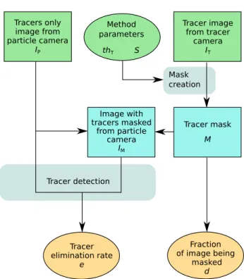
3.2 Tracer removal test procedure
The first testing procedure is a tracer elimination check done mainly to test the method’s response to the er-rors from the discrepancies between IP and IT, and
how its parameters can be tuned to yield reliable re-sults. A flowchart of this procedure can be found in figure 5. It is designed to ensure that the method re-moves all tracers while deleting as little of the image as possible. The test images IP and ITused here contain
only tracers. That way when applying the tracer mask-ing method, the resultmask-ing IM should ideally be empty.
Tracers only image from particle camera IP Tracer image from tracer camera IT Tracer mask M Image with tracers masked from particle camera IM Tracer detection Tracer elimination rate e Fraction of image being masked d Mask creation thT S Method parameters
Fig. 5: Flowchart of the testing procedure on errors coming from discrepancies between IPand IT.
Then, by applying PTV on IM, any particle detected
will in fact be a tracer that was not removed. The im-ages IPand ITused were taken from experiments
con-ducted on the device described in section 3.1. For a given pair of tracer-only images IP and IT, the only
other inputs for the testing procedure are thT and S,
the parameters of the tracer removal method. A parti-cle detection (i.e., the first step of PTV) is performed on the tracer-only particle image IPand on the masked
image IM, resulting in a number of detected particles
for each of these images. These numbers will respec-tively be called NP and NM. A tracer elimination rate
e is then computed as e = (NP− NM)/NP. In addition,
the fraction d of the image deleted by the method can also be computed from the mask itself, as the number of pixels at zero in the mask over the total number of pixels. An overview of the inputs used for this testing procedure can be found in table 1.
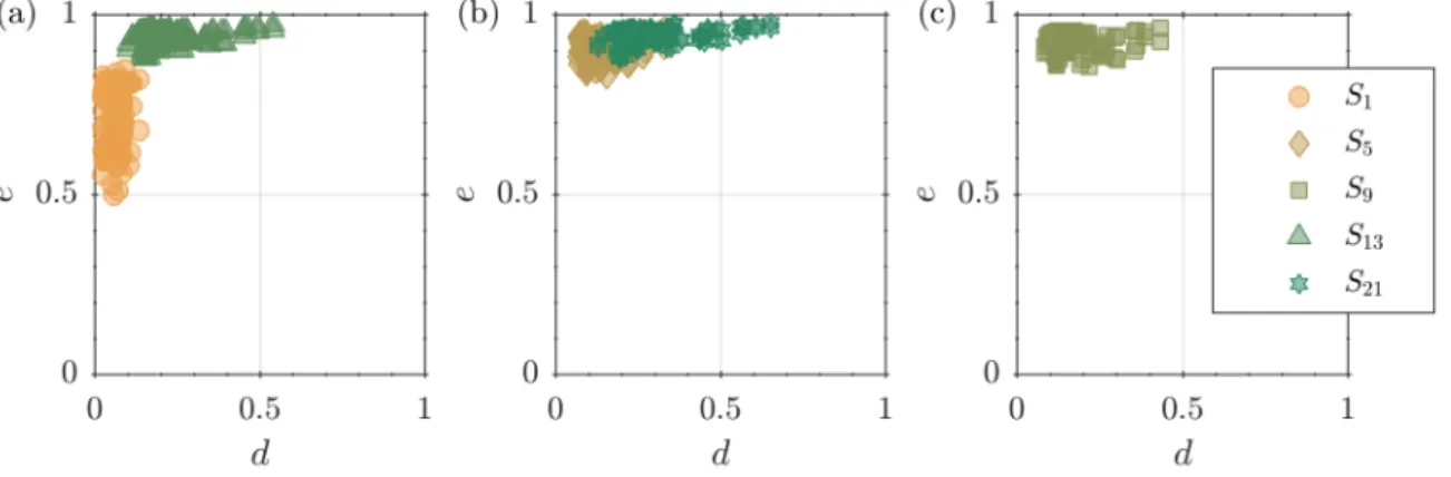
Both e and d take values between zero and one. Ide-ally, e should be as close to one as possible and d should remain close to zero. In figure 6, e is plotted against d, separated and coloured by values of thTused in the
tests. thTis shown to have a clear impact on both e and
d. The observed response can be explained as follows. Taking a value for thTthat is too low will identify the
Table 1: Overview of the parameters tested in the tracer removal test procedure (section 3.2), and of the charac-teristics of the images tested. For an illustration of the structuring elements’ shapes, see figure 3. All the images used are from different experimental runs. The tracer brightness given is for well lit tracers in the laser sheet, i.e. tracers that are fully in the laser sheet.
Parameter Values, range or number Unit
thT {5; 10; 20; 35; 50; 70} greyscale intensity Structuring elements’ shapes S1,S5,S9,S13,S21
-Number of images 77
-Tracer diameter 2 to 3 pixel
Fig. 6: Scatter plots of e against d, distinguished by values of thT, for all S. These are spread in three separate
plots for clarity, to avoid overlapping too many points. Among the tested thresholds, thT= 20 (squares) results
most consistently in low d and high e.
Fig. 7: Scatter plots of e against d, for thT = 20 (square markers in figure 6(c)), distinguished by S. These are
spread in three separate plots for clarity, to avoid overlapping too many points. S5 and S9lead to the best results
area removed by the mask to regions where there are in fact no tracers. This results in all tracers being removed but at the cost of deleting a large portion of the image, thus in high e and high d. On the other hand, setting a value for thT that is too high will miss a lot of the
tracers in IT, causing them to remain after M has been
applied, as described in section 2.2. As fewer tracers are marked for removal, a smaller fraction of the image will be deleted, which leads to both low e and low d. thT
needs to be selected carefully in order to get appropri-ate results, i.e., high e and low d. In the tests presented here, thT = 20 (squares in figure 6) seems to achieves
the best results in terms of high tracer elimination e and low image deletion d. Note that this value is specific to the images tested here, and depends on the image ac-quisition system and potential post-processing applied to the image (such as background image subtraction or noise filtering). The method may still perform well for thT< 20, as, even if more of the image is deleted, more
tracers will be removed without necessarily diminishing the number of inertial particles that can still be found by the method.
The impact of S can then be seen in figure 7, where e is plotted against d for a fixed thT = 20, separated
and coloured by S. S1, which in facts corresponds to
no erosion being performed at all, does not remove all tracers but keeps d at low values. By increasing the size of the structuring element to S5 and S9, e gets higher
without deleting too much of the image yet. Beyond that for S13 and S21, e remains in the same range but
d increases. Overall, this is because larger S widen the areas detected as tracers more than smaller S when ap-plying the erosion. This results in smaller S deleting less of IPthan larger ones but also being less likely to catch
discrepancies between the position or shape of a tracer in IT and in IP. The images IP and IT used in these
tests match one another with a precision of ±1 pixel. This explains the better results obtained for S5 and S9
as these two elements extend the areas detected as trac-ers in BT over that ±1 pixel range for the final mask
M .
This procedure confirms the trends mentioned in section 2.2 on the influence of the choice of thT and
S. These parameters need to be chosen carefully and tuned according to the images and the system used.
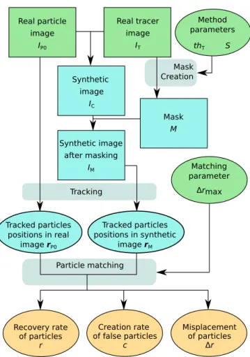
3.3 Particle matching test procedure
The second procedure is designed to test errors result-ing specifically from an inadequate choice of the pa-rameters thTand S. A flowchart of this procedure can
be found in figure 8. The objective here is to ensure that tracked particles can faithfully be recovered after
Real particle image IP0 Real tracer image IT Synthetic image IC Mask M Synthetic image after masking IM Tracked particles positions in real image rP0 Tracked particles positions in synthetic image rM Tracking Particle matching Recovery rate of particles r Creation rate of false particles c Misplacement of particles Δr Mask Creation thT S Method parameters Matching parameter Δrmax
Fig. 8: Flowchart of the testing procedure on inadequate parameter choice.
the method has been applied, while still removing the tracers. To separate this test from errors coming from discrepancies between IP and IT, it is performed on
images with a perfect superposition between the two cameras. To achieve this, an image where only parti-cles are visible IP0 is taken and combined with a tracer
image IT into a synthetic image IC. IC is made by
taking the maximal intensity between IP0 and IT for
each pixel: IC(x, y) = max(IP0(x, y), IT(x, y)). By
do-ing so, IC has both particles and tracers, tracers
per-fectly match between ITand IC, and IP0gives access to
what IClooks like without tracers. The goal is then to
recreate IP0 by applying the tracer removal method to
IC and see if tracking results are the same when PTV
is performed on IP0 and on IC after removing the
ar-tificially added tracers. The tracer removal method is used on IC which results in a masked image IM, and
PTV is then performed on IP0 and IM. This gives
ac-cess to the positions rP0 and rM of particles
track has been found, providing both particle position and velocity). A particle matching is then performed, by comparing the particle positions rP0 and rM,
pair-ing particles in IP0 and IC with a maximal distance
between them of ∆rmax. Overall, the inputs of this
test-ing procedure for a given pair of images IP0and ITare
the method parameters thT and S, and the matching
parameter ∆rmax. After the particle matching is done,
particles can be divided into three categories: particles only found in IP0, particles only found in IM, and
par-ticles that have been successfully matched between IP0
and IM. The number of particles in each of these
cat-egories are denoted as NP0, NM and Nb, respectively.
The rate of particle recovery r is then computed as: r = Nb/(Nb+ NP0). r then varies between zero and
one, with zero meaning that all initially tracked parti-cles in IP0 were lost while going through the test, and
one meaning that all of them where recovered. In the same manner, the tracers left in IM appear as newly
created particles, and correspond to the number NM.
Accordingly, the creation of false particles is computed by the creation rate c, given by: c = NM/(Nb+ NP0).
Additionally, the particle matching gives the misplace-ment ∆r for each particle detected in both IP0 and IM,
that is to say ∆r = ||rM− rP0||.
An overview of the input parameters used in this procedure is presented in table 2. Although tests have been performed for all the structuring elements S pre-sented in figure 3, the best results where systematically obtained with S1, which is equivalent to not applying
any erosion when making the mask. This is in line with the fact that, in this testing procedure, the images have a perfect superimposition, and the areas of the mask that will remove the tracers do not need to be extended to cover any discrepancies between the particle image and the tracer image. All data presented in this sec-tion hereafter is obtained using S1 as the structuring
element.
As ∆rmax fixes the maximum misplacement error
that can be measured in these tests, its value may influ-ence the results obtained by the procedure. To avoid the introduction of biases, the mean recovery and creation rates hri and hci (averaged over all test cases for a given thT) are plotted against ∆rmax in figure 9. For ∆rmax
between 1 and 2 pixel, hri and hci saturate on plateaus whose values depend mainly on the chosen threshold thT. This fixes an upper limit to the misplacement of
particles by the method to 2 pixels, as increasing ∆rmax
beyond this value does not change the results. This limit can be high depending on the resolution of the system, but will be discussed further at a later point in this sec-tion. To further study r and c, ∆rmax = 2 pixels will
be used in the following analysis.
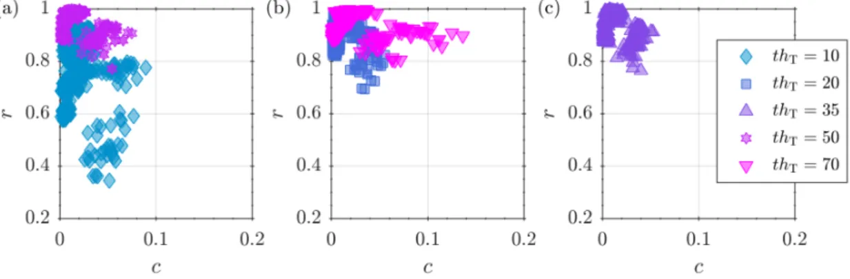
For this procedure, a good parameter choice should result in high r and low c. Here, again, thT is shown
to be crucial. Scatter plots of r against c distinguished by thT are represented in figure 10. Over these plots,
as thT increases, r increases overall to values getting
closer to one. The values of c start spread over a 0 to 0.1 range for thT = 10. That range first decreases as
thTincreases, reaching a minimal spread for thT= 35.
For thT values above that, the range of c values
in-creases again. This confirms yet again that picking too low or too high of a value for thT leads to poorer
per-formance for the method, as low values generate masks that cover a larger area than necessary and high values fail to remove some tracers. Over the tests presented here, thT= 35 seems to achieves the best results.
By design of the test method, for each set of given inputs, ∆r ≤ ∆rmax. To obtain a finer measure of the
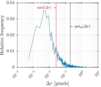
misplacement error of the method, the distribution of ∆r has to be studied. The misplacements ∆r of all de-tected particles have been compiled in histograms such as the one presented in figure 11. All histograms ob-tained are heavily skewed toward low values for ∆r, typically less than 0.1 pixel. To have a better estimation of the misplacement error, the median and 90th
per-centile of the distribution of ∆r have been computed for every test case. Figure 12 shows these quantities av-eraged for a given thTand ∆rmax. Both the median and
90th percentile of ∆r have a minimal value reached for
thT = 35 in the tested cases, confirming the previous
result that this is the best value for thTover the tests
made in this procedure. In this case, half of the par-ticles are on average misplaced by less than 0.05 pixel by the method, and 90% by no more than 0.21 pixel. These results are also stable for ∆rmax> 2 pixel, while
values lower than that lead to slightly lower values of the median and 90th percentile.
4 Method results 4.1 Recommendations
The starting step to use the method is to acquire the im-ages. First, the tracer images should be suitable to per-form PIV. This means having a sufficient tracer seeding in regard to the image resolution and the PIV interro-gation windows, typically 3 to 5 tracer per interroga-tion window. However, as the method removes the part of the image that corresponds to tracers, it is recom-mended to aim at the lowest possible density in trac-ers that still allows PIV to be performed. This will of course be dependent on the acquisition system and on the PIV algorithm used. Secondly, the particle images should also enable PTV to be performed. Overall, this
Table 2: Overview of the parameters tested in the particle matching test procedure. For an illustration of the structuring elements’ shapes, see figure 3. The images ITand IP0 come from various experiments using tungsten
carbide particles of diameter comprised between 63µm and 75 µm and ceramic particles with diameters between 180 µm and 200 µm.
Parameter Values, range or number Unit
thT {10; 20; 35; 50; 70} greyscale intensity
∆rmax 0.2 to 5 pixel
Structuring elements’ shapes S1,S5,S9,S13,S21
-Number ofIT 6
-Number ofIP0 75
-Tracer diameter 2 to 3 pixel
Particle diameter 4 to 7 pixel
Fig. 9: Averages of r and c, as functions of ∆rmax, coloured and separated by thT. Only some values of thT are
presented here to show the general trends. The error bars are of one standard deviation above and below the mean value. Both hri and hci stabilise at plateau values reached generally between 1 to 2 pixels for ∆rmax. These plateau
values are mainly influenced by thT.
Fig. 10: Scatter plots of r against c for ∆rmax= 2 pixel, distinguished by values of thT. These are spread in three
separate plots for clarity, to avoid overlapping too many points. The threshold that reaches high r and low c most consistently is thT= 35.
Fig. 11: Typical example of an histogram of ∆r. The counts are normalised by the total number of samples (i.e., the number of particles successfully matched Nb)
to obtain a relative frequency. This histogram comes from a test case with thT= 35, S1and ∆rmax= 2
pix-els. The median and 90th percentile of the distribution are marked by vertical lines.
also translates to having a good resolution of the par-ticles on the images to accurately find particle posi-tions. Once again this will depend on the systems and algorithms used. For the acquisition system presented in section 3.1, having an apparent diameter of 5 pix-els was enough to detect particle centers with sub-pixel precision. Finally, and perhaps most importantly, both image sources must be synchronised and calibrated in a way that allows them to be superimposed. The su-perposition should be as accurate as possible, to allow for a smaller structuring element S to be used which reduces the risk of erroneously deleting particles with the tracer mask (see section 3.2).
To use the method itself, the choice of thT is the
most important parameter to decide on, as evidenced by the tests of sections 3.2 and 3.3. thTshould be
cho-sen so that it is above the background noise of IT, to
avoid the removal of portions of the image where no tracers are present. Other than that, we recommend to set thT as low as possible to ensure all tracers are
removed. Typically, for the images obtained from the experimental set-up described in section 3.1, thT= 10,
when paired with S9results in almost all tracers being
eliminated from IPwhile still being able to track at the
very least 80% of inertial particles.
The choice of the structuring element S is then also important. This will depend on how well IP and IT
can be superimposed. In the case of a perfect
superpo-Fig. 12: Mean of the median and 90th percentile of ∆r over the tested cases against thT, and separated by
∆rmax. Three ∆rmax have been chosen here to
show-case the trends observed. The results for ∆rmax = 2
(in red) and ∆rmax= 4 (in green) are almost
superim-posed.
sition, (i.e., all tracers in both images perfectly over-lap) no erosion (S1) is required for the method to work
correctly. Otherwise, a measure of how much dispar-ity remains between IP and IT is needed to choose the
structuring element. A simple approach is to perform a cross-correlation on sub-areas of images IP and IT
when only tracers are visible. This is in fact similar to how the correction from the self-calibration method is computed (Wieneke, 2005), and akin to how PIV is performed in general. The resulting disparity map gives the remaining local misplacement between IP and IT.
Then the larger the disparities are, the larger S will have to be. For example, for differences of ±1 pixels, S9 would be a good choice, as this element will cover
all disparities in that range.
Finally, we would like to point that the structur-ing elements tested here where chosen to have no pref-erential orientation. This is because the present dis-crepancies between IP and IT did not show any
set-up, anisotropic distortions can occur and remain consistent through time. Examples of such distortions include curved windows between the cameras and the laser sheet (e.g. cylindrical tanks) or astigmatism which can be induced by some optical filters. When such time-consistent distortions occur, S can also be deformed and stretched along the direction of these distortions.
4.2 Example results
This section showcases some results obtained with the tracer removal method. Those results come from an ex-periment where ceramic particles with diameters be-tween 160 nm and 180 nm are settling in water. The fluid is initially quiescent and seeded with tracers coated in rhodamine. The experiment is performed in the ex-perimental set-up described in section 3.1. The record-ing starts as soon as the seedrecord-ing system is turned on (t = 0 s).
Figure 13 shows the evolution of the vertical veloc-ity vz of the detected particles over time. Histograms
of vz have been computed for each timestep and
com-piled into a colour plot. Additionally, the mode of the histogram is shown as a solid line. Negative values of vz denote a downward motion of the particles. In the
first instants, the particles have not reached the field of view of the cameras so any detected particles are false positives from tracers, which explains the histograms’ modes lingering around vz ≈ 0. At t = 12 s particles
start passing in the camera field of view and can be de-tected. The first cloud of particles falls with a settling speed of vz≈ −0.32 m/s. In their wake, subsequent
par-ticles are accelerated to velocities of vz ≈ −0.42 m/s
(t ≈ 40 s). Finally, the particles reach a stationary behaviour (t > 90 s) while falling with a velocity of vz≈ −0.34 m/s.
Figure 14 shows two examples of instantaneous par-ticle velocities and fluid vertical velocity fields from the same experiment. They were taken at t = 20 s for fig-ure 14a and t = 60 s for figfig-ure 14b to have similar average particle velocities. Figure 14a shows the parti-cles settling in a column with a downward fluid flow. The same can be said for figure 14b, however the num-ber of particles is smaller and the downward fluid flow is more intense and localised in the column of settling particles. The evolution of the fluid velocity flow suggest the development of large scale flows in the experimental set-up.
The tracer removal method could then give access to data from both phases simultaneously and showcase the importance of having access to both velocity fields to better study dispersed two-phase flow systems. Statis-tics on the evolution of other relevant quantities such
as the local slip velocity (i.e., the difference between the particle velocity and the fluid velocity at the position of the particle) will be investigated in future studies.
5 Conclusion
A method to distinguish particles from tracers in the study of dispersed two-phase flow has been developed. This method relies on the use of both optical filtering paired with adequately dyed tracers (rhodamin coated tracers in this case) and post-processing operations to segregate inertial particles from tracers. This tracer re-moval method can function properly even when parti-cles and tracers are undistinguishable in size or inten-sity through usual visualisation techniques. The method was tested to ensure its proper operation, and to assess its response to various input parameters. From these tests, suitable parameters for the method were found. Although these parameters are specific to the exper-imental set-up on which the method is used, general rules on how to properly choose them have been pro-vided. This method works on a variety of particle ma-terial and size, opening the possibility to access large ranges of the parameter space experimentally.
Conflict of interest
The authors declare that they have no conflict of inter-est.
Appendix: Exemplary implementation
This section outlines an example implementation of the tracer removal method in MATLAB R2016b. The particle imageIP and the tracer imageITare stored in the variablesI PandI T, respectively, as (N1× N2)-matrices of typeuint16. The posi-tion of the tracers inITare detected by a threshold valuethT of, for example, 35.
>> th T = 35; >> B T = I T < th T;
The variable B Tholds the binarised image BT. For the erosion ofBT, the structure elementS5is chosen.
>> S 5 = [0 1 0; 1 1 1; 0 1 0]; >> M = imerode(B T, S 5);
The variableMis a (N1× N2)-matrix of typelogical con-taining the tracer maskM. To calculate the masked particle imageIM, the mask is applied toIP.
>> I M = I P .* cast(M, ’like’, I P);
The variableI Mis a (N1× N2)-matrix of typeuint16and contains the imageIMwith only particles remaining. It can now be further evaluated, for example, by applying a PTV algorithm.
Fig. 13: Temporal histogram the vertical velocity vzfor ceramic particles of diameters between 160 nm and 180 nm
settling in quiescent water. The black line corresponds to the mode of the histogram at each instant in time. The vertical axis z of the experiment is oriented upward, so falling particles have negative velocities.
(a) (b)
Fig. 14: Instantaneous particle velocities (arrows) and fluid vertical velocity fields uz (color-plot) at (a) t = 20 s
and (b) t = 60 s, of the same experiment shown in figure 13. Arrows of the average velocity magnitude of the particles are in the top-left corners of each plot for scale.
References
Aliseda A, Cartellier A, Hainaux F, Lasheras JC (2002) Ef-fect of preferential concentration on the settling velocity of heavy particles in homogeneous isotropic turbulence. Jour-nal of Fluid Mechanics 468:77–105
Brown GL, Roshko A (1974) On density effects and large structure in turbulent mixing layers. Journal of Fluid Me-chanics 64:775–816
Chen R, Fan LS (1992) Particle image velocimetry for charac-terizing the flow structure in three-dimensional gas-liquid-solid fluidized beds. Chemical Engineering Science 47(13-14):3615–3622
Eaton JK (2009) Two-way coupled turbulence simulations of gas-particle flows using point-particle tracking. Interna-tional Journal of Multiphase Flow 35(9):792–800
Elghobashi S, Truesdell G (1993) On the two-way interac-tion between homogeneous turbulence and dispersed solid particles. I: Turbulence modification. Physics of Fluids A: Fluid Dynamics 5:1790
Elhimer M, Praud O, Marchal M, Cazin S, Bazile R (2017) Simultaneous PIV/PTV velocimetry technique in a turbu-lent particle-laden flow. Journal of Visualization 20(2):289– 304
Falkovich G, Fouxon A, Stepanov MG (2002) Acceleration of rain initiation by cloud turbulence. Nature 419:151–154 Gatignol R (1983) The Faxen formulae for a rigid
parti-cle in an unsteady non-uniform Stokes flow. Journal de M´ecanique Th´eorique et Appliqu´ee 2:143–160
Gustavsson K, Mehlig B (2011) Ergodic and non-ergodic clus-tering of inertial particles. Europhysics Letters 96(6):60012 Haralick RM, Sternberg SR, Zhuang X (1987) Image Analysis Using Mathematical Morphology. IEEE Transactions on Pattern Analysis and Machine Intelligence PAMI-9(4):532– 550
Hassan Y, Blanchat T, Seeley Jr C, Canaan R (1992) Simul-taneous velocity measurements of both components of a two-phase flow using particle image velocimetry. Interna-tional Journal of Multiphase Flow 18(3):371–395
Homann H, Bec J (2010) Finite-size effects in the dynamics of neutrally buoyant particles in turbulent flow. Journal of Fluid Mechanics 651:81–91, 0909.5628
Huck P, Bateson C, Volk R, Cartellier A, Bourgoin M, Aliseda A (2018) The role of collective effects on settling velocity enhancement for inertial particles in turbulence. Journal of Fluid Mechanics 846:1059–1075
Khalitov D, Longmire E (2002) Simultaneous two-phase piv by two-parameter phase discrimination. Experiments in Fluids 32(2):252–268
Kiger K, Pan C (2000) PIV technique for the simultaneous measurement of dilute two-phase flows. Journal of Fluids Engineering 122(4):811–818
Lucci F, Ferrante A, Elghobashi S (2010) Modulation of isotropic turbulence by particles of Taylor length-scale size. Journal of Fluid Mechanics 650:5
Maxey M, Corrsin S (1980) Stokes spheres falling under grav-ity in cellular flow-fields. APS Bulletin 25:paper EA6 Maxey MR, Riley JJ (1983) Equation of motion for a small
rigid sphere in a nonuniform flow. Physics of Fluids 26:883– 889
Monchaux R, Dejoan A (2017) Settling velocity and prefer-ential concentration of heavy particles under two-way cou-pling effects in homogeneous turbulence. Physical Review Fluids 2(10):104302
Mora DO, Aliseda A, Cartellier A, Obligado M (2018) Pitfalls measuring 1d inertial particle clustering. In: iTi Conference
on Turbulence, Springer, pp 221–226
Muste M, Fujita I, Kruger A (1998) Experimental comparison of two laser-based velocimeters for flows with alluvial sand. Experiments in Fluids 24(4):273–284
Ouellette NT, OMalley P, Gollub JP (2008) Transport of finite-sized particles in chaotic flow. Physical Review Let-ters 101(17):174504
Petersen AJ, Baker L, Coletti F (2019) Experimental study of inertial particles clustering and settling in homogeneous turbulence. Journal of Fluid Mechanics 864:925–970 Poelma C, Westerweel J, Ooms G (2007) Particle fluid
in-teractions in grid-generated turbulence. Journal of Fluid Mechanics 589:315–351
Towers D, Towers C, Buckberry C, Reeves M (1999) A colour PIV system employing fluorescent particles for two-phase flow measurements. Measurement Science and Technology 10(9):824
Wieneke B (2005) Stereo-PIV using self-calibration on parti-cle images. Experiments in Fluids 39(2):267–280