HAL Id: hal-01876406
https://hal.archives-ouvertes.fr/hal-01876406
Submitted on 20 Sep 2018
HAL is a multi-disciplinary open access
archive for the deposit and dissemination of
sci-entific research documents, whether they are
pub-lished or not. The documents may come from
teaching and research institutions in France or
abroad, or from public or private research centers.
L’archive ouverte pluridisciplinaire HAL, est
destinée au dépôt et à la diffusion de documents
scientifiques de niveau recherche, publiés ou non,
émanant des établissements d’enseignement et de
recherche français ou étrangers, des laboratoires
publics ou privés.
Adaptive Exponent Parameter: a Robust Control
Solution Balancing Between Linear and Twisting
Controllers
Elias Tahoumi, Franck Plestan, Malek Ghanes, Jean-Pierre Barbot
To cite this version:
Elias Tahoumi, Franck Plestan, Malek Ghanes, Jean-Pierre Barbot. Adaptive Exponent Parameter:
a Robust Control Solution Balancing Between Linear and Twisting Controllers. Variable Structure
Systems, 2018, Graz, Austria. �hal-01876406�
Adaptive Exponent Parameter: a Robust Control Solution Balancing
Between Linear and Twisting Controllers
Elias Tahoumi, Franck Plestan, Malek Ghanes and Jean-Pierre Barbot
Abstract— In this paper, a new controller is proposed, based on a well known homogeneous controller. The suggested con-troller gives rise to an efficient trade-off between the standard linear state feedback and twisting algorithm. As a consequence, the obtained controller has the advantages of both controllers with their drawbacks reduced. To achieve this objective, a parameter on the exponent terms of the homogeneous controller is adapted. The convergence of the closed loop system to a vicinity of the origin is given. Finally, some simulations validate the effectiveness of the proposed controller.
I. INTRODUCTION
It is in general a delicate task to mathematically model the dynamics of physical systems as well as the perturbations that are acting on them. These systems belong to the family of uncertain systems for which many control laws do not result in the desired behavior.
Sliding mode control [14], [17] is a well known technique designed to control such systems mainly because of its robust property. Among sliding mode controllers, one can cite standard (first order) ones that give rise to the chattering phenomenon due to the “sign” function used in the control. These high frequency oscillations can damage actuators. In order to reduce the effect of this phenomenon, higher order sliding mode algorithms [1], [5], [6], [8], [9] have been proposed. The concept is to use the higher order time derivatives of the sliding variable in the control. However, the use of higher order time derivatives engenders noise. Moreover, standard and higher order sliding modes are high energy consuming (from a control effort point of view) since only the bounds of the uncertainties and perturbations are considered known and therefore the gains are usually overestimated. A method that reduces the chattering effect as well as the energy consumption is the adaptive gain sliding mode technique [3], [11], [15], [16]. The idea is to dynamically adapt the controller gains depending on sliding mode establishment. However, accuracy can be affected due to the loss of sliding mode, because the controller gain transitorily becomes too small with respect to uncertainties and perturbations.
The problem under interest is the control of an uncer-tained/perturbed system of relative degree equal to two with respect to the sliding variable. Several methods have been designed to stabilize this kind of systems, notably the twistingalgorithm, which is known for its high precision and E. Tahoumi, F. Plestan and M. Ghanes are with Ecole Centrale de Nantes, LS2N UMR CNRS 6004, 44321 Nantes , France (e-mail: [email protected]; [email protected]@ec-nantes.fr; [email protected])
J-P. Barbot is with ENSEA, Quartz EA 7393, 95014 Cergy-Pontoise, France (e-mail: [email protected])
robustness. However, since the controller is discontinuous, the reduction of the chattering effect is limited and the controller is relatively high energy consuming.
Another control solution is using a linear state feedback. This latter is smooth and low energy consuming. In fact, in the absence of uncertainties/perturbations, the error and energy consumption tend towards zero in the steady state. However, the closed loop system is highly sensible to un-certainties/perturbations where the accuracy becomes low in their presence.
In this work, a new scheme of control is proposed with the advantages of both the twisting control (robustness and accuracy) and the linear state feedback (low energy consumption). Inspired by [2], the proposed scheme allows to achieve an efficient trade-off between the linear state feedback and twisting algorithm by varying the parameter on the exponent terms of the controller [2]. It is well known that the controller proposed in [2] is homogeneous [10], [13]. To the best knowledge of the authors, there is no result yet in the literature dealing with a variable parameter on the exponent terms of homogeneous controller schemes. The paper is organized as follows. In Section II, the problem is stated. In Section III, the proposed control law is presented as well as convergence proof. In Section IV, simulation results comparing the proposed controller with controllers having a constant exponent term (linear state feedback, twisting) are given.
II. PROBLEMSTATEMENT Consider the following system
˙
x = f (x, t) + g(x, t)u
σ = σ(x, t) (1)
with x ∈ X ⊂ Rnthe state vector (X being an open bounded subset of Rn and n being the state dimension), f and g sufficiently differentiable uncertain functions, u ∈ U ⊂ R the control input (U being a bounded open subset of R) and σ the sliding variable.
The control objective is achieved when σ and ˙σ evolve in finite time around a vicinity of the origin in spite of perturbations/uncertainties. Assume that
A1. The relative degree of (1) is equal to 2, i.e. ¨
A2. The internal dynamics of the system are considered bounded. Furthermore, σ is taken such that if it reaches 0, x asymptotically converges to zero.
A3. a(x, t) and b(x, t) are unknown but bounded perturba-tions/ uncertainties such that ∀x ∈ X and t ∈ R+
|a(x, t)| ≤ aM, 0 < bm≤ b(x, t) ≤ bM
(3)
with aM, bm, bM ∈ R+.
A control solution is to use the controller [2] u = −k1|σ|
α
2−αsign(σ) − k2| ˙σ|αsign( ˙σ), (4) where k1, k2 and α are positive constants with α ∈ [0, 1]. Remark that this controller is homogeneous [10], [13]. When α = 1, controller (16) is a linear state feedback one as
u = −k1σ − k2˙σ. (5) The positivity of k1 and k2 is a sufficient condition for the stability of the closed-loop system [4].
When α = 0, controller (16) is the twisting controller reading as [7]
u = −k1sign(σ) − k2sign( ˙σ). (6) It has been proven [7] that if it is well tuned, this controller allows the establishment of a second order sliding mode, i.e. the system trajectories converge in a finite time to the set S defined as
S = {x ∈ X | σ = ˙σ = 0}. (7) In case of a sampled controller with sampling period τ , the trajectories of the system converge in a finite time to the set Sr= {x ∈ X | |σ| ≤ µ1τ2, | ˙σ| ≤ µ2τ } (8) with µ1, µ2 > 0. This behavior of (1) on S (resp. Sr) is called ideal (resp. real) second order sliding mode. The twisting controller allows the establishement of ideal or real second order sliding mode if the gains k1 and k2 are tuned as [7]
k1> k2> 0, (k1− k2)bm> aM, (k1+ k2)bm− aM >(k1− k2)bM+ aM,
(9)
Note that α could also take any value between 0 and 1. A discussion on the accuracy and energy consumption of (16) for α ∈ [0, 1] is presented in the sequel.
A. Accuracy
For the sake of clarity, no uncertainty on the controller (bm = bM = 1) and a constant perturbation a(x, t) = A with A ∈ R are considered in this section. For α ∈ (0, 1], the accuracy of the closed loop system in the steady state becomes
σ = |A| k1
!2−αα
sign(A). (10)
Knowing that k1 is tuned as in (9) then |A|k
1 < 1. Hence, as the value of α decreases the accuracy of the closed loop system increases, where one has1
lim α→0 |A| k1 !2−αα = 0. (11)
The worst accuracy is when the linear state feedback is applied (α = 1) where, in the steady state, one has
σ = A k1
sign(A). (12)
B. Energy Consumption
The energy consumption of a controller is defined as follows
E = Z tf
t0
u2(t)dt (13)
with t0 and tf the initial and final times. Consider that2 |σ| < 1 and | ˙σ| < 1 . Then, ∀α
1, α2∈ [0, 1], if α1< α2, one has −k1|σ| α1 2−α1sign(σ) − k2| ˙σ|α1sign( ˙σ) > −k1|σ| α2 2−α2sign(σ) − k2| ˙σ|α2sign( ˙σ). (14)
Hence for the same values of σ and ˙σ, if α decreases, the energy consumption increases. Due to the nonlinearity of the system, one cannot definitely state that, as α decreases, the energy consumption increases given that one cannot guarantee that the system follows the same trajectory for different values of α. However, the trend is visible via simulations where the lowest energy consumption is with the linear state feedback (α = 1). The twisting controller (α = 0) is the most energy consuming since ∀α ∈ (0, 1]
−k1sign(σ) − k2sign( ˙σ) > −k1|σ|
α
2−αsign(σ) − k2| ˙σ|αsign( ˙σ). (15)
Based on the discussion above, a new controller is pro-posed in the sequel that has advantages of the linear state feedback (low energy consumption) and twisting algorithm (robustness and high accuracy).
Noting that the linear state feedback [10] and twisting controller [13] are homogeneous, the proposed controller will dynamically pass from one controller to another by varying the value of the parameter α on the controller’s exponent terms. Hence, in the proposed controller, a trade-off between the linear state feedback and twisting controller is obtained. In the next section, formalization of this adaptive process is detailed, as well as the proof of the closed loop system stability.
1For α = 0 (twisting controller), it has been proven that σ reaches zero
in finite time [7] as previously discussed.
2After the system converges, it is not restrictive to consider that |σ| < 1
III. MAIN RESULTS
The proposed controller is based on the controller of [2] that reads as
u = −k1|σ| α
2−αsign(σ) − k2| ˙σ|αsign( ˙σ), (16) with k1 and k2 tuned as in (9) and α ∈ [0, 1]. The aim is to vary dynamically α between 0 and 1 by using the following adaptive law3 ˙ α = −1 if γ > 0 ∧ α ≥ 1 1 if γ < 0 ∧ α ≤ 0 γ otherwise (17a) (17b) (17c) with α(0) = 0. The adaptive law of α is defined via three equations
(17a): the objective is to avoid α increasing beyond 1. (17b): the objective is to avoid α decreasing below 0. (17c): the adaptation is effective and detailed in the sequel.
The degree ˙α is limited to a minimum value of 0 and a maximum value of 1 thanks to equations (17a) and (17b). As a consequence, the gains k1and k2have to be tuned to ensure the stability of the closed loop system ∀α ∈ [0, 1]. Therefore, the gains should satisfy (9) (note that exponential stability of the closed loop system with the linear state feedback is ensured if the gains are positive [4], that is a condition guaranteed by (9)).
The logic of adaptation law (17c) is as follows. When the accuracy of the closed-loop system is low (based on a predefined criteria), the value of α is decreased in order to increase the robustness of the controller. Hence, γ should be negative. When the accuracy of the closed-loop system is high, then the value of α is increased in order to decrease the energy consumption and therefore γ should be positive. Obviously, many equations can be used for γ to satisfy these ideas. In the sequel, two propositions of such equations are given.
A. Proposition 1 γ is defined as
γ = k(−1 + sign(εσ− |σ|) + sign(εσ˙ − | ˙σ|)) (18) with k, εσ and εσ˙ positive constants.
Remarks
- εσ and εσ˙ are linked to the accuracy of the controller. - Initially, the twisting algorithm is applied (α(0) = 0).
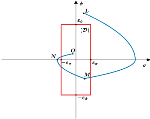
By this way, the convergence of the system trajectories to D (see Fig. 1) such that
D = {(σ, ˙σ) | |σ| ≤ εσ∧ | ˙σ| ≤ |εσ˙|} (19) is ensured, in finite time.
3∧: The notation is used for the logical AND operator.
- γ is an indicator of the accuracy of the system: if (σ, ˙σ) ∈ D, it means that the desired accuracy is reached. Then, γ = k: α increases towards 1 to reduce the energy consumption.
- If σ or ˙σ is outside ]−εσ, εσ[ or ]−εσ˙, εσ˙[ respectively, it means that the desired accuracy is not reached, hence γ = −k: α decreases towards zero in order to increase the accuracy of the system.
- If both variables are outside of their target intervals then the rate by which α decreases towards zero is three times faster (γ = −3k) to increase the accuracy faster.
Theorem 1: Consider system (1) with Assumption A1, A2 and A3 fulfilled. Then, there exist positive parameters k, εσ and εσ˙ such that ∀x(0) ∈ X , the trajectory of system (1) converges to a vicinity of the origin via the controller (16)-(17)-(18) with gains k1 and k2 tuned as in (9).
Proof:Initially, the twisting algorithm is applied α(0) = 0. As mentioned in Section II, the system trajectories will con-verge in a finite time towards the origin (see (7)). Therefore, it is guaranteed that the system trajectories converge to D in a finite time (trajectory between L and M in Fig. 1). Then, following the adaptation law, the value of α increases in order to reduce the energy consumption, unfortunately, it makes the controller less robust. By a general point-of-view, the perturbation could make the trajectory of the system leave D (point M to point N ). Therefore, α decreases again making the controller more robust: as a consequence, the trajectory comes back to D (point N to point O) and so on.
The trajectory of the system potentially goes out from D due to the perturbation, but one can be sure that it will converge back to it in finite time. Consider the worst case where α should decrease from 1 to 0 in order to bring the trajectory of the system back to D. This happens in finite time (1ks): when the twisting algorithm is applied, the trajectory converges to D in finite time too. Hence, the greater the value of k, the faster the trajectory converges.
Note that by a practical point-of-view, the twisting algo-rithm forces the trajectories to reach Sr(8). It means that, if one wants to get an efficient adaptation of α, εσ and εσ˙ have to be chosen greater than µτ2 and µτ respectively. Otherwise, a risk is to have the twisting algorithm all the time.
B. Proposition 2
In this section, a similar adaptive law is proposed but with an additional term that takes into account the control effort. γ = k(−1 + sign(εσ− |σ|) + sign(εσ˙ − | ˙σ|)) + β
|u| |u| + εu
(20) where k, β, εσ, εσ˙ and εu are positive constants. Controller (20) follows a similar logic as controller (16)-(17)-(18) presented in Section III-A; its logic can be summarized in the sequel.
σ ˙ σ • • • • ε˙σ −ε˙σ εσ −εσ (D) • • • • L M N O σ ˙ σ • • • • ε˙σ −ε˙σ εσ −εσ (D) • • • • L M N O
Fig. 1. Example of a trajectory of the system in the phase plan (σ, ˙σ) Remarks
- εσ and εσ˙ are linked to the accuracy of the controller and εu is used as a scaling factor for the normalization of the controller effort |u|.
- When the trajectories of the system are inside D, γ = k +β|u|+εu|u| : α increases towards 1 to reduce the energy consumption.
- γ in this case has two terms: the first one (−k or −3k) increases the robustness of the system and brings back the trajectories to D by decreasing α. The second term (β|u|+εu|u| ) decreases the energy consumption by increasing α when the energy consumption is high; - this means that this controller even when the trajectory
of the system is outside D, not only shall increase the robustness of the system but also shall also take into account the energy consumption. This will help to further decrease the energy consumption of the overall controller.
- Hence, β is tuned such that β < k in order to obtain the behavior described above. Otherwise, one risks to have γ positive all the time and ultimately a linear controller.
Theorem 2: Consider system (1) with Assumption A1, A2 and A3 fulfilled. Then, there exist positive parameters k, β, εσ, εσ˙ and εu such that ∀x(0) ∈ X , the trajectory of system (1) converges to a vicinity of the origin via the controller (16)-(17)-(20) with gains k1 and k2 tuned as in (9).
The proof of this theorem is similar to that Theorem 1 with one difference. The maximum finite time needed for α to decrease from 1 to 0 in order to bring back the trajectories of the system to D is k−β1 s.
IV. SIMULATIONRESULTS A. Context
Simulations have as objective to show the effectiveness of the proposed controller with the two previously exposed expressions for γ. The performances are compared to those of the twisting controller and the linear state feedback. The
software used is Simulink; the sampling period is taken 0.1 ms with Euler integration solver. The simulation time is 6 s.
The functions a(x, t) and b(x, t) are generated for 3 s using the MATLAB function ’rand’ and are taken the same while testing all controllers. For the second part of the simulation (3 s ≤ t ≤ 6 s), the sequences for a(x, t) and b(x, t) are repeated but with a different amplitude for a(x, t) such that ∀t ∈ [0, 3]
a(x, t + 3) = 4 · a(x, t)
b(x, t + 3) = b(x, t) (21) This is done in order to show the effect of the amplitude of the perturbation on the controller and the system accuracy. The bounds of these functions are (see Fig. 2)
aM = 7, bm= 0.95 and bM = 1.05 0 1 2 3 4 5 6 -7 -3.5 0 3.5 7 a ( x , t) 0 1 2 3 4 5 6 0.95 1 1.05 b ( x , t)
Fig. 2. Functions a(x, t) (top) and b(x, t) (bottom) versus time (s). The gains are stated as k1 = 30 and k2 = 10 for all controllers satisfying condition (9). The parameters for controller (16)-(17)-(18) are set as follows
k = 10, εσ= 10−5 and εσ˙ = 10−2.
whereas the parameters of controller (16)-(17)-(20) read as k = 10, β = 5, εσ= 10−5, εu= 2
and εσ˙ = 10−2. B. Results
The results are shown in Fig. 3, 4, 5, 6, 7 and 8 and some indicators are presented in Table I.
With controllers (16)-(17)-(18) and (16)-(17)-(20), the twist-ingalgorithm (α = 0) is initially applied (see Fig. 3 and 5). When the system converges (t ' 0.5 s), the adaptation begins (this phase will be called the steady state). Effective analysis of the performances is achieved on the intervals t ∈ [1, 3] and t ∈ [4, 6] where the shape of the a(x, t) is the same but with a different amplitude (see (21)).
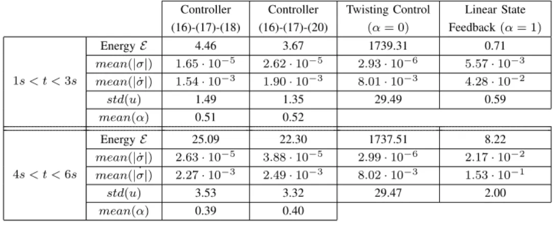
The energy consumed by the two proposed controllers is much less than that of the twisting algorithm and comparable to that of the linear state feedback (see E in Table I). The
0 1 2 3 4 5 6 0 0.5 1 α 0 1 2 3 4 5 6 -40 -20 0 20 40 u
Fig. 3. Controller (16)-(17)-(18). Top: Variable α versus time (s); Bottom: Control input u versus time (s).
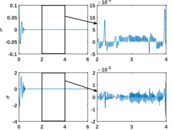
0 2 4 6 -0.1 -0.05 0 0.05 0.1 σ 2 3 4 -5 0 5 10 15×10 -5 0 2 4 6 -4 -2 0 2 ˙σ 2 3 4 -2 -1 0 1 2×10 -2
Fig. 4. Controller (16)-(17)-(18) Top: σ (with zoom) versus time (s); Bottom: ˙σ (with zoom) versus time (s).
average accuracy of |σ| (see mean(|σ|) in Table I) with both proposed controllers is higher than with the linear state feedback and comparable to the twisting algorithm, whereas the average accuracy of | ˙σ| (see mean(| ˙σ|) in Table I) with the proposed controllers is better than the other cases (concerning the twisting algorithm, this is mainly due to the attenuation of the chattering effect).
An indicator used to quantify the chattering effect is the standard deviation of the control input std(u) (see Table I): the standard deviation of the proposed controllers is significantly less than that of the twisting algorithm and slightly greater than that of the linear state feedback. This can also be seen on the control input signals of both controllers (Fig. 3 and 5) compared to the twisting controller (Fig. 7) and linear state feedback (Fig. 8). Less chattering for the proposed controllers is also manifested in Fig. 4 and 6 compared to the twisting controller 7.
When the amplitude of the perturbation/uncertainty a(x, t) is high (4 s < t < 6 s) the proposed controllers consume more energy than when a(x, t) is low (1 s < t < 3 s) (see E in Table I) since more control effort is needed to constrain the trajectories to a vicinity of the origin. Notice also that the average value of α decreases (see Table I) when a(x, t) increases making the controller more robust and potentially
0 1 2 3 4 5 6 0 0.5 1 α 0 1 2 3 4 5 6 -40 -20 0 20 40 u
Fig. 5. Controller (16)-(17)-(20) Top: Variable α versus time (s); Bottom: Control input u versus time (s).
0 2 4 6 -0.1 -0.05 0 0.05 0.1 σ 2 3 4 -4 -2 0 2 4×10 -4 0 2 4 6 -4 -2 0 2 ˙σ 2 3 4 -4 -2 0 2×10 -2
Fig. 6. Controller (16)-(17)-(20) Top: σ (with zoom) versus time (s); Bottom: ˙σ (with zoom) versus time (s).
more energy consuming.
As for the comparison between controllers (16)-(17)-(18) and (16)-(17)-(20), with the same parameters k, εσ and εσ˙, the latter is less energy consuming since it contains a term that favors energy consumption (see E in Table I), but it is less precise (see mean(|σ|) and mean(| ˙σ|) in Table I). This is due to the fact that controller (16)-(17)-(20) takes into account the energy consumption even when the accuracy is low (the trajectory is outside (D)).
V. CONCLUSION
A new controller has been proposed combining advantages of the linear state feedback and twisting controller. Low-energy consumption and high accuracy are taken into account by making variable the parameter α on the exponent terms of the proposed controller. Simulation results show the effectiveness of the proposed controller.
Future works will be dedicated to evaluate the performances of the controller applied to a real perturbed system.
Controller (16)-(17)-(18) Controller (16)-(17)-(20) Twisting Control (α = 0) Linear State Feedback (α = 1) 1s < t < 3s Energy E 4.46 3.67 1739.31 0.71 mean(|σ|) 1.65 · 10−5 2.62 · 10−5 2.93 · 10−6 5.57 · 10−3 mean(| ˙σ|) 1.54 · 10−3 1.90 · 10−3 8.01 · 10−3 4.28 · 10−2 std(u) 1.49 1.35 29.49 0.59 mean(α) 0.51 0.52 4s < t < 6s Energy E 25.09 22.30 1737.51 8.22 mean(| ˙σ|) 2.63 · 10−5 3.88 · 10−5 2.99 · 10−6 2.17 · 10−2 mean( ˙|σ|) 2.27 · 10−3 2.49 · 10−3 8.02 · 10−3 1.53 · 10−1 std(u) 3.53 3.32 29.47 2.00 mean(α) 0.39 0.40 TABLE I
ENERGY CONSUMPTION,AVERAGE ACCURACY ONσANDσ,˙ STANDARD DEVIATION OFu (std(u))AND AVERAGE VALUE OFαIN STEADY STATE WITH CONTROLLER(16)-(17)-(18),CONTROLLER(16)-(17)-(20), twistingCONTROLLER AND LINEAR STATE FEEDBACK FOR1s < t < 3sAND4s < t < 6s
0 1 2 3 4 5 6 -50 0 50 u 0 2 4 6 -0.1 0 0.1 σ 2 3 4 -1 0 1×10 -5 0 2 4 6 -5 0 5 ˙σ 2 3 4 -5 0 5×10 -2
Fig. 7. Twisting controller (from top to bottom) Control input u, σ and ˙
σ versus time (s).
REFERENCES
[1] E. Bernuau, D. Efimov, W. Perruquetti and A. Polyakov “On homo-geneity and its application in sliding mode control.” Journal of the Franklin Institute 351.4 (2014): 1866-1901.
[2] S.P. Bhat and D.S. Bernstein. “Finite-time stability of homogeneous systems.” In American Control Conference, Albuquerque, New Mex-ico, United States (1997).
[3] C. Edwards and Y. Shtessel. “Adaptive continuous higher order sliding mode control.” Automatica 65 (2016): 183-190.
[4] M. Gopal. Control systems: principles and design. Tata McGraw-Hill Education (2002).
[5] S. Laghrouche, M. Smaoui, F. Plestan and X. Brun “Higher order slid-ing mode control based on optimal approach of an electropneumatic actuator.” International Journal of Control 79.2 (2006): 119-131. [6] S. Laghrouche, F. Plestan and A. Glumineau. “Higher order sliding
mode control based on integral sliding mode.” Automatica 43.3 (2007): 531-537.
[7] A. Levant. “Sliding order and sliding accuracy in sliding mode control.” International Journal of Control 58.6 (1993): 1247-1263. [8] A. Levant. “Universal single-input-single-output (SISO) sliding-mode
controllers with finite-time convergence.” IEEE transactions on Auto-matic Control 46.9 (2001): 1447-1451.
[9] A. Levant. “Homogeneity approach to high-order sliding mode de-sign.” Automatica 41.5 (2005): 823-830.
[10] W. Perruquetti and T. Floquet. “Homogeneous finite time observer for nonlinear systems with linearizable error dynamics.” In IEEE Conference on Decision and Control, New Orleans, Louisiana, United States (2007). 0 1 2 3 4 5 6 -10 0 10 u 0 1 2 3 4 5 6 -0.2 0 0.2 σ 0 1 2 3 4 5 6 -1 0 1 ˙σ
Fig. 8. Linear state feedback (from top to bottom) Control input u, σ and ˙σ versus time (s).
[11] F. Plestan, Y. Shtessel, V. Bregeault and A. Poznyak. “New method-ologies for adaptive sliding mode control.” International Journal of Control 83.9 (2010): 1907-1919.
[12] V.G. Rao and D.S. Bernstein. “Naive control of the double integrator.” IEEE Control Systems Magazine 21.5 (2001): 86-97.
[13] T. S`anchez, and J.A. Moreno. “Construction of lyapunov functions for a class of higher order sliding modes algorithms.” In IEEE Conference on Decision and Control, Atlanta, Georgia, USA (2012).
[14] Y. Shtessel, C. Edwards, L. Fridman and A. Levant. Sliding mode control and observation. New York, NY, USA: Birkh¨auser (2014). [15] Y. Shtessel, J.A. Moreno, F. Plestan, L.M. Fridman and A.S. Poznyak.
“Super-twisting adaptive sliding mode control: A Lyapunov design.” In IEEE Conference on Decision and Control, Atlanta, Georgia, USA (2010).
[16] Y. Shtessel, M. Taleb and F. Plestan. “A novel adaptive-gain su-pertwisting sliding mode controller: Methodology and application.” Automatica 48.5 (2012): 759-769.
[17] V.I. Utkin. Sliding modes in control and optimization. Springer Sci-ence and Business Media (2013).