HAL Id: inria-00069876
https://hal.inria.fr/inria-00069876
Submitted on 19 May 2006
HAL is a multi-disciplinary open access
archive for the deposit and dissemination of
sci-entific research documents, whether they are
pub-lished or not. The documents may come from
teaching and research institutions in France or
abroad, or from public or private research centers.
L’archive ouverte pluridisciplinaire HAL, est
destinée au dépôt et à la diffusion de documents
scientifiques de niveau recherche, publiés ou non,
émanant des établissements d’enseignement et de
recherche français ou étrangers, des laboratoires
publics ou privés.
Smaller Connected Dominating Sets in Ad Hoc and
Sensor Networks based on Coverage by Two-Hop
Neighbors
François Ingelrest, David Simplot-Ryl, Ivan Stojmenovic
To cite this version:
François Ingelrest, David Simplot-Ryl, Ivan Stojmenovic. Smaller Connected Dominating Sets in Ad
Hoc and Sensor Networks based on Coverage by Two-Hop Neighbors. [Research Report] RT-0304,
INRIA. 2005, pp.12. �inria-00069876�
ISSN 0249-0803
a p p o r t
t e c h n i q u e
Thème COM
INSTITUT NATIONAL DE RECHERCHE EN INFORMATIQUE ET EN AUTOMATIQUE
Smaller Connected Dominating Sets
in Ad Hoc and Sensor Networks
based on Coverage by Two-Hop Neighbors
François Ingelrest — David Simplot-Ryl — Ivan Stojmenovi´c
N° 0304
Unité de recherche INRIA Futurs Parc Club Orsay Université, ZAC des Vignes, 4, rue Jacques Monod, 91893 ORSAY Cedex (France)
Téléphone : +33 1 72 92 59 00 — Télécopie : +33 1 72 92 59 ??
Smaller Connected Dominating Sets
in Ad Hoc and Sensor Networks
based on Coverage by Two-Hop Neighbors
François Ingelrest
∗, David Simplot-Ryl
∗, Ivan Stojmenović
†Thème COM — Systèmes communicants Projet POPS
Rapport technique n° 0304 — Avril 2005 — 12 pages
Abstract: In this paper, we focus on the construction of an efficient dominating set in ad hoc and sensor networks. A set of nodes is said to be dominating if each node is either itself dominant or neighbor of a dominant node. This set can for example be used for broadcasting, so the smaller the set is, the more efficient it is. As a basis for our work, we use a heuristics given by Dai and Wu for constructing such a set and propose an enhanced definition to obtain smaller sets. This approach, in conjunction with the elimination of message overhead by Stojmenović, has been shown (in recent studies) to be an excellent compromise with respect to a wide range of metrics considered. In our new definition, a node u is not dominant if there exists in its 2-hop neighborhood a connected set of nodes with higher priorities that covers u and its 1-hop neighbors. This new rule uses the exact same level of information required by the original heuristics, only neighbors of nodes and neighbors of neighbors must be known to apply it, but it takes advantage of some knowledge originally not taken into account: 1-hop neighbors can be covered by some 2-hop neighbors. We give the proof that the set obtained with this new definition is a subset of the one obtained with Dai and Wu’s heuristics. We also give the proof that our set is always dominating for any graph, and connected for any connected graph. Two versions were considered: with topological and positional information, which differ in whether or not nodes are aware of links between their 2-hop neighbors that are not 1-hop neighbors. An algorithm for applying the concept at each node is described. We finally provide experimental data that demonstrates the superiority of our rule in obtaining smaller dominating sets. A centralized algorithm was used as a benchmark in the comparison. The overhead of the size of connected dominating set was reduced by about 15% with the topological variant and by about 30% with the positional variant of our new definition.
Key-words: Ad Hoc Networks, Sensor Networks, Connected Dominating Sets, Local Heuristics, Broadcasting.
∗IRCICA/LIFL, Univ. Lille 1, INRIA futurs, France. Email: {Francois.Ingelrest, David.Simplot}@lifl.fr † Computer Science, SITE, University of Ottawa, Ontario K1N 6N5, Canada. Email: [email protected]
Petits ensembles dominants connexes
basés sur la couverture des voisins à deux sauts
pour réseaux ad hoc et de capteurs.
Résumé : Dans cet article, nous nous intéressons à la construction d’un ensemble dominant efficace pour les réseaux ad hoc et de capteurs. Un ensemble est qualifié de dominant si chaque nœud est lui-même dominant ou voisin direct d’un nœud dominant. Un tel ensemble pouvant par exemple être utilisé pour faire de la diffusion d’informations, plus il sera petit, plus il sera efficace. Notre travail se base sur une heuristique donnée par Dai et Wu permettant de construire un tel ensemble et propose une définition améliorée afin d’obtenir de plus petits ensembles. Cette approche, utilisée avec l’élimination du surplus de messages par Stojmenović, a été récemment démontrée comme étant un excellent compromis vis-à-vis d’une large gamme de métriques. Dans notre définition, un nœud u n’est pas dominant s’il existe dans son voisinage à 2 sauts un ensemble connexe de nœuds de plus haute priorité qui couvre u et son voisinage à 1 saut. Cette nouvelle règle nécessite les mêmes informations que celles de l’heuristique originale, seule la connaissance des voisins des nœuds et les voisins de ces voisins est nécessaire pour pouvoir l’appliquer, mais elle tire partie d’informations originellement non prises en compte: les voisins à 1 saut peuvent être couverts par des voisins à 2 sauts. Nous fournissons la preuve que l’ensemble obtenu avec cette nouvelle définition est un sous-ensemble de celui obtenu avec l’heuristique de Dai et Wu. Nous donnons également la preuve que notre ensemble est toujours dominant pour n’importe quel graphe, et toujours connexe pour n’importe quel graphe connexe. Deux versions sont considérées: avec des informations topologiques ou de position, ces deux versions différant dans le fait que les nœuds connaissent ou non les liens entre leurs voisins à 2 sauts. Un algorithme permettant d’appliquer cette nouvelle règle au niveau de chaque nœud est décrite. Finalement, nous fournissons des résultats expérimentaux qui démontrent la supériorité de notre règle dans l’obtention d’ensembles dominants plus petits. Un algorithme centralisé est utilisé comme référence dans ces comparaisons. Le surcoût de la taille de l’ensemble dominant connexe est réduit d’environ 15% avec la variante topologique tandis qu’elle est réduite de près de 30% avec la variante positionnelle. Mots-clés : Réseaux ad hoc, Réseaux de capteurs, Ensembles dominants connexes, Heuristique locale, Diffusion d’informations.
Smaller CDS for Ad Hoc and Sensor Networks 3
1
Introduction
Wireless networking has become an essential part of new technologies, allowing nomadic users to keep in touch with their family or their office using miscellaneous devices such as laptops, PDA’s or smartphones. The most deployed technology, known as WiFi, is still very restrictive as users must be within the range of a correctly configured access point. Densely populated area like airports or train stations can easily be equipped with needed infrastructure, but it is not the case for other areas, where multi-hop wireless links may be desirable. Multi-hop wireless ad hoc and sensor networks have been widely studied recently. They are composed of a set of hosts operating in a self-organized and decentralized manner, which can communicate together using a radio interface. As in any wireless network, transmission ranges are limited due to propagation path loss, health and energy considerations. Thus, each node must act alternately as a terminal and a router, depending on the needs of the system, leading to a cooperative multi-hop routing.
Energy conservation is one of the most challenging problems in ad hoc and sensor networks because batteries have very limited capacities. Two particular important problems are activity scheduling and broadcasting. In activity scheduling problem, some nodes decide to sleep to preserve the energy, but should have an active neighbor to collect messages for them or take over some sensing tasks. In broadcasting problem, one host needs to send a particular message to all the other ones in the network. Broadcasting is applied for route discovery [6], publication of services, alarming and other operations. In a straightforward solution to broadcasting, hosts only need to blindly relay packets at least once to their neighborhood. However, this leads to the well-known broadcast storm problem [8]. While consuming a lot of energy, this method does not even ensure a complete coverage of the network due to multiple collisions.
In a connected dominating set (CDS), each node either belongs to CDS or has a (1-hop) neighboring node in CDS. In an activity scheduling solution, only nodes from CDS may remain active. To reduce the set of relaying nodes in a broadcasting task, only nodes marked as dominant have to act as routers to relay the broadcasting packet, so that the broadcasting is performed by retransmitting by as few nodes as possible. An efficient distributed algorithm, known as the generalized self-pruning rule [3], has been proposed to compute CDS by using only local information. In this paper, we propose an improvement to this rule: by using exactly the same local information at each node, our new rule elects fewer nodes as dominant. No additional message exchanges are required to apply it, and needed information can be obtained using simple beacon messages. We also give the theoretical proof that the set of nodes elected by our algorithm is always dominant and connected, and provide experimental data demonstrating the superiority of our method.
The remainder of this paper is organized as follows: in the next section, we provide the definitions needed by our network model, while in Sec. 3 a review of the existing works is proposed. In Sec. 4 we describe our algorithm and give the proof that the designated set is indeed always dominant and connected. We then provide in Sec. 5 experimental data for our new method and comparisons with existing work. We finally conclude in Sec. 6 and give some directions for future work.
2
Preliminaries
The common representation of a wireless network is a graph G = (V, E), where V is the set of vertices (the hosts, or nodes) and E ⊆ V2 the set of edges which represent the available communications: if a node v is a physical neighbor of a node u (v is within the communication range of u and thus receives its messages), then there exists (u, v) ∈ E. If we assume that all nodes have the same communication radius, denoted by R, then the set E is defined by:
E = {(u, v) ∈ V2| d(u, v) ≤ R},
d(u, v) being the Euclidean distance between nodes u and v. Each node u must be assigned a unique identifier id(u) (this can be, for instance, IP or MAC address). We define the neighborhood set N (u) of a node u as:
N (u) = {v ∈ V | v 6= u ∧ (u, v) ∈ E}, and the extended neighborhood set ˙N (u) as:
˙
N (u) = N (u) ∪ {u}.
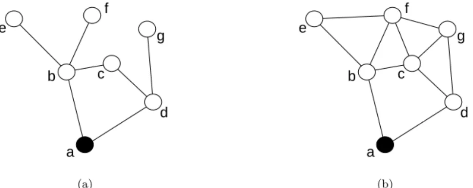
4 Ingelrest & Simplot-Ryl & Stojmenović b d a c e f g (a) b d a c e f g (b)
Figure 1: Topological information vs. positional information.
The neighborhood function is naturally extended to sets of nodes: for a given subset V0
of V , we have N (V0
) =S
u∈V0N (u). The degree of a node u is simply its number of neighbors |N (u)|, while the density of
the network is the average size of the extended neighborhood sets. We measure the distance between two nodes u and v in terms of number of hops, which is simply the minimum number of edges a message has to cross to travel from u to v.
A graph GD= (VD, ED), where VD⊆ V and ED ⊆ E, is dominant iff: ∀u ∈ V ∃v ∈ VD| u ∈ ˙N(v).
In simple terms, each vertex is either dominant or 1-hop neighbor of a dominant one. The set ED is the subset of E that contains only edges between two dominant neighbors:
ED= {(u, v) ∈ VD2 | d(u, v) ≤ R}.
We assume that each node is aware of its 2-hop neighbors. This is achieved in two rounds of HELLO messages. First, each node informs its neighbors about its existence (and position, if this information is available). Next, each node sends message to all its neighbors informing about its 1-hop neighbors (nodes from which HELLO message in the first round was received). In a mobile ad hoc network, each node (regularly or based on its mobility) emits additional HELLO messages, to maintain 2-hop information. When a node u receives from a node v such a message, u adds v to its neighborhood table, or updates the entry if it was already there. Too old entries are regularly removed from the table, as corresponding nodes have not signaled themselves recently. If the distances between neighbors are needed, the easiest method to obtain them is to have nodes add their position in their beacon messages. Positions can simply be acquired by using a location system like the GPS (Global Positioning System). Other methods can be used, like deducing distances to neighbors by measuring the reception power of messages. In the graph representing the 2-hop knowledge at each node, there exists a difference between topological and positional information that may be used. If position information is available, each node may conclude, based on their locations, whether or not two of its 2-hop neighbors (which are not 1-hop neighbors) are neighbors themselves. Such a conclusion cannot be made without position information (that is, based solely on topological information), and therefore no edge between such neighbors is assumed. Fig. 1 illustrates the difference between these two assumptions, considering node a. With topological information, in 1(a), the 2-hop neighbors {c, e, f, g} are assumed to not be directly connected, while it is not the case with positional information in 1(b). However, node c is always known to be a common neighbor of nodes b and d because it appears in both neighborhood lists.
3
Related Work
As stated in Sec. 1, the easiest method for broadcasting a packet is to have all nodes act as routers and relay it at least once to their neighborhood: this method is known as blind flooding. However, such a simple behavior has huge drawbacks: too many packets are lost due to collisions between neighboring nodes (this can lead to only a partial coverage of the network) and far too much energy is consumed.
Smaller CDS for Ad Hoc and Sensor Networks 5 a b c d e f g
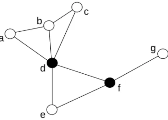
Figure 2: A dominating set composed of nodes {d, f }.
A possible method to reduce the energy consumption is to determine a set of nodes, such that if only those nodes act as routers, the broadcasting is still achieved. A dominating set of vertices VD is suitable for this task, as long as it is connected (there exists a path in GD between any two vertices). Once such a set has been obtained, the broadcasting process becomes obvious:
• The source node sends the packet to its neighborhood,
• Each dominant node that receives it act as a router and relays it to its neighbors, • Each non-dominant node simply drops it.
Besides this simple method, dominating sets can also be used as part of a more sophisticated broadcasting mechanisms [5].
The simplest connected dominating set is the unit graph itself, and using such a set for broadcasting is the same as performing a blind flooding. The problem of computing the smallest possible connected dominating set is known to be a NP-complete problem and requires a global knowledge of the network topology, thus many centralized and distributed approximated algorithms for constructing efficient sets have been proposed. We will describe only one here, which is quite simple, efficient compared to others, and easy to describe. It is a centralized algorithm proposed by Guha and Khuller in [4] as follows. Each node is initially colored as white. The densest node in the graph is then colored as black, and all its neighbors as grey nodes. Then, iteratively, while there exists some white nodes, the grey node with the largest number of white neighbors is selected, colored as black node, and all its white neighbors as grey nodes. Ties can be resolved by using some keys (identifiers). At the end, the set of black nodes is a connected dominating set, and its size is a good estimate of the limits one can reach with a localized heuristics. Some localized efficient heuristics have also been proposed and can thus be applied in ad hoc networks.
Wu and Li proposed in [14] an algorithm that has been later improved in term of message overhead in [12,11]. We describe here the latter because it requires no messages once 2-hop neighborhood information is available. A node is referred to as intermediate if it has at least two neighbors not directly connected. A node u is covered by a node v ∈ N (u) if N (u) ⊆ N (v) and key(v) > key(u). Nodes that are not covered by any neighbor are called inter-gateway nodes. A node u is covered by two connected nodes v ∈ N (u) and w ∈ N (u) if N (u) ⊆ (N (v) ∪ N (w)), key(v) > key(u) and key(w) > key(u). Inter-gateway nodes that are not covered by any pair of connected neighboring nodes become gateway nodes.
This rule has been further improved in term of number of dominating nodes by Dai and Wu [3]: they proposed a more general rule where coverage can be provided by an arbitrary number of connected 1-hop neighbors. A modification of this generalized self-pruning rule has been proposed by Stojmenović in [13] in order to avoid similar message exchanges between neighbors. A node u is covered by a set of 1-hop neighbors Au if Au is connected, N (u) ⊆ N (Au) and if each node in Auhas a higher key than u. It has been further computationally simplified by Carle and Simplot-Ryl [2] as follows. First, each node checks if it is intermediate, that is, whether it has at least two neighbors not directly connected. Then each intermediate node u constructs a subgraph Gh of its 1-hop neighbors with higher keys. In the graph composed by N (u), each node which has a lower key than u is removed, as well as the corresponding edges. The resulting subgraph is denoted by Gh. If the latter is empty or disconnected then u is in the dominating set. If Ghis connected but there exists a neighbor of u which is not neighbor of any node from Ghthen u is in the dominating set. Otherwise u is covered and is not in the
6 Ingelrest & Simplot-Ryl & Stojmenović d c a b e f g (a) d c a b e f g (b)
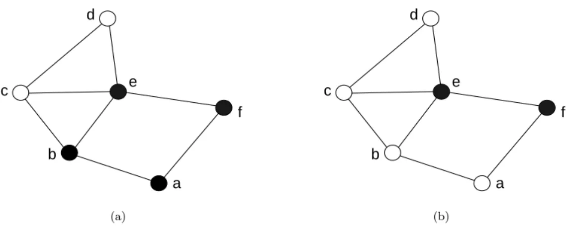
Figure 3: Different priorities lead to different dominating sets.
dominating set. Dijkstra’s shortest path algorithm can be used to test the connectivity (it is performed locally at each node). Non-intermediate nodes are never dominant. This rule is illustrated by Fig. 2, where black nodes are dominant, and identifiers of nodes are used as keys using the alphabetical order for comparisons. Nodes {a, c, e, g} are not intermediate because they do not have unconnected neighbors, they are thus not dominant. Node b has two unconnected neighbors {a, c}, but it also has a neighbor d with a higher key that covers {a, b, c}, so b marks itself as not dominant. Only nodes {d, f } are not covered by the generalized rule, and thus mark themselves as dominant.
The key of a node represents its priority, and it is assumed to be unique for each node. A simple priority can be the identifier of the node, but it can also be any collection of values with the aim of increasing the efficiency of the dominating set. For example, in [15] the proposed key for a node u is:
key(u) = {energy(u), degree(u), id(u)}.
This means that nodes with higher energy level have a larger probability to be elected as dominant. If the energy levels are equal for two nodes, then the second key, degree, is used for comparison. Finally, if there is a tie with the degree as well, the identifier is used. Fig. 3 illustrates the differences obtained when using different sort of keys: in 3(a), the keys are the identifiers of nodes, while in 3(b) the degree is used a the primary key and the identifier as the secondary one. Some other keys were later proposed and studied in [10].
Liu et al. recently proposed in [7] an iterative localized algorithm for connected dominating sets, improving the concept of [14] in terms of size of conencted dominating sets, but at the expense of additional messages between neighboring nodes. The principle is to have nodes exchange messages with their neighbors (there are exactly 5 messages exchanged) in order to decide whether they should be dominant, using information received from their neighbors. At each step, each node that decides not to be dominant becomes passive; otherwise it is active and reevaluates this decision in the next round. There can be 6 messages exchanged if each node wants to know which of its neighbors are dominant. The authors claimed that this process prevents ‘illegal simultaneous’ removals from the dominating set, which may disconnect it. The experimental performances show that the computed set is efficient, but the communication overhead and the synchronization needed make it more difficult to apply in a distributed environment. Furthermore, beacon messages are also needed for the first step to take place.
In [1], Basagni et al. proposed a performance comparison of various protocols for computing backbones in ad hoc networks, including the previously cited protocols. They measured miscellaneous parameters, like the computation complexity (needed time to create the backbone), the backbone size or even the energy consumption per node in order to determine which protocol suits the best to ad hoc networks. They concluded that Wu and Li’s algorithm used in conjunction with the variant by Stojmenović et al. [12] is an excellent compromise with respect to all the considered metrics, and overall far superior than any other approach that exists in literature. This study completely justifies our approach on working on this concept to propose a more efficient one.
Smaller CDS for Ad Hoc and Sensor Networks 7 b e a f c d (a) b e a f c d (b)
Figure 4: The generalized self-pruning rule and its improvement.
4
Dominating sets based on coverage by two-hop neighbors
In this section, we give the new definition for computing a connected dominating set over a connected graph by using 2-hop topological or positional information. We also provide proofs that the set obtained with this new definition:
• is a subset of the one obtained with Dai and Wu’s heuristics, • is always dominating for any graph,
• is always connected for any connected graph.
We also provide an efficient algorithm to apply this rule in a practical environment.
4.1
Description
Our new definition of dominating sets is based on the observation that the method used by Dai and Wu [3] requires 2-hop topological knowledge, because nodes need to know their neighbors and the neighbors of their neighbors, and that this knowledge could be better used by applying some enhanced concepts. To illustrate this, let us consider Fig. 4(a) where the generalized self pruning rule has been applied using the alphabetical order to determine the priority of the node. The node a has been marked as dominant because it has two neighbors {b, f } not covered by any set of neighbors with higher priority. In fact, a is itself covered by {b, e, f } although e is not a 1-hop neighbor, and a could be marked as passive as illustrated in 4(b): the set of black nodes would remain connected and dominant. While e is not a direct neighbor of a, this does not prevent the latter from verifying whether any of its neighbors are neighbors of e, or whether b, e and f are connected, since e appears in the list of neighbors sent to a by its 1-hop neighbors, therefore such conclusion can be made. Similarly in 4(b), node b concludes that it is not dominant since all its neighbors {a, c, e} and itself are covered by its connected higher key 2-hop neighbors e, f.
Therefore, our new definition of the dominating set VD can de described as follows:
∀u ∈ V u /∈ VD⇔ (1)
∃Au⊆ ˙N (u)2\ {u} ∀v ∈ Au, key(v) > key(u) Auconnected ˙ N (u) ⊆ ˙N (Au)
In other words, a node u is covered (and thus not dominant) if there exists in its 2-hop neighborhood a connected set of nodes with higher priorities which covers ˙N (u). Note that, when topological information is used, u is not aware of possible links between its 2-hop neighbors, and therefore may declare the set disconnected although in reality it may be connected (refer to Fig. 1). This can be avoided if nodes are able to determine their location: they can add it to their beacon messages, and thus links between 2-hop neighbors will be part of the knowledge of nodes. This variant is considered from an experimental point of view in Sec. 5.
8 Ingelrest & Simplot-Ryl & Stojmenović
A
uv
u
w
v’
w’
Figure 5: Removal of vertex u does not lead to a loss of connectivity between v and w.
4.2
Proof of inclusion
Theorem 1: The dominating set VD computed with our new definition is a subset of the one obtained with the generalized self-pruning rule.
Proof: In the generalized self-pruning rule, a node u is marked as not dominant if there exists a connected subset of N (u) composed by higher priority neighbors such that ˙N (u) is covered by this subset. As N (u) ⊆
˙
N (u)2\ {u}, if there exists such a set in N (u), then it also exists in ˙N (u)2\ {u}. We can thus deduce that nodes marked as not dominant by the generalized self-pruning rule are also marked as not dominant by our new definition, which can only remove more nodes from the dominating set.
This proof demonstrates that our new definition cannot generate a larger set VDthan the one obtained with the generalized self-prunning rule.
4.3
Proof of dominance
Theorem 2: For any given graph G = (V, E), each node u ∈ V either belongs to VD or is a neighbor of a node v ∈ VD.
Proof: Assume that the set VDis not dominating. Let u be a node which is not in the dominating set and has no dominant neighbor. Node u is covered by Au, set of 2-hop neighbors with higher key values than u. Let v be the node with the highest key value in N (u). Node v has higher priority than u because of the existence of Au and the need for at least one node from Au to be 1-hop neighbor of u. Node v is not dominant because u is not covered by VD. It is thus covered by a set Av. Therefore u is neighbor of a node w from Av. Node w is therefore neighbor of u and has higher key value than v, which is a contradiction with respect to the choice of v.
4.4
Proof of connectivity
Theorem 3: For any given connected graph G = (V, E), there exists a path between any two vertices in the graph GD= (VD, ED) produced by our algorithm.
Proof: We may assume that nodes are removed one by one in ascending order of priority instead of simultaneous removal and will show that the removal of any node u preserves the connectivity. Let vuw be a path via node u. Node u is removed because of the set Au, which is connected and covers its neighbors, as illustrated by Fig. 5. Moreover, no nodes of Auhas already been removed since Aucontains nodes with higher priority than u. This means that there are two nodes v0
and w0
from Auso that v is neighbor of v0, w is neighbor of w0
, and v0 and w0
are connected in Au. This means that nodes v and w remain connected after removal of node u. We can thus deduce that a node u will never ‘remove’ itself from the dominating graph if there does not exist another path between any two components that are ‘glued’ together thanks to u.
All three proofs do not depend on the possible links between 2-hop neighbors. They are therefore valid for both topological and positional information. This does not mean that they will result in the same dominating set. On the contrary, they can differ, since these ‘special’ links may be used to make a set of neighbors with higher priorities connected.
Smaller CDS for Ad Hoc and Sensor Networks 9
v
w
a
u
x
Figure 6: A new algorithm must be used for the enhanced definition.
4.5
Algorithm
It could seem at first that the algorithm used for Dai and Wu’s heuristics described in Sec. 3 could also be used for our new definition: instead of computing the graph Gh using the 1-hop neighborhood, it could be computed using the 2-hop neighborhood (minus the links between the 2-hop neighbors in case of topological information). However this may not work correctly, as illustrated by Fig. 6: node u is not dominant because there exists a connected set {v, w} which covers {a, u}. However, the set of nodes of higher priority within the 2-hop neighborhood {v, w, x} is not connected. Using the original algorithm, u would have been marked as dominant.
We therefore describe here a new algorithm for testing whether or not node u will declare itself as being in dominating set as follows:
1. Create a graph Gh composed from the nodes of higher priority than u within the 2-hop neighborhood of u.
2. Find the connected components in Gh; this can be done by repeated application of Dijkstra’s shortest path algorithm starting each time from an unseen node. Alternately, depth first search or breath first search protocols can be repeatedly applied to find all components.
3. If u and its 1-hop neighbors are covered by at least one component, then mark u as not dominant.
5
Performances Evaluation
In our simulation, we compared our enhanced definition with the original heuristics by Dai and Wu. We did not consider other methods because of their communication overhead for construction and maintenance and other significant drawbacks as verified by Basagni et al. [1]. On the other hand, only beacon (‘HELLO’) messages are required for the two compared rules. We used a very efficient centralized algorithm by Guha and Khuller [4] as the benchmark in our comparisons. That algorithm is a good measure of the ability of localized algorithms to produce small connected dominating sets, and a good indicator of progress made among localized protocols.
We use the following abbreviations: • CH: Centralized heuristics. • ED: Enhanced definition.
• EDPOS: Enhanced definition with positioning information, this means that nodes are aware of links between their 2-hop neighbors.
• GSPR: Generalized self-pruning rule.
The parameters of the simulations are the following. The network is static and always composed of 500 nodes randomly distributed in a uniform manner over a square area whose size is computed in order to obtain a given degree. We define the latter as the number of nodes in a communication area. For each measure, we took the average value obtained after 500 iterations.
10 Ingelrest & Simplot-Ryl & Stojmenović 0 5 10 15 20 25 30 35 40 45 10 20 30 40 50 60 70 80 90 100 Dominant nodes (%)
Degree (unit graph)
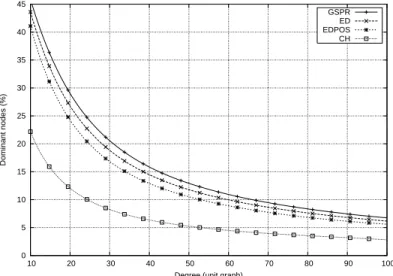
GSPR ED EDPOS CH
Figure 7: Percentage of dominant nodes for varying degree.
80 90 100 110 120 130 140 150 160 10 20 30 40 50 60 70 80 90 100 Overhead over CH (%)
Degree (unit graph)
GSPR ED EDPOS (a) 0 5 10 15 20 25 30 35 10 20 30 40 50 60 70 80 90 100
Improvement in overhead over GSPR (%)
Degree (unit graph)
ED EDPOS
(b)
Figure 8: Overhead compared to CH.
We give in Fig. 7 the average percentage of dominant nodes obtained by applying the different schemes for varying degree between 10 and 100. Not surprisingly, the centralized greedy heuristics performs the best in obtaining small dominating sets for all ranges, and for high degree like 50, only 5.15% of nodes are marked as dominant. As theoretically proven in previous section, our enhanced definition always performs better in giving smaller dominating sets in the average case. For the value of 20 nodes per communication area, only 26% of nodes are elected as dominant, against 28.19% for the generalized self-pruning rule. As expected, using positioning information brings even better results, and only 23.4% of nodes are then marked as dominant. For higher density (50) the percentage of dominant nodes even decreases down to respectively 11.56% and 10.32%. We provide in Fig. 8 the overhead of the localized heuristics over the centralized one. Considering degree 30 in 8(a), GSPR has an overhead equal to 151%: this means that this heuristics elects 151% more nodes as dominant than CH. For the same degree, ED has an overhead of 129%, this is a difference of 22%. With positioning information, EDPOS scores only an overhead of 105%, the difference being equal this time to 46%. In summary, as illustrated in 8(b), the overhead of the size of connected dominating set was reduced by about 15% with the topological variant and by about 30% with the positional variant of our new definition, with respect to the generalized self prunning rule. These percentages appears rather stable with respect to the network densities, for dense networks.
Smaller CDS for Ad Hoc and Sensor Networks 11 0 0.5 1 1.5 2 2.5 3 3.5 4 4.5 10 20 30 40 50 60 70 80 90 100 Degree (CDS)
Degree (unit graph)
GSPR ED EDPOS CH (a) 0.6 0.65 0.7 0.75 0.8 0.85 0.9 10 20 30 40 50 60 70 80 90 100
Length ratio of an edge (CDS)
Degree (unit graph)
GSPR ED EDPOS CH
(b)
Figure 9: Comparison of the produced CDS’s.
We finally give in Fig. 9 a comparison of the protocols in terms of the dominant graphs they produce. In 9(a) is given the average degree of the CDS’s (this is the average number of dominant neighbors per dominant node). Not surprisingly, this value is dependent on the average size of the CDS’s: the smallest is the set, and the smallest is the average degree, so CH obtains the best results and GSPR the highest ones. An interesting remark is that the degree of the produced CDS’s is relatively constant for varying degree of the unit graph. The degree of the localized algorithms varies between 3 and 4, while the average degree of the centralized heuristics is around 2. We also consider in 9(b) the average length of the edges between two dominant neighbors divided by R. Once again, this value is relatively stable and does not really depend on the degree of the unit graph. The three localized schemes obtain nearly the same results, while CH has higher values. This can be easily explained: in this heuristics, at each step, the node with the highest number of ‘non-covered’ neighbors is chosen, and we can expect this value to increase with the distance between the nodes.
6
Conclusion
In this paper, we have presented an enhanced definition for computing a dominating set in ad hoc networks, using as a basis a work from Dai and Wu. We have proven that our rule gives a subset of the one obtained thanks to the original algorithm. We have also proven that this subset is always dominating, and connected for any connected graph. We finally provided experimental results which demonstrate the superiority of our rule over the original one in electing fewer nodes as dominant.
Our future research includes experiments under the NS2 simulator [9] using a realistic mobility model, to be able to emphasize the gain obtained thanks to our localized heuristics when compared to an algorithm that requires additional messages exchange.
References
[1] S. Basagni, M. Mastrogiovanni, A. Panconesi, and C. Petrioli. Localized protocols for ad hoc clustering and backbone formation: A performance comparison. IEEE Transactions on Parallel and Distributed Systems, 2004. To appear.
[2] J. Carle and D. Simplot-Ryl. Energy efficient area monitoring by sensor networks. IEEE Computer Magazine, 37(2):40 – 46, 2004.
[3] F. Dai and J. Wu. Distributed dominant pruning in ad hoc networks. In Proceedings of the IEEE Interna-tional Conference on Communications (ICC’03), Anchorage, Alaska, May 2003.
[4] S. Guha and S. Khuller. Approximation algorithms for connected dominating sets. Algorithmica, 20(4):374 – 387, April 1998.
12 Ingelrest & Simplot-Ryl & Stojmenović
[5] F. Ingelrest, D. Simplot-Ryl, and I. Stojmenović. A dominating sets and target radius based localized activity scheduling and minimum energy broadcast protocol for ad hoc and sensor networks. In Proceedings of the Mediterranean Ad Hoc Networking Workshop (Med-Hoc-Net 2004), Bodrum, Turkey, June 2004. [6] D.B. Johnson, D.A. Maltz, and Y.-C. Hu. The dynamic source routing protocol for mobile ad hoc networks
(DSR). Internet Draft, draft-ietf-manet-dsr-10.txt, July 2004. Work-in-progress.
[7] H. Liu, Y. Pan, and J. Cao. An improved distributed algorithm for connected dominating sets in wireless ad hoc networks. In Proceedings of the International Symposium on Parallel and Distributed Processing and Applications (ISPA’04), Hong Kong, China, December 2004.
[8] Sze-Yao Ni, Yu-Chee Tseng, Yuh-Shyan Chen, and Jang-Ping Sheu. The broadcast storm problem in a mo-bile ad hoc network. In Proceedings of the International Conference on Momo-bile Computing and Networking (MobiCom’99), Seattle, USA, August 1999.
[9] NS2. http://www.isi.edu/nsnam/ns/.
[10] J.A. Shaikh, I.Stojmenović, and J. Wu. New metrics for dominating set based energy efficient activity scheduling in ad hoc networks. In Proceedings of the International Workshop on Wireless Local Networks (WLN 2003), Bonn, Germany, October 2003.
[11] I. Stojmenović. Comments and corrections to ‘dominating sets and neighbor elimination-based broadcasting algorithms in wireless networks’. IEEE Transactions on Parallel and Distributed Systems, 15(11):1054 – 1055, November 2004.
[12] I. Stojmenović, M. Seddigh, and J. Zunic. Dominating sets and neighbor elimination-based broadcasting algorithms in wireless networks. IEEE Transactions on Parallel and Distributed Systems, 13(1):14 – 25, January 2001.
[13] I. Stojmenović and J. Wu. Mobile Ad Hoc Networking, chapter Broadcasting and Activity Scheduling in Ad Hoc Networks, pages 205 – 229. IEEE Press, August 2004.
[14] J. Wu and H. Li. On calculating connected dominating sets for efficient routing in ad hoc wireless net-works. In Proceedings of the ACM International Workshop on Discrete Algorithms and Methods for Mobile Computing and Communications (DIALM 1999), Seattle, USA, August 1999.
[15] J. Wu, B. Wu, and I. Stojmenović. Power-aware broadcasting and activity scheduling in ad hoc wireless networks using connected dominating sets. Wireless Communications and Mobile Computing, 4(1):425 – 438, June 2003.
Unité de recherche INRIA Futurs Parc Club Orsay Université - ZAC des Vignes 4, rue Jacques Monod - 91893 ORSAY Cedex (France)
Unité de recherche INRIA Lorraine : LORIA, Technopôle de Nancy-Brabois - Campus scientifique 615, rue du Jardin Botanique - BP 101 - 54602 Villers-lès-Nancy Cedex (France)
Unité de recherche INRIA Rennes : IRISA, Campus universitaire de Beaulieu - 35042 Rennes Cedex (France) Unité de recherche INRIA Rhône-Alpes : 655, avenue de l’Europe - 38334 Montbonnot Saint-Ismier (France) Unité de recherche INRIA Rocquencourt : Domaine de Voluceau - Rocquencourt - BP 105 - 78153 Le Chesnay Cedex (France)
Unité de recherche INRIA Sophia Antipolis : 2004, route des Lucioles - BP 93 - 06902 Sophia Antipolis Cedex (France)
Éditeur
INRIA - Domaine de Voluceau - Rocquencourt, BP 105 - 78153 Le Chesnay Cedex (France) http://www.inria.fr