HAL Id: halshs-01179042
https://halshs.archives-ouvertes.fr/halshs-01179042
Submitted on 21 Jul 2015HAL is a multi-disciplinary open access archive for the deposit and dissemination of sci-entific research documents, whether they are pub-lished or not. The documents may come from teaching and research institutions in France or abroad, or from public or private research centers.
L’archive ouverte pluridisciplinaire HAL, est destinée au dépôt et à la diffusion de documents scientifiques de niveau recherche, publiés ou non, émanant des établissements d’enseignement et de recherche français ou étrangers, des laboratoires publics ou privés.
Shapley Allocation, Diversification and Services in
Operational Risk
Peter Mitic, Bertrand K. Hassani
To cite this version:
Peter Mitic, Bertrand K. Hassani. Shapley Allocation, Diversification and Services in Operational Risk. 2015. �halshs-01179042�
Documents de Travail du
Centre d’Economie de la Sorbonne
Shapley Allocation, Diversification and Services
in Operational Risk
Peter M
ITIC,Bertrand K. H
ASSANIShapley Allocation, Diversification and Services in Operational
Risk
1Peter Mitic Santander UK
2 Triton Square, Regent’s Place, London NW1 3AN Email: [email protected]
Tel: +44 (0)207 756 5256 Bertrand K. Hassani
Universitė Paris 1 Panthėon-Sorbonne, CES UMR 8174 106 bouvelard de l'Hôpital, Paris Cedex 13, France and
Santander UK
2 Triton Square, Regent’s Place, London NW1 3AN Email: [email protected]
Tel: +44 (0)207 756
Abstract A method of allocating Operational Risk regulatory capital using the Shapley method for a large number of business units, supported by a service, is proposed. A closed-form formula for Shapley allocations is developed under two principal assumptions. First, if business units form coalitions, the value added to the coalition by a new entrant depends on a constant proportionality factor. This factor represents the diversification that can be achieved by combining operational risk losses. Second, that the service should reduce the capital payable by business units, and that this reduction is calculated as an integral part of the allocation process. We ensure that allocations of capital charges are acceptable to and are understandable by both risk and senior managers. The results derived are applied to recent loss data.
Keywords Allocation ∙ Shapley ∙ Operational Risk ∙ Diversification ∙ Service ∙ Game Theory ∙ Capital Value
JEL Classification C71 ∙ C63 ∙ C46
1 Introduction and Motivation
In this paper we propose an allocation model for regulatory capital among risk-bearing business units, which has two principal components. The first is that capital is allocated in a way that the managers of business units can consider as ‘fair’, and we provide a means to calculate what the ‘fair’ allocation should be. The second is to introduce the concept of a service, whose purpose is to mitigate risk for the business units, and thereby reduce the capital allocation to those business units. Allocation is the final step required after calculating the capital charge pertaining to operational risk under the latest regulatory papers (BCBS196 2011). It is implied that only business units engender risks and only their managers can manage them. We argue that this is not so, and therefore model the role of a service in the allocation process.
We may assume that services are charged to the business functions (real or implied) so that they generate an income and consequently become business functions themselves. In the context of risk mitigation, the service is a Risk Department. To a certain extent, the income of this Risk Department is equal to the theoretical amount it enables the risk-bearing business units to save. The business unit generating the largest loss amount, which can be regarded as the one that bears the most risk, would require more capital to cover their risks. Unfortunately this strategy is neither risk management sensitive or fair considering the investment of the financial institutions in a risk management unit, i.e. it does not reward the business unit who is trying to manage its risk in the best way possible.
In this paper we apply the Shapley allocation method to allocate capital to a large number of business units. The Shapley method can be regarded as, in a certain sense, "fair", but the concept of fairness must be embedded in a prevailing culture, where the concepts involved are unlikely to be well understood by business unit managers. Shapley’s achievement was to show that there is a single optimal (i.e. ‘fairest) allocation solution, for which he received the 2012 Nobel Prize for Economics. Typically we would deal with 8 to 20 business units, and in some cases many more. We therefore have to develop an allocation method that can cope with the combinatorial problems associated with a large number of business units in the Shapley process. The Risk Department provides a service, the result of which is to reduce capital payable by the risk-bearing business units, and plays a formal part in the allocation
The organisation of this paper is as follows. First we discuss the elements which are important in the analysis that follows: diversification and a business model that incorporates a service. The Shapley method is introduced and problems in applying it are discussed. The role of the Risk Department service in the allocation process is then discussed. Two theoretical models are proposed, and are lastly applied to operational risk loss data.
2 Diversification and Allocation in Operational Risk
In this section we introduce the relevant elements of this analysis: diversification, allocation and the role of a service. In operational risk, business functions are usually termed 'Business Units' (BUs). Examples are Retail Banking, Commercial Banking, Card Services etc. Each BU would normally subdivide its activities between Basel risk classes, such as Internal Fraud, Damage to Physical Assets etc., as defined in the Basel document (BCBS196 2011). A combination of one or more business units with one or more risk classes is termed a Unit of Measure (UoM).
Note that the capital calculations are not the core topic of this paper. We assume that they have been calculated beforehand. The capital calculations presented below are illustration purposes only.
2.1 Capital Charge and Diversification in Operational Risk
The concept of diversification in operational risk differs from a more traditional usage of the term in investment portfolio management. The distinction is discussed by Leippold and Vanin (Leippold and Vanin 2003). In the portfolio management context, negative asset correlation (i.e. a negative correlation coefficient) results in reduced risk, where risk must be measured by some suitable metric. The portfolio risk should be less than the sum of the risks of the assets in it. A discussion may be found in, for example, (Wagner and Lau 1971). In the context of operational risk, diversification amounts to less dependence (i.e. a correlation coefficient nearer to zero but not necessarily negative) between losses of operational risk UoMs. The end result is the same though. When operational risk is measured in terms of a calculated capital value, if the losses for all UoMs are aggregated, the capital value of the aggregation is expected to be less than the sum of capital values of all the UoMs. In some cases the operational risk diversification can appear to be huge due to an averaging effect of combining losses. A fuller account of the diversification effects on capital value is given by Monti et al (Monti 2010). They link diversification to the dependency structure between operational risk UoMs, estimated via correlations. Significantly, the Basel II regulations, (BCBS196 2011), permit a reduction of operational risk capital if the existence of diversification effects can be demonstrated.
2.2 The value of a Business Unit and Allocation
Given a total capital, a number of methods for allocating it to the BUs are available. The simplest is Pro Rata allocation, in which the total capital is allocated in proportion to some metric of the BUs. We call this property the ‘value’ of the BU: and it should reflect the degree of risk associated with the BU. Some example of how it could be measured are:
Calculate the mean or maximum loss incurred by the BU
Calculate value-at-risk (VaR) or expected shortfall (ES) of simulated losses or the BUf Informed scoring by domain experts
As an alternative to Pro Rata allocation, we will concentrate on the Shapley allocation method, which incorporates the concept of diversification in its premises, and uses the ‘values’ of the business units in a very precise way. Details will be given later in this paper.
2.3 Allocation to a service
The Shapley method has been applied to the problem of allocating service costs in many situations. We mention a small selection and draw some parallels with the context of operational risk. Linhart et al (Linhart 1995) allocate the fixed cost of caller IDs (which is the service) in the context of companies in a telecommunications system. They use two methods: Shapley and 'Incremental Recording'. For the latter method they allocate points to each company involved in a call, and then allocate using the Pro Rata method, based on accumulated points. They model the service cost
by a linear function of the number of identifiable incoming calls. We will use a similar idea for modelling added value when there are a large number of participants.
Butler and Williams (Butler and Williams 2006) share fixed cost in a general context of 'facilities' and 'customers', using an Integer Programming technique. They formalise a concept of 'fair' allocation: savings are equalised over all possible consortia, thereby providing a parallel with the Shapley method.
Junqueira et al (Junqueira 2007) use the Aumann-Shapley method (Aumann and Shapley 1974) to allocate service costs in the context of networked users in an energy market. 'Fair' allocation implies that the charge for a service is proportional to the degree of use of that service, and to efficient location of the service. They consider a network with about 10000 nodes, and simulate the marginal cost of transmission by a linearized power flow model. In many ways this method has a parallel with the methods proposed in this paper, in that a small number of parameters apply for all nodes.
Dehez (Dehez 2011) provides comprehensive accounts of fixed cost allocation and the theory behind the Shapley method, and also gives a simple numerical example
2.3.1 Allocation from the Service Provider’s point of View
In section 4.4 we will introduce a ‘business unit’ that is fundamentally different to other business units in that it has no capital charge associated with it in advance of an allocation
process. To ensure that this difference is clear, we will not refer to it a ‘business unit’. Instead, it will be called a ‘Service Provider’, or ‘Service’ for short. The effect of cooperation between the business units is that once the total capital charge is allocated, their allocations will be less than their pre-allocation capital charges. The relative difference of their charges pre- and post-pre-allocation is known as a ‘diversification factor’, and its value will be calculated in the allocation procedure. Alternatively, the ‘diversification factor’ could be referred to as a “Risk/Cost-Reduction” factor (RCR), because the Service will act in one of two ways. Either the Service induces risk, or it mitigates risk. An example of the former is an IT department, which can introduce risk by failing to rectify problems or by carrying out maintenance at inappropriate times. An example of the latter is a Risk department, whose job is to find ways to limit risk. There will be a different interpretation to allocations to these two types of service. For risk inducers, the allocation process will calculate the capital charge that risk inducers should pay. For risk mitigators, the allocation process will calculate the capital charge that they save by limiting risk.
2.3.2 Allocation from the Business Unit Manager's viewpoint
From the viewpoint of the Manager of a business unit, B1, anything other than a simply-understood Pro Rata allocation method should be justifiable on the grounds that the capital payable by the business unit should be reduced relative to that resulting from a Pro Rata allocation. To convince such a Manager that the Shapley method is 'fairer', than the Pro rata method, one can look at the effect of a simple coalition with another business unit, B2. If B1and B2 can cooperate, the value of B1and B2 together, v(B1,B2), will be less than the values of B1and B2 separately i.e. v(B1,B2) < v(B1) + v(B2). The allocation for B1is therefore expressed in terms of v(B1)/v(B1,B2), which is less than v(B1)/(v(B1) + v(B2)). Therefore B1is charged less capital. The complete Shapley method is an extension of this idea, and lessens the charge for B1 even more.
A by-product of the Shapley allocation process is that less risky business units are rewarded for their achievement in risk mitigation. This should serve to encourage riskier business units to manage their risk more effectively.
2.4 Shapley Allocation
Shapley allocation is, in principal, a 'fair' allocation method because it accounts for the benefits of forming coalitions. This could be translated into working efficiently in a professional environment. In the context of operational risk, this is not tangible. The justification "Shapley allocation is the fairest means of allocation because business units are charged only for losses they incur" is more likely to be seen as credible. It intentionally hides the details of how the allocation is done. Shapley's original allocation formula, (Shapley 1953), gives the allocation for a member i, in a coalition C, as
𝜑𝑖 = ∑ (𝑠 − 1)! (𝑛 − 𝑠)! 𝑛! [𝑣(𝑠) − 𝑣(𝑠\{𝑖})] 𝑖∈𝐶 . (1) where v(•) is the 'value' of the coalition, s is a coalition, and n is the number of members in C. The notation has been changed slightly, and will be explained in detail at a later stage. The important points to note here are that each coalition s has a 'value' (as measured by a suitable metric), and the term [v(s) - v(s\{i}]/n!, which represents the mean of the marginal values added when member i joins coalition s. This term is an important feature of the analysis of this paper.
Shapley's allocation formula, equation (1), implies an algorithm for calculating Shapley values which gives an insight into the method that equation (1) does not. The algorithm proceeds by considering all permutations of players. For each permutation, the marginal effect of a new player to an existing coalition is considered. The Shapley value is then the mean value of the marginal
contributions for each player.
The Shapley method should be contrasted with the Pro Rata method, which, is more obviously 'fair'. The essential difference between the two methods is that Pro Rata does not account for the benefits of cooperation.
2.4.1 Problems in applying the Shapley Allocation
The Shapley analysis suffers from a number of drawbacks. First, if the number of members in a coalition C is large ('large' in this context often means '7' or more), combinatorial problems inhibit exact computations. Second, there is a need to find values, v(s), for all coalitions. How to do this is often unclear in many contexts, including operational risk. Even if such values could be calculated, further combinatorial problems would make it hard to proceed with an exact solution. In addition, the mechanics of the method are not explainable to business unit managers, who need to be assured that the capital allocation to their business function is 'fair' and representative.
The impact of Equation (1) is that all permutations of n members should be considered to obtain an exact Shapley value. If it is not feasible to examine all of them, the possibility of sampling exists, but only in conjunction with a way to find the value of all coalitions in the sample. Liben-Nowell et al
(Liben-Nowell 2012), and Castro et al (Castro 2009) give an account of some sampling strategies, with an indication of sample size required. We have found that approximately 250000 samples are needed to give allocations close to the exact outcomes for a total of five UoMs.
Consequently, we propose an alternative approach, which implements the Shapley algorithm implied by equation (1), but avoids the associated pitfalls.
3 Allocation Applied to Operational Risk
In this section we apply allocation of capital charges using the Shapley algorithm. 3.1 Shapley allocation: problems for Operation Risk
In the context of operational risk, a solution must be found for calculating a Shapley value for a large number of participants, for which the values of coalitions are not immediately available. Furthermore, the final results must be seen as 'fair' in a 'business as usual' sense. We therefore make two assumptions.
When a new member joins a coalition, the new member introduces a minimal diversification which is a function of the value of the new member. Effectively, members of a coalition do not care who is in it, and may not even know who is in it.
An additional 'service' member is added. This member has initial value zero, and during the course of the allocation process, absorbs value from other members. This will ensure that no other member receives an increased allocation, and is a key point.
3.2 Notation
Allocation is often studied as part of game theory, so we use terms from game theory in this paper. In particular, the term 'Unit of Measure' will be used synonymously with the term 'player' from game theory. The term 'coalition' has already been used: it means a collection of players who cooperate. The 'value', v(P), of a single player P is, for operational risk, the 99.9% value-at-risk derived from fitting a frequency and severity distribution to loss data, and sampling annual loss from those distributions.
Let there be n players, denoted P1, P2,…,Pn. Although the players are numbered 1to n, they
may be placed in a particular order. If they are, they will be denoted by P[1], P[2],…, P[n], where each of
the subscripts [1], [2],..,[n] takes one value only from the set of integers 1to n. For example, if there are four players, and they are placed in the order P3, P2, P4, P1, the order will be denoted by P[1], P[2], P[3],
P[4], where [1]=3, [2]=2, [3]=4 and [4]=1.
A coalition, C, formed by any explicit subset of size r (1 ≤ r ≤ n) of these players is denoted by listing the players in braces: C = {P[1], P[2],…, P[r]}. The number of players in C is denoted by |C|.
The value of an individual player Pr (i.e. a player not in a coalition) will be denoted by vr. More
generally, the value of any coalition C will be denoted by v(C). The value of a player denoted by P[r]
will be denoted by v[r].
The marginal allocation to a player Pwill be denoted by M(P), sometimes with a subscript when appropriate. This is the difference in values of an existing coalition before and after Pjoins.
A cost function defines how the addition of a new player P to a coalition C affects the value of that coalition. It is usually expressed as v(CU P) = some function of v(C) and v(P).
The Shapley value of player Pr is denoted by SH(n, r). At a later stage we will compare the
Shapley allocation to Pr with the corresponding allocation derived from the Pro Rata method, which
will be defined when the comparison is made. The Pro Rata value of player Pr is denoted by PR(n, r).
4 Diversification in a Coalition
In order to solve the problem of undefined coalition values, we have to make assumptions. All coalitions are possible.
The diversification attributed to any coalition is a function of the value of the player entering a coalition (except for the support function obviously). Capital values can vary significantly, so it does not make sense to settle on a fixed value that can be deducted from each capital value in the course of an allocation process. If this is done, some allocations can be negative, which is highly undesirable.
Any constant diversification cannot be guaranteed to be small, although a small diversification is a principal motivation for developing this scheme. The business justification is that, in general, business units (“players”) interact to a minimal extent, but if they do there is a minimal diversification effect. In particular, when there are a large number of players, it is assumed that the introduction of a new member to an existing coalition is minimal.
The global diversification benefit is obtained from the largest coalition possible (the 'grand' coalition), assuming that the order of the players does not impact the value of the coalition.
The aim of this analysis is to produce a closed-form expression for the Shapley allocation for any of the players in the domain, given the distinction between service and business unit.
4.1 A 3-player Shapley analysis under constant factor diversification
Some basic examples of a Shapley calculation exist in the literature, although they do not always give sufficient details of how to implement the algorithm. Garcia-Diaz and Lee (Garcia-Diaz and Lee 2013) provide some, but not set out in a useful form. Dehez (Dehez 2011) gives a simple numerical example with the supporting theory of the Shapley method. Tarashev et al (Tarashev 2009) show a similar calculation using operational risk capital values. They use a tabular form, but do not clarify the point that marginals must be allocated to the correct column of the table. For this reason, we present a model Shapley analysis for 3 players (Table 1 below), and clarify how the table is populated. This example is geared to a further example in which we introduce a service. To this end, we define the value of coalitions indirectly by stating the marginal value when a new player joins.
The values of the players, P1, P2 and P3 are v1, v2 and v3 respectively. When a new player P
enters a coalition C, we define a cost function v(CU P) = v(C) + v(P) - dv(P) where 0 < d < 1 is a constant factor. The table is followed by an example of how the result for the 3rd line is derived.
Table 1: 3-player example
P1 P2 P3 v1 v2 - dv2 v3 - dv3 P1 P3 P2 v1 v2 - dv2 v3 - dv3 P2 P1 P3 v1 - dv1 v2 v3 - dv3 P2 P3 P1 v1 - dv1 v2 v3 - dv3 P3 P1 P2 v1 - dv1 v2 - dv2 v3 P3 P2 P1 v1 - dv1 v2 - dv2 v3 Sum 6v1 - 4 dv1 6v2 - 4dv2 6v3 - 4dv3 Shapley value v1 - 2dv1/3 v2 - 2dv2/3 v3 - 2dv3/3
As an example, the derivation of the 3rd permutation, P
2 P1 P3 is by the following steps.
P2 enters a coalition first. The marginal allocation to P2 is therefore v2, entered in the “Allocation to P2”
column. At this stage the 3rd line in the table is
Permutation Allocation to P1 Allocation to P2 Allocation to P3
P2 (P1 P3) v2
P1 is the next player to enter the coalition. The marginal allocation to P1 is the difference of the
allocation to the coalition {P2, P1} and the allocation to P2 alone:
v(P2 P1) - v(P2) = v(P1) - dv(P1) = v1 – dv1, which is entered in the “Allocation to P1” column. At this
stage the 3rd line in the table is
Permutation Allocation to P1 Allocation to P2 Allocation to P3
P2 P1 (P3) v1 - dv1 v2
P3 is the last player to enter the coalition. The marginal allocation to P3 is the difference of the allocation
to the coalition {P2, P1, P3} and the allocation to {P2, P1}. This is:
v(P2 P1P3) - v(P2 P1) = v(P3) - dv(P3) = v3 – dv3,
which is entered in the “Allocation to P3” column. Finally, the 3rd line in the table is
Permutation Allocation to P1 Allocation to P2 Allocation to P3
P2 P1 P3 v1 - dv1 v2 v3 - dv3
The Shapley values are then obtained by calculating the mean of the marginals for each player (the last two lines of the table). The 3-player example indicates a pattern for a general case of n players.
4.2 An n-player Shapley analysis under constant factor diversification
We now consider the general case of n (>1) players. Any pattern implied by the 3-player example can be reinforced by considering the equivalent 4-player case.
Proposition 1
For n players P1, P2,…,Pn with values v1, v2,…,vn, define a cost function by
v(CU P) = v(C) + v(P) - dv(P) where 0 <d< 1 is a constant factor. (2) Then the Shapley value of player Pr is given by
SH(n, r) = vr – (1 – 1/n)dvr (3)
A proof is given in Appendix A. The result of this model is that the Shapley allocation of a player Pr is simply its value reduced by an amount proportional to its value. The problem of how to
determine a value for the parameter d remains, and will be addressed later in this paper. The constant factor d is also not entirely realistic as it does not account for any diminishing diversification as new entrants join large coalitions. The advantage of obtaining this result is that it applies for any n, however large, given the assumption that all players receive the same diversification factor d. Since the actual diversification is dvr, the diversification accounts for the stand-alone value of players. In general, the
idea of defining a standard way to treat the added value for all coalitions mirrors the approaches of Linhart et al (Linhart 1995), and Junqueira et al (Junqueira 2007).
4.3 Comparison with Pro Rata allocation
Using the Pro Rata allocation method, the allocation for each player is in proportion to their stand-alone values vr. The total amount to be allocated is the sum of all such stand-alone values.
Therefore the Pro Rata allocation for Pr is
r n i i n i i r v v v v r n PR
1 1 , (4)The difference between the Shapley and Pro Rata allocations is then, from (3) and (4)
PR(n, r) - SH(n, r) = (1- 1/n)dvr (5)
The Pro Rata allocation clearly exceeds the Shapley allocation, which means that the task of explaining the allocation to risk managers is easy: their allocation is less than it might have been. Furthermore, no one player has been treated more favourably than any another. Note that without the diversification benefit, the Shapley and Pro Rata allocations would be equal. Besides, Pro Rata does not apply to departments that do not contribute to income, losses, etc., i.e. if a unit does not generate income then it would not be allocated capital.
4.4 A model incorporating a service, under constant factor diversification
The essence of a service, as distinct from a business function, is that it does not generate income in its own right, but instead receives income from one or more business functions. As such, a service should act as an absorber of risk capital, thereby reducing the risk capital of contributory business functions. In order to model a mixture of business functions and one or more services, the principal task is to ensure that diversification rules allow for transfer of value to the services when coalitions are formed. A secondary problem is to ensure that a service is not treated as a dummy player (one who adds zero value to a coalition). As such it would receive zero allocation in the Shapley process. This is the opposite of what is intended. An easy way to avoid treating a service as a dummy player in our analyses is to make an initial minimal transfer of value to the service from all business functions that use the service. After that, the allocation process can proceed such that the service receives a positive allocation. The business functions then receive reduced allocations to compensate.
We now state a definition of “service” and propose rules that apply when a single service interacts with a coalition.
Definition 1 A Service (alternatively termed Service Player), S, is a player that satisfies: 1. 0 <v(S) << v(P)for all other players P;
2. Whenever S enters a coalition C = {P[1], P[2],…, P[k]}, the value of the resulting coalition is given
by v(C US) = v(C) + v(S) + f(d, P[1], P[2],…, P[k]), where f(•)>0 is some function of a constant
diversification factor d and the values of the members of C (the important points being that f is positive and is added, not subtracted).
A player that is not a Service will, when convenient, be referred to as a Non-Service or Non-Service Player.
Point (1) requires that a service is assigned a minimal value in advance of any allocation. This is a technicality of the Shapley analysis: its purpose is to ensure that the Service is not treated as a dummy player. The intuition behind point (2) of this definition is that whenever S enters a coalition, marginal value is added for S, who absorbs value from other players in C. Note that in most companies, cost transfer mechanisms are used when the support function works for a business function. This amount may be marginal but can be used to justify the minimal value assigned initially.
In order to use this definition, we define the value of each player in the following way. If there are n players, denoted P1, P2,…,Pn, without loss of generality let P1 be a Service. The other players are
non-services, and need not be in any particular order. We first populate P1 with a nominal value by
transferring a small amount from each of the other players. Picking a very small value (compared to the vr), let the values of the players be:
v(Pr) = vr - for 2 ≤ r ≤ n.
v(P1) = (n-1) (6)
The intention is that S receives a small value from each of the other players, such that the total transfer to S, (n-1), should be much smaller than the values of all the other players. With this initialisation, an easy result for the marginal allocation to S when S enters a coalition follows.
M(S) = v(C US) - v(C) = v(S) + f (•)
= (n-1)f (•)
4.4.1 Three-player example, including a service
In this section we give an example of a Shapley allocation for three players, A, B and a service S. Their stand-alone values are, using Equation (6),
v(A) = va- ; v(B) = vb- ; v(S) = 2.
The diversification defined by [Def1] will be made explicit. For n players (n = 3 here), let
f (•) = (n - 1)dm, (8)
where m is the median of the values of the non-service players, and d (0<d< 1) is the constant diversification factor. We choose the median rather than the mean because it is less sensitive to extreme values. The factor 2 in "v(S)=2" comes from the number of non-service players. Effectively, an amount dm is transferred to the service from each non-service.
When a non-service player P enters a coalition C, the cost function from Equation (2) is
replaced by (CU P) = v(C) + v(P) - dv(P) - dm. (9)
Table 2 shows the Shapley analysis. The table is followed by a brief explanation of how three typical rows are constructed.
Table 2: Shapley analysis with one service, constant diversification factor
Permutation Allocation to S Allocation to A Allocation to B S A B 2 va - - dva- dm vb - - dvb- dm S B A 2 va - - dva- dm vb - - dvb- dm A B S 2 + 2dm va - vb - - dvb- dm A S B 2 + 2dm va - vb - - dvb- dm B A S 2 + 2dm va - - dva- dm vb - B S A 2 + 2dm va - - dva- dm vb - Sum 12 + 8dm 6va - 6- 4dva- 4dm 6vb - 6- 4dvb- 4dm Shapley value 2 + 4dm/3 va - - 2dva/3- 2dm/3 vb - - 2dvb/3- 2dm/3
Row 1 (S A B) is an example of a service being the first in a coalition, and is formulated as follows. S enters a coalition first. The marginal allocation to S is therefore 2, entered in the “Allocation to S” column. At this stage the 1st line in the table is
Permutation Allocation to S Allocation to A Allocation to B S (A B) 2
A is the next player to enter the coalition. The marginal allocation to A is the difference of the allocation to the coalition {S, A} and the allocation to S alone. By [Definition 1] and (9) this is:
va - )– dva- dm,
which includes a diversification (-dva- dm), and appears in the “Allocation to A” column. At this stage
the 1st line in the table is
Permutation Allocation to S Allocation to A Allocation to B
(SA)B 2 va - - dva- dm
B is the last player to enter the coalition. The marginal allocation to B is the difference of the allocation to the coalition {SAB} and the allocation to {S A}. This is, from [Def 1]:
(vb - - dvb- dm,
which includes a diversification (-dvb- dm), and appears in the “Allocation to B” column. Finally, the
3rd line in the table is
Permutation Allocation to S Allocation to A Allocation to B SAB 2 va - - dva- dm vb - - dvb- dm
The treatment of rows in which S does not come first is essentially the same, but contains some important differences. An example is row 6 (B S A). The steps are, with only essential commentary:
Comment Allocation to S Allocation to A Allocation to B
B enters first vb - dvb- dm
S enters next: diversification 2dm 2 + 2dm vb - dvb- dm
A enters last 2 + 2dm va - dva- dm vb - dvb- dm
Finally, row 5 (B A S) is an example where the service is the last to join a coalition.
Comment Allocation to S Allocation to A Allocation to B
B enters first vb - dvb- dm
A enters next va - dva- dm vb - dvb- dm
S enters last: diversification 2dm 2 + 2dm va - dva- dm vb - dvb- dm
Referring to Table 2, the approximation → 0 gives the Shapley values that correspond to the case where the service has no intrinsic value, and receives none from other players prior to allocation. They are
S A B
Shapley value, → 0 4dm/3 va2dva/3 - 2dm/3 vb2dvb/3 - 2dm/3
4.4.2 n-player closed-form solution with a service
The example of three players, one of which is a service, indicates to how to analyse the case where there are many more (non-service) players. The cases where a particular player is the first to enter a coalition should be treated separately from other cases.
Let there be n players P1, P2,…,Pn, of which P1 is the Service. Their stand-alone values are
defined by equation (6), in which a small value has been transferred from each non-service player to the Service. The ‘stand-alone’ values vr (2 ≤ r ≤ n) are determined by an appropriate calculation based
on the distribution of losses for Pr. The overall cost function is given by [Definition 1] with the
additional definition for the diversification in Equations (8, 9). To compensate for adding value to the service, players have their marginal allocations reduced by an amount dm.
The closed form result for the Shapley allocation for each player is given in the following proposition
Proposition 2:
The Shapley values for the non-service players Pr (2 ≤ r ≤ n) and the Service P1are given by
SH(n,r) = vr - - dvr(1 – 1/n) - dm(1n) (2 ≤ r ≤ n)
SH(n,1) = (n-1)+ (n-1)dm(1n)
The proof is given in Appendix B. The similarity of this result to equation (3), for which there is no service, is readily apparent: there is a swap of allocation between the non-services and the service, who gains additional allocation. The limiting cases where → 0 are obvious. They correspond to the actual situation where the service incurs no operational risk losses. An example of the use of (10) with operational risk loss data will be given in section 5.
4.5 n-player closed-form solution with a service and diminishing diversity
In this section we extend the idea of the previous closed-form solution to model a diminishing diversity effect. The intuition behind this is that for a large number of players, adding an extra one makes very little difference to the value of the augmented coalition. In the revised model, the added value when a new member joins decreases with increasing coalition size. We have selected a geometrically decreasing function of the coalition size, but in principle, any appropriate means to reduce diversification should be satisfactory.
Using the same notation as for Proposition 2, we amend the cost function (9) to account for the number of players already in the coalition when a new member joins. The new cost function for non-service players is (where m is the median of the values v2,…,vn and 0 <d< 1)
v(CU P) = v(C) + v(P) - d|C|v(P) - d|C|m. (11)
Using (11) and the rules for adding a service to a coalition (7, 8) we state
Proposition 3:
The Shapley values for the non-service players Pr (2 ≤ r ≤ n) and the Service P1 under conditions
of diminishing diversification are given by
SH(n,r) = vr - - (m +vr)Dn/n (2 ≤ r ≤ n)
The proof is given in Appendix C. An example of the use of (12) with operational risk loss data will be given in section 5. In addition to the limiting case → 0, the approximation Dn ~ d for
small d is notable. The interpretation of this approximation when applied to loss data is that diversification extends effectively to coalitions of size two, but no further.
5 APPLICATION TO LOSS DATA: CAPITAL VALUE CALCULATION
In this section we apply the closed-form Shapley formulae to a collection of loss data sets for which it would be impossible to calculate exact Shapley values. The data sets comprise losses for 11 UoMs, each with losses ranging from very small to millions of euros. Business units do not cooperate in practice, so any ‘cooperation’ has to be measured by considering loss data alone. In this context, cooperation takes the form of calculating diversification, which should reduce regulatory capital. Furthermore, once a UoM is defined in terms of a combination of one or more business units and risk classes, the concept of actual cooperation no longer makes sense: business units can cooperate if they wish, but risk classes cannot. Furthermore, 11 UoMs makes an exact Shapley calculation non-viable because of the combinatorial problems involved.
Each data set comprises a list of losses and corresponding dates covering a five year period from mid-2009 to mid-2014. A threshold (minimum loss) of €10 has been set on most of them to eliminate very low value losses, which should more properly be regarded as operational expenses rather than operational risk losses. In other cases, if the annual loss frequency is very high, the threshold has been set higher in order to reduce the loss frequency further, thereby obtaining a reasonable stand-alone capital value. The maximum loss in all data sets combined is about €8.5m.
The data sets are labelled P2, P3, …, P12 for convenience. To them we add a Service, P1, which
has no measured losses. The Service is nominally labelled “Risk Department”. The service it provides is to develop and implement risk-mitigation practice. With this notation, the ‘players’ in previous sections are synonymous with the data sets that represent them.
The stand-alone capital values {vr,} are calculated in a standard way, using the LDA approach
described by Frachot et al (Frachot, Georges and Roncalli 2001). Using this method, the following capital values were obtained (Table 3). All capital figures are in €m. The third column shows the capital values following transfer of a nominal €0.001m from each business unit to the Service, to prevent the Service from being treated as a dummy player (see section 4.4). This amount is enough to make the transfer process clear and visible, given the 5 significant figure accuracy used. The amount could be smaller, say €1, which would not register in the amended capitals for the other players.
Table 3: Capital values
UoM r Capital vr Capital vr after
transfer to Service 1 0 0.011 2 51.751 51.750 3 11.918 11.917 4 9.887 9.886 5 81.196 81.195 6 80.585 80.584 7 2.368 2.367 8 21.565 21.564 9 5.498 5.497 10 7.509 7.508 11 1.596 1.595 12 13.164 13.163
5.1 Application to loss data: calculation of the diversification factor
In order to assess the diversification factor, we evaluate the effect of any one UoM on the others. A useful way to do this is to first aggregate the losses from all UoMs to give a capital value for the Grand Coalition. Then, each UoM is successively removed, and the capital value, Cr', for the remaining
UoMs (i.e. the Grand Coalition without the UoM that was removed) is calculated (Table 4). The method
is described in detail in Milliman (2009).
Table 4: Capital values obtained by aggregating all but one UoMs.
UoM, r Cr' (€m) Aggregate 36.497 2 33.692 3 28.806 4 37.208 5 20.142 6 36.770 7 35.338 8 35.589 9 66.272 10 32.265 11 33.763 12 35.035
The diversification factor is then calculated by finding the median value of the percentage deviation of the value of each UoM from the aggregate. The use of the median ensures that any extreme values do not influence the result unduly. The result was d = 4.17%, which is used as 0.0417.
5.2 Calculation of the Shapley allocation using constant factor diversification Having determined the constant factor diversification factor, d, calculating the Shapley allocations is an easy matter of applying Equation (10). The results are in Table 5. The limiting value case → 0 makes no difference in practice since is within the limits of stochastic variation of the Loss Distribution Approach.
Table 5: Shapley allocation: constant factor diversification
UoM, r Shapley allocation, SH(12, r) (€m)
1 5.026 2 49.313 3 11.004 4 9.051 5 77.632 6 77.044 7 1.820 8 20.282 9 4.830 10 6.764 11 1.077 12 12.202
Comparing the results in Tables 3 and 5 (before and after allocation respectively), it is clear that each (non-service) business unit has had its capital value reduced with respect to the corresponding Pro Rata allocations. The service (P1) has gained considerably in relative terms, but not in absolute terms.
The important question at this stage is "will this allocation be seen as fair by business units?". To answer this we can provide the following indicators.
All capital values are reduced.
No business unit can argue that any particular business unit is favoured over any other. In order for services to survive, function properly and be of benefit to business functions (by
reducing losses, costs and expenses), they should be allocated part of the total capital.
Less risky business units, which have small capital values, are rewarded by receiving a greater percentage reduction than more risky business units, which have larger capital values.
In practice, the allocation to the Service would not be formally allocated. It would be made available for investment elsewhere in the business.
5.3 Calculation of the Shapley allocation using diminishing factor diversification The theoretical result for the closed-form Shapley value when the diversification factor reduces as the number of players in a coalition increases is given by Equation (12). This models the idea that as a coalition size increases, a new entrant to the coalition provides a progressively smaller contribution to the coalition. If the Shapley values are calculated using Equation (12), we would expect a smaller diversification effect. This is indeed the case, as shown in Table 6.
Table 6: Shapley allocation: diminishing factor diversification
UoM, r Shapley allocation, SH(12, r) (€m)
1 0.4868 2 51.518 3 11.829 4 9.806 5 80.856 6 80.247 7 2.314 8 21.442 9 5.433 10 7.437 11 1.545 12 13.071
Table 6 shows that the diversification effect is very small compared to the constant factor diversification case (Table 5). This reflects the effectively zero diversification in this model when a coalition size is greater than two. Figure 3 shows a direct comparison (the difference between the Pro Rata and Shapley allocations) of the two calculations.
Figure 3: Comparison of constant and diminishing diversification factor
Two further points are noteworthy.
First, it is possible that some of the Shapley allocations calculated by either of the methods shown in Figure 3 can be negative. Table 5 shows that the allocations to UoMs 7 and 11 are near zero compared to other entries in that table. Further calculations show that if the diversification factor, d, is increased to about 9%, negative allocations do result. This is undesirable, both from a theoretical and from a 'political' point of view. A business unit would not like to see that another business unit was receiving allocation funding, rather than paying it. In practice the allocation would be set at an appropriate level, perhaps €1.0m or €0.5m for the values in Table 5.
-6 -4 -2 0 2 4 1 2 3 4 5 6 7 8 9 10 11 12 m € UoM
Pro Rata - Shapley allocation
Constant diversification factor Diminishing diversification factor
The second point is that is that dominant new entrants to a coalition are not modelled in this analysis, where 'dominant' indicates that a new entrant has a more significant effect on a coalition than other players. The assumption throughout this analysis is that all players are equivalent in the way they add value to a coalition. They are clearly not equal in terms of their stand-alone values. The topic of dominance is one for further study.
5.4 Sensitivity of the Shapley allocation to the diversification factor
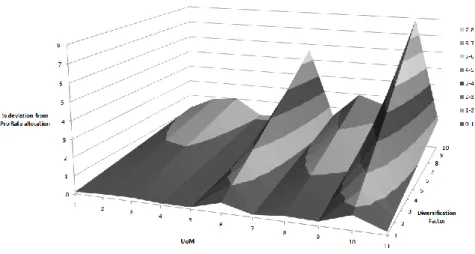
In this section we investigate the sensitivity of the calculated Shapley values to the diversification factor. If the mean is used to calculate the diversification factor instead of the median, a value d ~ 9.1% emerges. Hence we consider a range of diversification factors from 1 to 10, and recalculate the Shapley values using (10) for the constant diversification case and (12) for the diminishing diversification case. The results in Figures 4 and 5 respectively show deviations of the Shapley allocations from the corresponding Pro Rata allocations, expressed as percentages. The labels on the "UoM" axis correspond to the 11 UoMs P2, ..., P12. The service P1 is not shown. The main points of the charts are:
The profiles look very similar, the main difference being that the Shapley values are much higher for the constant diversification case.
Slicing parallel to the UoM axis results in similar profiles for all diversification factors As the diversification factor increases, the Shapley values in the constant diversification case
increase linearly, and the Shapley values in the diminishing diversification case increase almost linearly. In the latter case, the slight non-linearity due the rapid reduction of the factor dr for r > 2 is not apparent in Figure 4.
No ill-conditioning is apparent.
Figure 5: Sensitivity of Shapley allocations to diminishing diversification factor
It should be stressed that the method of calculating the diversification factor (section 5.1) is one of many. We are keen to explore whether or not it can be done (quickly and easily!) by considering a correlation structure.
6 Conclusion
We have proposed an allocation methodology that is applicable to a large number of operational risk UoMs, including a service in the form of a support function. Using the Shapley method, we can account for diversification by considering coalitions. For the intended number of UoMs (8-100), it is not feasible to do exact calculations for two reasons. First, the combinatorial complexity prevents it. Second, there is no standard way to calculate the value of a coalition. We therefore assume initially that all UoMs contribute to a coalition in the same way, so that they each add a value proportional to their stand-alone value when they enter a coalition. Refining this assumption, so that the added value on joining a coalition decreases as the size of the coalition increases, models the case where any new entrant to a large coalition adds minimal value. The effect of the service is to absorb allocation from all other UoMs.
There are three principal results of this analysis.
1. The allocations of all UoMs decrease relative to their Pro Rata allocations, which makes the result acceptable to risk managers.
2. We have derived closed-form expressions for Shapley allocations, which can be used for a large number of UoMs, and take negligible computation time.
3. We have modelled a service as an entity that moderates the capital of UoMs by absorbing capital from them.
Examination of the dependency structure of the UoMs using correlations and copulas reveals that there is no straightforward relationship between the diversification factor obtained by any one method and any other. The results for the dependency structure analyses produce a result which are of similar
orders, but differ in detail. In principle, we would like to use our allocation method as an alternative to formulating a formal dependency structure by considering correlations or a copula. In this context, its use would be to reduce overall regulatory capital by the amount of the diversification factor. This procedure now seems a reasonable way forward.
We have also assumed that no dominance exists. The concept of dominance is worthy of a much larger study, particularly if we measure dominance as a function of capital value.
Appendix A
Proof of Proposition 1
For n players P1, P2,…,Pn with values v1, v2,…,vn, define a cost function by
v(CU P) = v(C) + v(P) -dv(P) where 0 <d< 1 is a constant factor. Then the Shapley value of player Pr is given by
SH(n, r) = vr – (1 – 1/n)dvr
Proof
If there are n players, there are n! permutations of players. Consider permutation j. Let [r] be the position of Pr in permutation j. There are two cases to consider: r = 1 and 2 ≤ r ≤ n
When Pr is the first to enter a coalition, the marginal allocation for Pr is vr, and there are (n-1)! such
cases. Therefore there is a contribution to the sum of marginals for Pr:
M(Pr) = vr(n-1)! (A1)
When Pr is not the first to enter a coalition, let [k] be the position of Pr in permutation. The marginal
allocation for Pr is the difference between the values of the coalitions C = {P[1], P[2],…, P[k-1}} and {P[1],
P[2],…, P[k]}. Using the cost function of the proposition this is
M(1)(Pr) = v(CUP[k]) -v(C)
=v(P[k]) -dv(P[k])
= vr - dvr
The above difference applies for [n! - (n-1)!] cases. Therefore there is a further contribution to the sum of marginals for Pr:
M(2)(Pr) = (vr– dvr)×[n! - (n-1)!] (A2)
The Shapley value for Pr is therefore given by the mean of (A1) + (A2).
n!SH(n, r) = M(1)(Pr) + M(2)(Pr)
= vr(n-1)! + (vr– dvr)×[n! - (n-1)!]
Therefore
SH(n, r) = vr - (1- 1/n)dvr (A3)
Appendix B
Proof of Proposition 2
The Shapley values for the non-service players Pr (2 ≤ r ≤ n) and the Service P1 are given by
SH(n,r) = vr - - dvr(1 – 1/n) - dm(1n) (2 ≤ r ≤ n)
SH(n,1) = (n-1)+ (n-1)dm(1n)
The proof proceeds by enumerating cases for the n! permutations of the players. In each permutation, players enter a coalition in order, and we consider the case where P1enters separately from the others.
Another distinction is whether or not a player (service or not) is the first to enter the coalition. For n-1non-service players P2,…,Pn with values v2-…,vn- define a cost function by
v(CUPr) = v(C) + v(Pr) -dvr- dm= v(C) + vr- - dvr - dm where 0 <d< 1 is a constant factor and m is the
median of v2…,vn.
The Service player P1 has value (n-1), and define its cost function by
(CU P1) = v(C) + (n-1) + (n-1)dm a
Case 1: P1 is first in the permutation: allocation is to the service P1
P1 is first (n-1)! times out of n!, and the marginal allocation to P1 each time is (n-1). The total
marginal allocation for this case is
M(1)(P1) = (n-1)!×(n-1)
Case 2: P1 is not first in the permutation: allocation is to the service P1
P1 is not first [n! - (n-1)!] times. When P1 joins the coalition, P1 receives a marginal allocation
(n-1)(n-1)dmTherefore the total marginal allocation for this case is
M(2)(P1) = [n! - (n-1)!]×[(n-1)(n-1)dm
Case 3: Pr (a non-service) is first in the permutation: allocation is to Pr
Pr is first in (n-1)! cases, each with marginal allocation vr - . There is no diversification. The
total marginal allocation for this case is
M(3)(Pr) = (n-1)!×(vr - )
Case 4: Pr is not first in the permutation: allocation is to Pr
Pr is not first in [n! - (n-1)!] cases. Suppose that Pr enters the coalition at the k-th place, so
that r = [k]. Then the marginal allocation to Pr is the difference between the values of the
coalitions C = {P[1], P[2],…, P[k-1}} and {P[1], P[2],…, P[k]}. Using (B1) this is
M(3)(Pr) = v(CU P[k]) - v(C)
The total marginal allocation for this case is then
M(4)(Pr) = [n! - (n-1)!]×(vrdvr- dm) (B5)
By symmetry, all non-service players can be analysed in the same way and have the results that follow the same pattern.
The total marginal allocation for P1, M(P1) is the sum of the marginal in (B2) and (B3).
M(P1) = M(1)(P1) + M(2)(P1)
= (n-1)!×(n-1) + [n! - (n-1)!]×[(n-1)ndm
n!×(n-1)dnm[n! - (n-1)!] The total marginal allocation for Pr, M(Pr) is the sum of the marginal in (B4) and (B5).
M(Pr) = M(3)(Pr) + M(4)(Pr)
= (n-1)!×(vr - ) [n! - (n-1)!]×(vrdvr-dm)
= n!×(vrdvrdm) + d(vr + m)(n-1)! (B7)
The final stage in the proof is to calculate the mean marginal allocation by dividing (B6) and (B7) by the total number of permutations, n!
SH(n,1) (n-1) (n-1)dm(1n) SH(n,r) = vrdvr(1n)dm(1n) (2 ≤ r ≤ n)
This completes the proof of Proposition2, and Equation (B8) corresponds to (10).
Appendix C
Proof of Proposition 3
For n-1non-service players P2,…,Pn with values v2-…,vn-, define a cost function for when a new
non-service player Pr joins a coalition C as
(CUPr) = v(C) + v(Pr) - d|C|vr - d|C|m. (C1)
where m is the median of the values v2,…,vn and d is a diversification factor in (0, 1).
The Service player P1 has value (n-1), and define its cost function by
(CU P1) = v(C) + (n-1) + (n-1)d|C|m (C1a)
We therefore state Proposition 3:
The Shapley values for the non-service players Pr (2 ≤ r ≤ n) and the Service P1 under conditions of
diminishing diversification given in (C1 and C1a) are given by SH(n,r) = vr - - (m + vr)Dn/n (2 ≤ r ≤ n)
SH(n,1) = (n-1)+ (n-1)mDnn
where Dn = dd2 + ... +dn-1.
Proof:
The proof is similar to that of Appendix B, but the enumerations are different. There are the same four cases.
Case 1: P1 is first in the permutation: allocation is to the service P1
P1 is first (n-1)! times out of n!, and the marginal allocation to P1 each time is (n-1)(from
Equation 7). The total marginal allocation for this case is
M(1)(P1) = (n-1)!×(n-1) C
Case 2: P1 is not first in the permutation: allocation is to the service P1
P1 is not first [n! - (n-1)!] times. When P1 joins the coalition, P1 receives a marginal allocation
(n-1)Additionally there are (n-1)! diversification cases of each of the following, to be added:
(n-1)md, (n-1)md2, ..., (n-1)mdn-1.
Therefore the total marginal allocation for this case is
M(2)(P1) = [n! - (n-1)!]×(n-1)(n-1)! (n-1)mdd2 + ... +dn-1
Case 3: Pr (a non-service) is first in the permutation: allocation is to Pr
Pr is first in (n-1)! cases, each with marginal allocation vr - . There is no diversification. The
total marginal allocation for this case is
M(3)(Pr) = (n-1)!×(vr - ) C
Case 4: Pr is not first in the permutation: allocation is to Pr
Pr is not first in [n! - (n-1)!] cases. When Pr joins the coalition, Pr receives a marginal allocation
(vr - in all of those casesAdditionally there are (n-1)! diversification cases of each of the
following, to be subtracted: vrd, vrd2, ..., vrdn-1,
md, md2, ..., mdn-1.
The total marginal allocation for this case is then
M(4)(Pr) = [n! - (n-1)!]×(vr)(n-1)!(vr + mdd2 + ... +dn-1
[n! - (n-1)!]×(vr)(n-1)!(vr + mDn (C5)
By symmetry, all non-service players can be analysed in the same way and have the results that follow the same pattern.
The total marginal allocation for P1, M(P1) is the sum of the marginal in (C2) and (C3).
M(P1) = M(1)(P1) + M(2)(P1)
= (n-1)!×(n-1) +[n! - (n-1)!]×(n-1)(n-1)! (n-1)mDn
n!×(n-1) (n-1)m(n-1)!Dn C6
The total marginal allocation for Pr, M(Pr) is the sum of the marginal in (C4) and (C5).
M(Pr) = M(3)(Pr) + M(4)(Pr)
= (n-1)!×(vr - )[n! - (n-1)!]×(vr)(n-1)!(vr + mDn
= n!×(vr(vr -+m)Dn(n-1)! (C7)
The final stage in the proof is to calculate the mean marginal allocation by dividing (C6) and (C7) by the total number of permutations, n!
SH(n,1) (n-1) (n-1)mDnn
SH(n,r) = vr(vrm)Dnn (2 ≤ r ≤ n) C8
References
Aumann,R. and Shapley,L. Values of Non-Atomic Games. Princeton University Press (1974)
Butler,M. and Williams,H.P. The Allocation of Shared Fixed Costs. European Journal of Operational Research, 170 (2006)
BCBS196 The Basel Committee on Banking Supervision: "Supervisory Guidelines for the Advanced Measurement Approaches" (2011)
Castro,J., Gómez,D. and Tejada,J. Polynomial Calculation of the Shapley value based on Sampling. Computers and Operations Research, 36, 1726-1730, Elsevier (2009)
Dehez,P. Allocation of fixed costs: characterization of the (dual) weighted Shapley value. International Game Theory Review, 13(2), 141-157 (2011)
Frachot, A, Georges,P. and Roncalli, T. Loss Distribution Approach for Operational Risk SSRN: http://ssrn.com/abstract=1032523 orhttp://dx.doi.org/10.2139/ssrn.1032523 (2001)
Garcia-Diaz, A. and Lee, D-J. Models for Highway Cost Allocation, ch. 6 in “Game Theory Relaunched", ed. Hanappi,H. INTECH (2013)
Junqueira,M., da Costa,L., Barroso,L., Oliveira,G., Thomé,L. and Pereira,M. An Aumann-Shapley Approach to AllocateTransmission Service Cost Among Network Users in Electricity Markets. IEEE Transactions on Power Systems, 22(4) (2007)
Leippold,M. and Vanin,P. The Quantification of Operational Risk. SSRN:http://ssrn.com/abstract=481742 or http://dx.doi.org/10.2139/ssrn.481742 (2003)
Liben-Nowell,D., Sharp, A., Wexler, T. and Woods, K. Computing Shapley Value in Supermodular Coalitional Games. Computing and Combinatorics: Lecture Notes in Computer Science 7434, 568-579 (2012)
Linhart,P., Radner,R., Ramakrishnan,K. and Steinberg,R. The allocation of value for jointly provided services. Telecommunication Systems, 4,151-175 (1995)
Littlechild,S. and Owen,G. A simple Expression for the Shapley Value in a special case. Management Science, 20(3), Inst. of Management Science (1973)
Littlechild, S. and Thompson,G. Aircraft Landing Fees: A Game Theory Approach. The Bell Journal of Economics, 8(1) , 186-204, The RAND Corporation (1977)
Markowitz, H.M. Portfolio Selection. The Journal of Finance 7 (1), 77–91, (1952) Milliman Aggregation of risks and Allocation of capital. .Milliman Research Report,
http://www.milliman.com/uploadedFiles/insight/research/life-rr/aggregation-of-risks-allocation.pdf (2009)
Monti,F., Brunner,M., Piacenza,F. and Bazzarello,D. Diversification effects in operational risk: A robust approach. Journal of Risk Management in Financial Institutions, 3(3), 243-258. Henry Stewart (2010)
Peleg,B. Coalition formation in simple games with dominant players. International Journal of Game Theory 10(1) 11-33 (1981)
Press, W. H., Flannery, B. P., Teukolsky, S. A., and Vetterling, W. T. Cholesky Decomposition §2.9 (89-91), Numerical Recipes in FORTRAN: The Art of Scientific Computing. Cambridge University Press (1992) Shapley, L A value for n-person Games. The Rand Corporation, (1953). Also in The Shapley value: Essays in honor of Lloyd S. Shapley (ed. Roth,A.) CUP (1988)
Tarashev,N., Borio,C., and Tsatsaronis,K The systemic importance of financial institutions, in BIS Quarterly Review (page 77), Bank for International Settlements. (2009)
Wagner,W.H. and Lau,S. C. The Effect of Diversification on Risk, Financial Analysts Journal, 27(6), 48-53, CFA Institute (1971)