Production and transport of long lifetime excited states in pre-equilibrium ion solid collisions

HAL Id: hal-00021933

https://hal.archives-ouvertes.fr/hal-00021933

HAL is a multi-disciplinary open access archive for the deposit and dissemination of sci-entific research documents, whether they are pub-lished or not. The documents may come from teaching and research institutions in France or abroad, or from public or private research centers.

L’archive ouverte pluridisciplinaire HAL, est destinée au dépôt et à la diffusion de documents scientifiques de niveau recherche, publiés ou non, émanant des établissements d’enseignement et de recherche français ou étrangers, des laboratoires publics ou privés.

Production and transport of long lifetime excited states

in pre-equilibrium ion solid collisions

Emily Lamour, Benoit Gervais, Jean Pierre Rozet, Dominique Vernhet

To cite this version:

Emily Lamour, Benoit Gervais, Jean Pierre Rozet, Dominique Vernhet. Production and transport of long lifetime excited states in pre-equilibrium ion solid collisions. Physical Review A, American Physical Society, 2006, 73, pp.042715. �10.1103/PhysRevA.73.042715�. �hal-00021933�

TABLES

TABLE I. Respective contribution of direct and cascade population to the total population for different nl states and two target thickness. The direct contribution corresponds to the population at the exit of the foil. The cascade contribution corresponds to the population coming from upper levels by radiative decay behind the foil.

3.5 µg/cm2target 98 µg/cm2 target n_{l state} % direct % cascade % direct % cascade

2p 60 40 51 49

2s 74 26 84 16

3p 89 11 86 14

TABLE II. Energy of each observed line with the associated efficiency and global transmission for one of the Si(Li) detector. The efficiency of the other Si(Li) detector corresponds to 70% of the values given here. EProj and ELab correspond respectively

to energies in the projectile and laboratory frames. Energies of the Lyman line are taken from Ref[23]. "*" marks energy of the centre of the theoretical distribution of the 2E1 decay mode Ref [22].

Energy (eV) Si(Li) detector

Observed

Lines EProj ELab

(θL=90°) Efficiency nl glob T Lyα 3321 3273 0.83 (±7%) 8.62 10-6 (±9.5%) Lyβ 3936 3879 0.88 (±7%) 9.20 10-6 (±9.5%) Lyγ 4150 4091 0.90 (±7%) 9.36 10-6 (±9.5%)

∑

FIGURES CAPTIONS

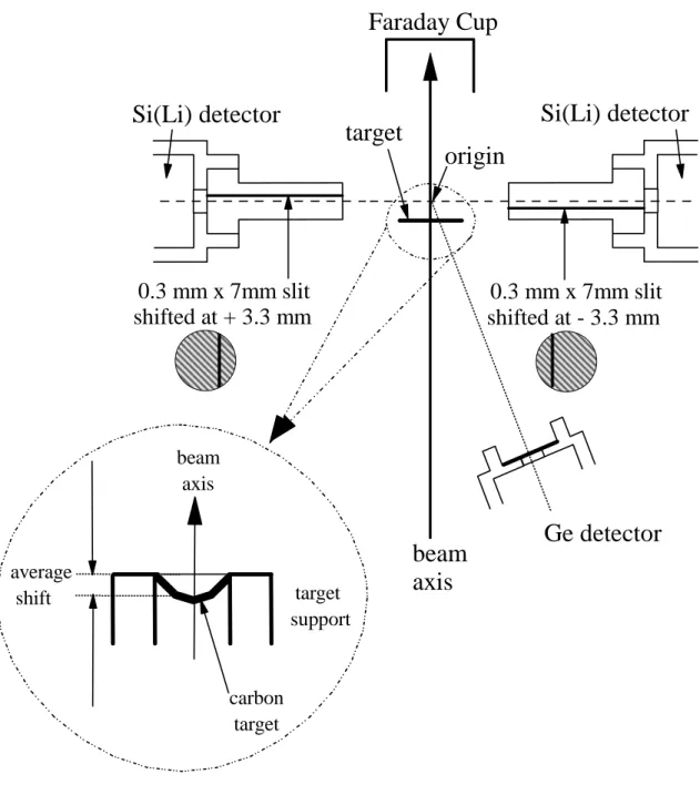
FIG. 1. Schematic representation of the experimental set-up. Effects leading to X-ray auto-absorption are displayed in a zoom (see text).

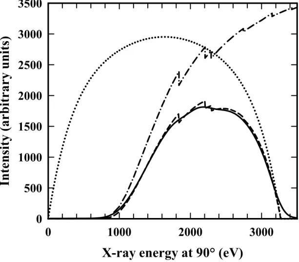
FIG. 2. Energy distribution of the 2E1 decay mode for an Ar17+ ion: the theoretical distribution (dotted line), the distribution corrected by the Si(Li) detector efficiency alone (dashed line) and the "experimental" distribution (solid line) i.e. the distribution corrected by the efficiency convoluted with the detector resolution. Si(Li) detector efficiency is also plotted (dash-dotted line) for sake of clarity.

FIG. 3. Spectra recorded by a Si(Li) detector after backgrounds subtraction at various ion time of flight (delay time) behind the 3.5 µg/cm2 carbon target: (a) t = 0; (b) t = 108 ps; (c) t = 600 ps.

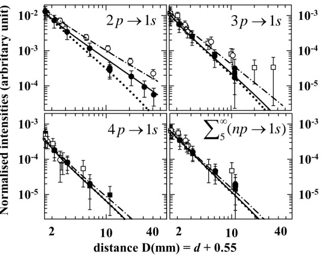
FIG. 4. Normalized evolution of the Lyman lines emission (see text) as a function of the distance behind the target: experimental data (symbols: ● target of 3.5 µg/cm2, ■ 8.6 µg/cm2_{, □ 98 µg/cm}2 _{and ○ 201 µg/cm}2_{), binary ion-atom conditions i.e. including}

cascade contribution without any transport effects accounted for (dotted curves), classical transport "wake off" (solid curves: target of 3.5 µg/cm2, dashed dotted curves: 201 µg/cm2). The real distance d behind the target has been arbitrary shifted by 0.55 mm to clarify the graph.

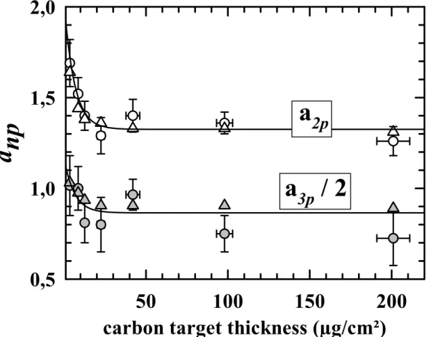
FIG. 5. Slope evolution of the delayed Lyman line intensities versus foil thickness; circles with error bars: experiment (symbols with error bars); classical transport (triangles); fit with a decay function given in the text (solid lines). The a3p has been

divided by 2 to clarify the graph.

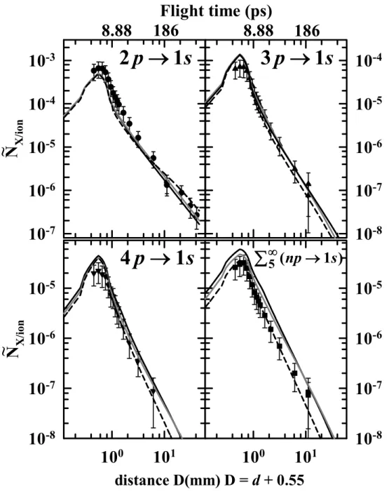
FIG. 6. Evolution with the time of flight of the Ar17+ Lyman line intensities (i.e. number of emitted photon per ion) for the 3.5 µg/cm2 carbon target: experimental results (symbols), classical transport model "wake off" (solid black lines) and "wake on" (solid grey lines), rate equation model (dashed lines). In the simulations, the CDW calculations have been used to account for the primary capture processes. The distance behind the target has been arbitrary shifted by 0.55 mm for sake of clarity.

FIG. 7. Same as Fig. 6 for the 8.6 µg/cm2 target thickness.

FIG. 8. Same as Fig. 6 for the 12.6 µg/cm2 target thickness.

FIG. 9. Same as Fig. 6 for the 42 µg/cm2 _{target thickness.}

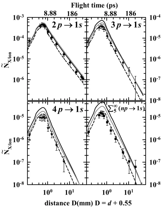
FIG. 10. Same as Fig. 6 for the 98 µg/cm2 target thickness.

FIG. 11. Absolute 2s1/2 populations of Ar17+ at vp = 23 a.u. impact velocity as a

conditions i.e. including cascade contribution without any transport effects accounted for (dotted black curve); classical transport model "wake off" (solid black line) and "wake on" (solid grey line); rate equations model (dashed black line); Master equations model with complete CDW calculations to describe the initial capture process (dashed grey line) and Master equations model with CDW calculations and with the phases of coherences of the initial states taken equal to zero (dash-dot-dotted grey line).

FIG. 12. Geometrical efficiency function of Si(Li) detectors for z ≥ 0.87; z is the position of the target support and Z the position where nl → 1s transitions are recorded.

FIG. 13. Geometrical efficiency function of Si(Li) detectors for 0.55 ≤ z ≤ 0.87; z is the position of the target support and Z the position where nl → 1s transitions are recorded. The hatched area is hidden by the support.

FIG. 14. Geometrical efficiency function of Si(Li) detectors for 0.25 + e ≤ z ≤ 0.55; z is the position of the target support and Z the position where nl → 1s transitions are recorded. The parameters e and δ(z) are defined in the text. The hatched area is hidden by the support.

FIG. 15. Geometrical efficiency function of Si(Li) detectors for - 0.07 + e' ≤ z≤ 0.25 +

are recorded. The parameters e, e' and δ(z) are defined in the text. The hatched area is hidden by the support.

FIG. 16. Geometrical efficiency function of Si(Li) detectors for 0.25 ≤ z ≤ 0.87; z is the position of the target support and Z the position where nl → 1s transitions are recorded. The hatched area is hidden by the support.

FIG. 1. Schematic representation of the experimental set-up. Effects leading to X-ray auto-absorption are displayed in a zoom (see text).

Si(Li) detector

Si(Li) detector

Ge detector

target

origin

0.3 mm x 7mm slit

shifted at + 3.3 mm

Faraday Cup

0.3 mm x 7mm slit

shifted at - 3.3 mm

beam

axis

FIG. 2. Energy distribution of the 2E1 decay mode for an Ar17+ ion: the theoretical distribution (dotted line), the distribution corrected by the Si(Li) detector efficiency alone (dashed line) and the "experimental" distribution (solid line) i.e. the distribution corrected by the efficiency convoluted with the detector resolution. Si(Li) detector efficiency is also plotted (dash-dotted line) for sake of clarity.

X-ray energy at 90° (eV)

0

1000

2000

3000

In

ten

sity

(a

rb

itra

ry

u

n

its)

0

500

1000

1500

2000

2500

3000

3500

FIG. 3. Spectra recorded by a Si(Li) detector after backgrounds subtraction at various ion time of flight (delay time) behind the 3.5 µg/cm2 carbon target: (a) t = 0; (b) t = 108 ps; (c) t = 600 ps.

10

10

10

10

N

orm

alized

in

te

n

sit

ies (

arb

it

rary u

n

it

)

10

10

10

10

Energy (eV) at 90°

1000

2000

3000

4000

10

10

10

Ly

α'

Ly

β

Ly

γ

Si-escape peak

Si-escape peak

2E1

Ly

α'=Lyα+M1

Ly

β

Ly

γ

2E1

Ly

α'=Lyα+M1

(a)

(b)

(c)

∑

∑

FIG. 4. Normalized evolution of the Lyman lines emission (see text) as a function of the distance behind the target: experimental data (symbols: ● target of 3.5 µg/cm2, ■ 8.6 µg/cm2, □ 98 µg/cm2 and ○ 201 µg/cm2), binary ion-atom conditions i.e. including cascade contribution without any transport effects accounted for (dotted curves), classical transport "wake off" (solid curves: target of 3.5 µg/cm2, dashed dotted curves: 201 µg/cm2). The real distance d behind the target has been arbitrary shifted by 0.55 mm to clarify the graph.

10

10

10

10

10

10

distance D(mm) = d + 0.55

10

10

10

10

N

orm

alis

ed

int

en

sit

ies

(

arbrit

ary u

n

it

)

10

10

10

10

∑

∞

→

5

(

np

1

s

)

s

p

1

2

→

3

p

→

1

s

s

p

1

4

→

2

40

2

40

FIG. 5. Slope evolution of the delayed Lyman line intensities versus foil thickness; circles with error bars: experiment (symbols with error bars); classical transport (triangles); fit with a decay function given in the text (solid lines). The a3p has been

divided by 2 to clarify the graph.

carbon target thickness (µg/cm²)

50

100

150

200

a np

0,5

1,0

1,5

2,0

a

_2p

a

_3p

/ 2

FIG. 6. Evolution with the time of flight of the Ar17+ Lyman line intensities (i.e. number of emitted photon per ion) for the 3.5 µg/cm2 carbon target: experimental results (symbols), classical transport model "wake off" (solid black lines) and "wake on" (solid grey lines), rate equation model (dashed lines). In the simulations, the CDW calculations have been used to account for the primary capture processes. The distance behind the target has been arbitrary shifted by 0.55 mm for sake of clarity.

N

10

10

10

10

10

10

10

10

10

10

10

₁₀

N

10

10

10

10

distance D(mm) D = d + 0.55

10

₁₀

10

10

10

10

8.88

186

8.88

186

Flight time (ps)

~

~

s

p

1

2

→

s

p

1

4

→

∑

(

np

→

1

s

)

s

p

1

3

→

FIG. 7. Same as Fig. 6 for the 8.6 µg/cm2 target thickness.

N

10

10

10

10

10

10

10

10

10

10

distance D(mm) D = d + 0.55

10

₁₀

N

10

10

10

10

10

10

₁₀

10

10

10

10

10

~

~

8.88 186

Flight time (ps)

8.88

186

s

p

1

2

→

s

p

1

4

→

∑

(

np

→

1

s

)

s

p

1

3

→

FIG. 8. Same as Fig. 6 for the 12.6 µg/cm2 target thickness.

10

10

10

10

10

10

₁₀

N

10

10

10

10

distance D(mm) D = d + 0.55

10

₁₀

10

10

10

10

8.88

186

8.88

186

Flight time (ps)

~

~ N

10

10

10

10

s

p

1

2

→

s

p

1

4

→

∑

∞

₅

(

np

→

1

s

)

s

p

1

3

→

FIG. 9. Same as Fig. 6 for the 42 µg/cm2 target thickness.

10

10

10

10

10

N

10

10

10

10

10

10

₁₀

N

10

10

10

10

10

distance D(mm) D = d + 0.55

10

₁₀

10

10

10

10

10

~

~

8.88

186

8.88

186

Flight time (ps)

s

p

1

2

→

s

p

1

4

→

∑

∞

₅

(

np

→

1

s

)

s

p

1

3

→

FIG. 10. Same as Fig. 6 for the 98 µg/cm2 target thickness.

N

10

10

10

10

10

10

10

10

10

10

10

10

10

₁₀

N

10

10

10

10

10

distance D(mm) D = d + 0.55

10

₁₀

10

10

10

10

10

8.88 186

Flight time (ps)

8.88 186

~

~

s

p

1

2

→

s

p

1

4

→

∑

∞

₅

(

np

→

1

s

)

s

p

1

3

→

FIG. 11. Absolute 2s1/2 populations of Ar17+ at vp = 23 a.u. impact velocity as a

function of carbon target thickness: experimental data (symbols); binary ion-atom conditions i.e. including cascade contribution without any transport effects accounted for (dotted black curve); classical transport model "wake off" (solid black line) and "wake on" (solid grey line); rate equations model (dashed black line); Master equations model with complete CDW calculations to describe the initial capture process (dashed grey line) and Master equations model with CDW calculations and with the phases of coherences of the initial states taken equal to zero (dash-dot-dotted grey line).

carbon target thickness (µg/cm²)

1

10

100

2s

1/

2

po

pula

tion/ion

10

-3

10

-2

FIG. 12. Geometrical efficiency function of Si(Li) detectors for z ≥ 0.87; z is the position of the target support and Z the position where nl → 1s transitions are recorded. Z ) (Z g ε beam axis z 0.3 mm 60.4 mm 124.8 mm 0.87 1 target support 0.55 0.25 -0.07

FIG. 13. Geometrical efficiency function of Si(Li) detectors for 0.55 ≤ z ≤ 0.87; z is the position of the target support and Z the position where nl → 1s transitions are recorded. The hatched area is hidden by the support.

Z ) (Z g ε beam axis z 0.3 m m 60.4 mm 124.8 mm 0.87 1 target support 0.55 0.25 -0.07

FIG. 14. Geometrical efficiency function of Si(Li) detectors for 0.25 + e ≤ z ≤ 0.55; z is the position of the target support and Z the position where nl → 1s transitions are recorded. The parameters e and δ(z) are defined in the text. The hatched area is hidden by the support.

Z ) (Z g ε beam axis z 0.3 m m 60.4 mm 124.8 mm 0.87 1 target support 0.55 0.25 -0.07 δ (z)

FIG. 15. Geometrical efficiency function of Si(Li) detectors for - 0.07 + e' ≤ z≤ 0.25 +

e; z is the position of the target support and Z the position where nl → 1s transitions

are recorded. The parameters e, e' and δ(z) are defined in the text. The hatched area is hidden by the support.

Z ) (Z g ε beam axis z 0.3 m m 60.4 mm 124.8 mm 0.87 1 target support 0.55 0.25 -0.07 δ (z)

FIG. 16. Geometrical efficiency function of Si(Li) detectors for 0.25 ≤ z ≤ 0.87; z is

the position of the target support and Z the position where nl → 1s transitions are

recorded. The hatched area is hidden by the support. Z ) (Z g ε beam axis z 0.3 m m 60.4 mm 124.8 mm 0.87 1 target support 0.55 0.25 -0.07 target support