Price Stability and the ECB'S monetary policy strategy

HAL Id: hal-00308557

https://hal.archives-ouvertes.fr/hal-00308557

Submitted on 31 Jul 2008

HAL is a multi-disciplinary open access

archive for the deposit and dissemination of sci-entific research documents, whether they are pub-lished or not. The documents may come from teaching and research institutions in France or abroad, or from public or private research centers.

L’archive ouverte pluridisciplinaire HAL, est destinée au dépôt et à la diffusion de documents scientifiques de niveau recherche, publiés ou non, émanant des établissements d’enseignement et de recherche français ou étrangers, des laboratoires publics ou privés.

Price Stability and the ECB’S monetary policy strategy

Christian Bordes, Laurent Clerc

To cite this version:

Christian Bordes, Laurent Clerc. Price Stability and the ECB’S monetary policy strategy. Journal of Economic Surveys, Wiley, 2007, 21 (2), pp.268 - 326. �10.1111/j.1467-6419.2006.00504.x�. �hal-00308557�

NOTES D’ÉTUDES

ET DE RECHERCHE

PRICE STABILITY AND THE ECB’S

MONETARY POLICY STRATEGY

Christian Bordes and Laurent Clerc

March 2004

DIRECTION GÉNÉRALE DES ÉTUDES ET DES RELATIONS INTERNATIONALES

DIRECTION DES ÉTUDES ÉCONOMIQUES ET DE LA RECHERCHE

PRICE STABILITY AND THE ECB’S

MONETARY POLICY STRATEGY

Christian Bordes and Laurent Clerc

March 2004

NER # 109

Les Notes d'Études et de Recherche reflètent les idées personnelles de leurs auteurs et n'expriment pas nécessairement la position de la Banque de France. Ce document est disponible sur le site internet de la Banque de France «www.banque-France.fr».

The Working Paper Series reflect the opinions of the authors and do not necessarily express the views of the Banque de France. This document is available on the Banque de France Website “www.banque-France.fr”.

Price stability and the ECB’s monetary policy strategy

Christian Bordes

1

_{and Laurent Clerc}

2

March 2004

1_{University of PARIS 1 – Panthéon - Sorbonne. E-mail :christian.bordes@univ-paris1.fr} 2_{Banque de France. E-mail :laurent.clerc2@banque-france.fr}

The views expressed in this paper are those of the authors and not necessarily those of either the University of Paris 1 or the Banque de France. We thank the participants of the Banque de France research seminar for useful discussions and particularly our discussant Massimo Rostagno (ECB). Any remaining errors are our sole responsibility.

Abstract:

This paper focuses on the price stability objective within the framework of the single monetary policy strategy. It starts by reviewing what this objective, which is common to all central banks, means. Secondly, this paper will focus exclusively on the anchoring of short- to medium-term inflation expectations (Part 2). Several measures show that this anchoring is effective. Modern New Keynesian theory is an appropriate framework for analysing the impact that this anchoring of expectations has on the determination of the short- to medium-term inflation rate. From this point of view, observed inflation in the euro area seems to be in line with the theory and the ECB’s action seems to be very effective. Thirdly, we will focus on the other aspect of monetary stability: the degree of price-level uncertainty and the anchoring of inflation expectations in the medium to long term. Even though this assessment is more difficult than it is in the short to medium term, since we only have a track record covering five years, various indicators from the theoretical analysis paint a fairly reassuring picture of the effectiveness of the device used by the ECB.

JEL Classification Number: E52, E58, E31

Non technical summary

I

- Price stability needs to be examined using two criteria: a) the stability of short- to medium-term inflation expectations; b) the absence of long-term price-level uncertainty. In practice, unfortunately, assessments of monetary strategies are all too frequently limited to the first criteria. - An inflation-targeting strategy is incomplete. It may ensure stability of the short- to medium-term

inflation rate, but it cannot guarantee monetary stability in the long term. Therefore, another device is needed to supplement it.

- Central banks that have adopted an inflation-targeting strategy have not specified the exact nature of the other device, even though some of them have mentioned it. On the other hand, in the case of the ECB’s strategy, which could be qualified as a “mixed” or “hybrid” strategy, the reference value for money growth should make it possible to regulate the price level in the long term.

II

- Since the single monetary policy was first applied, the short-term inflation dynamics has been disrupted by a series of temporary price shocks, but these shocks have not affected the anchor for inflation expectations, which have remained remarkably stable in a range between 1.5% and 2%. - The “New Keynesian” analytical framework is appropriate for the short to medium term: a policy

to anchor inflation expectations is an effective instrument for ensuring monetary stability. Furthermore, money can provide helpful information about future economic activity and, to a lesser extent, about price developments.

- Short- to medium-term inflation in the euro area has been in keeping with the main tenets of economic theory. A rough empirical review shows that: 1) There seems to be strong persistence of inflation, which nevertheless seems to have abated substantially since the implementation of the single monetary policy. 2) The change in the monetary regime did not give rise to greater uncertainty about the short-term inflation dynamics, except for a fleeting moment during the cash changeover to the euro. 3) The ECB’s monetary policy decisions seem to show that it has been less aggressive than New Keynesian theory would recommend (Taylor principle). However, the ECB’s response could be explained by the special attention paid to long-term inflation expectations.

III

- The highlights of an empirical analysis of the medium- to long-term inflation dynamics in the euro area are as follows: 1) The average annual steady-state inflation rate would be about 1.9%, which is “close to, but less than 2%”. The reversion to the steady state after a transient inflation shock is still quite slow. Reversion takes about seven years, because of the strong inertia of inflation. 2) The various measurements of long-term inflation expectations are consistent and stable in a range between 1.5% and 2%. The stability of these long-term expectations meant that the ECB did not have to act very aggressively.

- New Keynesian analysis on its own cannot provide a satisfactory explanation of the anchoring of long-term inflation expectations. Money plays a decisive role in the long term. From this point of view, the ECB’s announcement of a reference value for money growth is grounded on a sound theoretical basis.

- Yet it is difficult to assess the medium- to long-term effectiveness of the ECB’s monetary policy strategy after only four years of operation. However, a preliminary empirical analysis reveals some fairly reassuring signs. 1) A shock that affects short-term inflation expectations usually does

not have a knock-on effect on longer-term inflation expectations. 2) Since 1999, analysis has not rejected the hypothesis of price stationarity around a deterministic trend, which is a sign of long-term stability in the inflation rate and an absence of price-level uncertainty.

IV

- In terms of monetary policy strategy, the clarification provided at the end of the ECB Governing Council meeting on 8 May 2003 was useful in three respects in light of the conclusions of this report.

- The distinction drawn between “economic analysis”, which refers to the New Keynesian analytical framework, and “monetary analysis” is a relevant one, because it makes it possible to anchor short-, medium- and long-term inflation expectations simultaneously.

- It solves a problem in communicating and even implementing the single monetary policy strategy. This strategy was based on a presentation of the two “pillars” as alternative explanations for inflation, which could end up giving money a role in stabilising short-term anticipations that it would be unable to play. In fact, the two approaches are complements to each other rather than alternatives. Money plays a decisive role in anchoring long-term inflationary expectations, while the New Keynesian framework is adequate for analysing short-term expectations. This means that the change in the structure of the ECB President’s introductory statement following each Governing Council meeting will fully reflect the complementary nature of the two analytical frameworks.

- Finally, the anchoring of inflation expectations stemming from the announcement of the reference value and from the European Central Bank’s credibility ensures that there is no long-term price-level uncertainty. This means that monetary policy does not necessarily have to compensate for a deviation from the inflation path in the short term, since the reversion to the equilibrium path should be achieved via expectations.

Introduction

This paper focuses on the price stability objective within the framework of the single monetary policy strategy. It starts by reviewing what this objective, which is common to all central banks, means (Part 1). It encompasses two very distinct characteristics (Ireland, 1993): a) the anchoring of short- to medium-term inflation expectations; b) the absence of long-term price-level uncertainty. The ECB’s monetary strategy is aimed at achieving both objectives simultaneously in the euro-area economy. Secondly, this report will focus exclusively on the anchoring of short- to medium-term inflation expectations (Part 2). Several measures show that this anchoring is effective. Modern New Keynesian theory is an appropriate framework for analysing the impact that this anchoring of expectations has on the determination of the short- to medium-term inflation rate. From this point of view, observed inflation in the euro area seems to be in line with the theory and the ECB’s action seems to be very effective. The third part of this report will focus on the other aspect of monetary stability: the degree of price-level uncertainty and the anchoring of inflation expectations in the medium to long term (Part 3). The approach used in Part 2 of the report is used again in Part 3. We start with an empirical analysis aimed at revealing the steady-state inflation rate. This analysis reviews the various measures of expected long-term inflation in the euro area. The theoretical framework used in Part 2 is then supplemented by highlighting the role played by the announcement of a reference value for the growth of the money supply, which is intended to anchor long-term inflation expectations. This framework is then used to assess the effectiveness of the ECB’s action to ensure monetary stability in the long term. Even though this assessment is more difficult than it is in the short to medium term, since we only have a track record covering five years, various indicators from the theoretical analysis paint a fairly reassuring picture of the effectiveness of the device used.

As we can see, the analysis of monetary stability in the euro area hinges on the distinction between short- to medium-term developments on one side and the long-term prospects on the other. For the analysis to be complete, we need to look at each of these two aspects in turn, even though most of the available research all too frequently focuses exclusively on the first. What does this distinction mean in practice? The ECB mentions it explicitly when announcing its determination to control medium-term inflation in the euro area. Some observers have expressed regret that the ECB does not provide an operational definition of the medium term, but, at the same time, they state that it is by no means certain that such a definition could be provided (Gali, 2003). This point of view is probably excessive. A clear definition emerges from the research on the subject. Based on empirical studies of the relationships between money, economic activity and prices, we can agree on the following definitions (Issing et al, 2000; Jaeger, 2002): The short term is a period from one and a half to two years, during which money mainly influences economic activity. The medium term corresponds to a complete business cycle, lasting around five years. The long term is a period of eight to ten years, at least, during which the neutrality of money manifests itself, since variations in the money supply affect only the price level.

1. Monetary stability and the ECB’s strategy

1.1. What is monetary stability?

Strictly speaking, price stability is defined by two conditions: a) an absence of long-term price-level uncertainty; and b) an expected inflation rate of zero (Ireland 1993). The definition used in practice is often less strict. The second condition is not that stringent. Problems involved in measuring price increases accurately mean that a slightly positive expected inflation rate is deemed to satisfy this condition, as long as it is more or less constant. Some observers go even further and settle for fulfilment of the second condition and ignore the first condition. Price stability is therefore defined as a situation where “expected changes in the average price level are small enough and gradual enough that they do not materially enter business and household financial decisions” (Greenspan, 1989).

The pure and amended forms of the second condition are justified by the institutional approach that stresses the vulnerability of central banks in democratic societies. This approach was initially proposed by Kydland and Prescott (1977) and later developed by Barro and Gordon (1983). It is now expressed in the form of the expectations trap hypothesis to explain inflation dynamics (Christiano and Gust 2000; Christiano and Fitzgerald, 2003). If economic agents expect a high inflation rate, they take protective actions and the monetary authorities are faced with the following dilemma (Chart 1).

- They can validate the expectations by increasing money growth, which allows them to avoid a recession, but at the cost of higher inflation.

- They can abstain from increasing money growth, thus avoiding higher inflation, but inducing recession.

If the central bank is to avoid this trap and ensure monetary stability, it must make it clear that the first scenario must be ruled out. This is much easier to do if the central bank is independent from the government. But regardless of the central bank’s status, everything depends on its strategy. Prompt and decisive action in response to a substantial change in price-level expectations, meaning both inflation and deflation expectations, prevents the triggering of chain reactions that can quickly spin out of control. This calls for constant monitoring of the available indicators. The effectiveness of the authorities’ action can be assessed by examining developments in the expected inflation rate, as measured by surveys or indicators constructed from financial market data. As the observed inflation rate is equal to the expected inflation rate in the medium to long term, the first condition is deemed to hold when the (log) price level is stationary around a trend line.

Chart 1

Monetary policy strategy and anchoring expectations

Source: Christiano and Fitzgerald (2003) p. 24.

The first condition indicates that long-term price-level developments should be as steady as possible.3

There are many advantages to long-term price stability. It eliminates arbitrary wealth transfers, it reduces calculation and menu costs, it enhances the role that prices play in the allocation of resources and it eliminates the distortions of a tax system that applies to nominal values (see, for example, Barnett and Engineer, 1999).“With long-term inflation expectations more firmly anchored, long-term interest rates might jump around a bit less, and businesses and investors might find it easier to draw up long-term contracts” (Rogoff, 2003). Any uncertainty in this area makes decision-making more

3_{At this point, the definition of the long term is still fairly vague. It ranges from at least ten years to an average of twenty years. This}

difficult. Money does not fulfil its role of unit of account as well as it should and this penalises economic agents, including households saving for retirement and businesses that have to borrow short-term funds, since risk premiums make long-short-term financing more expensive. Consequently, deviations from the trend line, corresponding to the anchoring of expectations on a given value, must not be too large, otherwise uncertainty in the economic climate will increase and hamper investment and growth. As we have already mentioned, this characteristic of monetary stability is often overlooked. At first glance, this may seem only right; if inflation expectations are always anchored and, if there are no shocks to the economy, then there is no price-level uncertainty. Naturally, the real world is different. Central banks cannot control prices so strictly, nor do they want to, because, if they did and a shock occurred, they would have to accept major fluctuations in economic activity. This means that inflation may be higher or lower than expected over periods of varying lengths. If we consider that such deviations become permanent, meaning that the central bank does not attempt to correct past deviations, then long-term price-level developments become uncertain, despite the stability of inflation expectations. Consequently, we need to assess the success of a monetary stability strategy using the two criteria described at the outset.

1.2. Monetary stability programmes: the options available

The usual form of inflation target can be used to anchor expectations, but it does not ensure monetary stability in the full meaning of the term. This requires a supplementary device aimed at reducing long-term price-level uncertainty. On the other hand, a “Friedman” monetary rule would limit such uncertainty, but it could not ensure sufficiently solid anchoring of short-term expectations. In theory, the simplest solution to this problem is to set a price-level target. But this would entail other problems, which we shall discuss later. In practice, the solution is to adopt a mixed, or hybrid, strategy, where anchoring of expectations is backed up by a device that acts to force the price level back toward a regular trend (McCallum, 1997; Batini and Yates, 2001; Mishkin, 2000). Periodic review of the inflation target, or else the use of a reference value for money growth, can be considered as means towards this end.4

1.2.1. Incomplete strategies: inflation targets or money growth rules

Many central banks have opted for an inflation target. They adjust the interest rate according to expected developments in inflation at a time horizon that is generally between eighteen months and two years ahead. This strategy is an effective way of anchoring inflation expectations over the period concerned. But it may also entail a great deal of long-term price-level uncertainty (see Goodfriend, 1987). Inflation may in fact be higher or lower than expected. If we consider that deviations from the constant path are permanent, as is usually the case, the trend in the price level may be irregular in the long term, even though there is solid anchoring of inflation expectations in the shorter term. Everything depends on whether this volatility creates troublesome uncertainty that could disrupt the functioning of the economy. Some observers think that this is not the case. They use the following arguments (McCallum, 1997, pp. 18-19): a) few economic decisions are based on planning horizons over twenty years ahead; b) price-level uncertainty twenty years in the future is not large, even if the log price level behaves as a random walk. A confidence interval at the usual level of 95% would be only (plus or minus) 8% for the log price level at this horizon. This corresponds to a very low level of uncertainty compared to that observed in the nineteen-sixties through the nineteen-eighties. But, even if we accept this argument, which not all analysts do, the hybrid strategy is still better, because it provides the advantages of stationarity of the price level around a trend (McCallum, 1997, p. 19). Friedman (1960) proposed a constant-rate money supply growth rule. This rule should make a regular long-term trend in the price level possible if the relationship between money supply and prices is

4_{The list of hybrid strategies is longer. Mishkin (2000) suggests two others: 1) announcing an inflation target with a commitment to some}

error correction in which target misses will be offset to some extent in the future; 2) pursuing an inflation target under normal conditions, but providing for an escape clause that puts in place a price-level target in the event that deflation threatens, particularly if interest rates are near 0%.

stable over the period. To achieve this, the velocity of circulation and the economic growth rate must not be affected by permanent shocks. Even if we assume that this is the case, the relationship between money and prices cannot hold over a shorter period. This means that this strategy may have difficulty providing a solid anchor for expectations at all times. It is also in contradiction to the real-world situation, where central banks’ actions are taken in a short-term perspective and are aimed at controlling interest rates rather than the growth of a monetary aggregate.

1.2.2. Price-level targeting

A central bank may choose to announce a growth path for the price level, which is the same as setting a target for the average long-term inflation rate. The bank then attempts to correct deviations of the observed growth path from the preset growth path. The success of this strategy can be measured by the stationarity of the log price-level series around a linear trend. In this case, both characteristics of monetary stability can hold at the same time. One of the main advantages of this strategy would be to shelter the economy from the threat of deflation by curbing any price drift. If prices do fall, inflation expectations will automatically be revised upwards (Svensson, 1999). On the other hand, output and inflation would be more volatile than they would under an inflation-targeting regime. The reason for this is simple: when a shock pushes inflation up over its average trend, the inflation rate has to fall below the average later on. If the economy has nominal rigidities, the greater variability of the inflation rate would give rise to greater variability in output. However, this idea has been called into question by recent research showing that, under certain conditions relating to the formation of expectations and the persistence of output, this strategy can ensure greater long-term price stability without increasing the volatility of output (see Barnett and Engineer, 1999).

1.2.3. Combination of an inflation target and a price level target

King (1996) proposes a mixed strategy, with an inflation target for one and a half to two years ahead, along with periodic assessments every five years of the price level and a calculation of the average inflation rate for the period under review. In practice, this is the same as adopting an interest-rate rule to correct deviations of the observed inflation rate from the target for short- to medium-term inflation, as well as correcting the deviations of the observed variations from the desired price level. The price-level correction occurs at a more distant horizon of ten or more years ahead. In this case, interest rates are set according to the following rule:

÷÷ø

ö

ççè

æ

− + − + − + = * 1( *) 2( *) 3 _* * t t t t t t P P P y y i i

λ

λ

π

π

λ

where: λ3=λ2/Η and H denote the time horizon; yt-y* is the output gap; πt - π∗ is the deviation of observed inflation from the inflation target; Pt – P* is the deviation of the observed price level from the desired price level.5

1.2.4. Anchoring inflation expectations and the reference value for money growth.

Hetzel (1987, 1993) proposes some amendments to the strategy advocated by Friedman. Hetzel’s proposal, like Friedman’s, is based on the quantity theory of money and the principle of his proposal is derived from the same theory. But Hetzel amends and completes the theory on the basis of the observation that, in modern economies, the central bank does not have direct control over the quantity of money. Instead it controls the interest rate. According to the quantity theory of money, the central bank has to keep the interest rate at its equilibrium value in order to ensure price-level stability. This means that the central bank: a) adjusts its interest rate according to variations in the real interest rates; b) sets the interest rate so that the private sector can predict the future price level. In practice, the monetary authorities adjust the interest rate according to the deviation of the price-level path expected

by the private sector from the desired path, as measured, for example, via information provided by the index-linked bond market. At the same time, the authorities monitor money supply growth. The main difference with the previous strategy is that, if variations in money supply growth precede price-level changes, then the variable should be forced back toward the preset long-term path sooner. The ECB has chosen this type of strategy.

1.3. The ECB’s strategy

1.3.1. Hybrid strategy to ensure monetary stability

The monetary policy strategy of the ECB is price-stability oriented. The ultimate objective is defined in the Maastricht Treaty, where Article 105 (1) stipulates, “The primary objective of the ESCB shall be to maintain price stability. Without prejudice to the objective of price stability, the ESCB shall support the general economic policies in the Community with a view to contributing to the achievement of the objectives of the Community as laid down in Article 2.6 _{The ESCB shall act in}

accordance with the principle of an open market economy with free competition, favouring an efficient allocation of resources, and in compliance with the principles set out in Article 4.”7

After its meeting of 13 October 1998,8_{the Governing Council of the ECB described the main elements}

of its monetary policy strategy. From the outset, this strategy has hinged on: a) a quantitative definition of the price stability objective assigned to the ECB by the Maastricht Treaty, “a year-on-year increase in the Harmonised Index of Consumer Prices (HICP) for the euro area of below 2%”; b) an analysis that assigns a “prominent role for money” signalled by the announcement of a reference value,9 _{and based on “a broadly-based assessment of the outlook for price developments […] using a}

wide range of economic and financial variables”. The editorial in the first issue of the ECB Monthly Bulletin in January 1999 made this “two pillar” approach official.

Furthermore, the Governing Council’s definition stipulates that: a) price stability needs to be maintained in the medium term, thus acknowledging that there is short-term price volatility that cannot be controlled by monetary policy; b) the emphasis is placed on the HICP “for the euro area”, since monetary decisions are made according to developments relating to the euro area as a whole and not to specific regions or countries; c) the 2% threshold is the same as that previously targeted by most of the central banks in the euro area. With respect to the last point and in response to criticisms of the asymmetrical character of the definition, the ECB later explained that the expression “year-on-year increase in prices” automatically ruled out situations where prices fall (i.e. deflation).

Even though it really has not been called into question, except for some critics who would like to replace it with core inflation, the appropriateness of the choice of the HICP as the reference indicator for the quantitative definition of price stability was upheld during the internal evaluation exercise carried out in the Eurosystem (Camba-Mendez, 2003). The HICP has many advantages, such as its availability. It is one of the only harmonised indices calculated for the euro area as a whole. This automatically ensures comparability of prices across the European Monetary Union. The HICP also enjoys full credibility as a recognised and accepted measurement of price-level changes and it is available on a monthly basis. However, the HICP also has some shortcomings. It could be improved through more frequent revisions of the weights used at national level. In fact, only five out of the

6 _{Article 2 stipulates that “The Community shall have as its task […] to promote throughout the Community a harmonious, balanced and}

sustainable development of economic activities, a high level of employment and of social protection, […] sustainable and non-inflationary growth, a high degree of competitiveness and convergence of economic performance, a high level of protection and improvement of the quality of the environment”.

7_{In particular, Article 4 stipulates that the activities of the Member States and the Community shall include “the definition and conduct of a}

single monetary policy and exchange-rate policy the primary objective of both of which shall be to maintain price stability and, without prejudice to this objective, to support the general economic policies in the Community, in accordance with the principle of an open market economy with free competition.”

8_{See the Press Release dated 13 October 1998: “A stability-oriented monetary policy strategy for the ESCB”.} 9_{See the Press Release dated 1 December 1998: “The quantitative reference value for monetary growth”.}

twelve countries revise their weights on an annual basis. Furthermore, it is impossible to measure the margin of error in the measurement of prices in the euro area accurately.

In their reports to the French Council of Economic Analysis, Artus and Wyplosz (2002) state that the ECB’s inflation target of 2% is too low and that the implicit target range is too narrow. They recommend adopting range of 1% to 4% instead. Paul De Grauwe (quoted in an article in Le Monde, 29 January 2003, “La banque centrale européenne s’interroge sur son rôle”) suggests a smaller range of 2% to 3%. In a series of papers, Svensson (2002; 2003) maintains that the Eurosystem’s definition of price stability is ambiguous and asymmetrical and that it is less effective for anchoring expectations than a point target would be. He argues that an explicit and symmetrical point inflation target of 1.5%, 2% or 2.5% would be better and would provide a better anchor for inflation expectations. He also argues that, as long as a target value is announced clearly, it does not matter whether there is a range or not (Svensson, 2002).

But the most important thing is that the ECB’s strategy focuses on both aspects of monetary stability. This means that it can be regarded as a hybrid strategy aimed at anchoring medium-term inflation expectations, while simultaneously seeking to reduce long-term price-level uncertainty. As Jaeger (2002) so rightly stated, it can be seen as “a modified version of an inflation target, where the central bank avoids announcing a precise value or range for the medium-term inflation rate, while using an explicit nominal anchor (the reference value for M3 growth) to shape long-term inflation expectations”.

1.3.1. Real determinants of inflation and anchoring short- to medium-term expectations

In the short to medium term, the ECB’s monetary strategy stresses the role of the real determinants of inflation. This strategy is based on the widely accepted idea that monetary policy influences inflation in the following manner: changes in key interest rates influence short-term interest rates, short-term expectations with regard to economic activity and, through them, price-level changes. If follows that “a broadly based assessment of the outlook for prices and the risks to price stability in the euro area will play a major role in the Eurosystem’s strategy” (ECB, 1999a, p. 49). The appropriateness of monetary policy shall be assessed by considering inflation forecasts derived from wages, exchange rates, bond prices and the yield curve, various measures of real activity, price and cost indices and surveys of businesses and consumers.

1.3.3. Monetary determinants of inflation and anchoring medium- to long-term expectations

The ECB’s monetary strategy is also intended to anchor medium- to long-term expectations. “The statement that ‘price stability is to be maintained over the medium term’ reflects the need for monetary policy to have a forward-looking, medium-term orientation” (ECB, 1999a, p. 47, the emphasis is ours). The choice of method is based on the idea that monetary policy transmission mechanisms via the real sector are not the only channels through which the central bank influences prices. “There is broad consensus, based on substantial empirical evidence, that the development of the price level is a monetary phenomenon in the medium to long term” (ECB, 1999b, p. 29, the emphasis is ours). Over this period, “money constitutes a natural, firm and reliable ‘nominal anchor’ for monetary policy aiming at the maintenance of price stability” (ECB, 1999a, p. 47, the emphasis is ours). This means that money is given an important role through the announcement of a reference value for the growth of a monetary aggregate. “However, the concept of a reference value does not entail a commitment on the part of the Eurosystem to correct deviations of money growth from the reference value over the short term” (ibid. p. 48).

The ECB’s ability to anchor long-term inflation expectations has been the subject of much controversy. The critics are particularly severe with the core of the ECB’s monetary policy strategy. They generally advocate an alternative inflation-targeting strategy in its place. In a review of the practices and results of fifteen OECD countries’ central banks, Castelnuovo et al. (2003) show that most of these central banks, with the notable exception of Japan, have managed increasingly to anchor

agents’ long-term inflation expectations.10 _{This finding does not seem to depend on the strategic}

framework or on the way the inflation target is specified (i.e. as a point target or a range). To a certain extent, this research confirms the conclusions of Ball and Sheridan (2003), who cast doubt on the superiority of inflation-targeting strategies when it comes to stabilising prices, output and interest rates.

But, at what level should these inflation expectations be stabilised? The literature on finding the optimal inflation rate has basically split into two camps, between those that think that inflation acts like sand in the gears, slowing the economy down, and those who believe that it acts like grease. Generally speaking, empirical research shows that there is a negative relationship between growth and inflation, but that this relationship holds at relatively high levels of inflation. On the other hand, a recent paper by Rodriguez-Palenzuela et al (2003) shows that, in the case of the euro area, moderate levels of inflation would also produce “sand effects”. Yet, the euro area seems to be characterised by major nominal rigidities, which hints that even a low rate of inflation could promote flexibility in real wages and thus contribute to adjustment in the labour and goods markets, and ultimately boost growth. However, Coenen (2003b) uses a small macroeconomic structural model calibrated to fit the euro area to show that the impact of these nominal rigidities is small and that it is probably not significant for inflation rates over 1%.

However, the choice of an excessively low inflation target entails the risk of being confronted with the zero lower bound on nominal interest rates in the event of a major exogenous shock to the economy. Low inflation and its corollary, low nominal interest rates, limit the potential of the central banks’ main instrument. The banks cannot lower their official rates far enough, which means that real rates cannot fall enough to offset the effects of an unfavourable shock on the economy. Furthermore, when nominal interest rates are near zero, a deflationary shock could lead to a rise in real interest rates, which would be harmful for the economy. Simulations conducted using models calibrated to fit the euro area tend to show that the likelihood of running up against the zero constraint on nominal interest rates becomes negligible with an inflation target of 1% or more (Klaeffling and Perez, 2003). However, these results depend heavily on assumptions about the wage-setting procedures. More specifically, when wages are set in accordance with Taylor’s model11 _{(1979), the probability of}

running up against the zero constraint is less than 7%, if the inflation target is between 1% and 2%. On the other hand, the probability is no longer negligible when wage contracts are fixed in accordance with the model proposed by Fuhrer and Moore12 _{(1995). When the inflation target is zero, the}

probability is about 30%. It stands at 25% for a target of 1% and 17% for a target of 2% (Coenen, 2003a). Under the specifications for the second model, the existence of inflation rigidities, in addition to price rigidities, means that a fall in inflation entails a drop in activity, whereas, in the first model, lower inflation has no effect on output.

On 8 May 2003, the ECB presented the conclusions of an evaluation of its strategy. The evaluation was motivated by a determination to review its performance after four years of operation. The evaluation was intended as a response to the questions and comments of outside observers and it takes into account the findings of research by ECB staff. With regard to the price stability objective, which is the only one that interests us here, the Governing Council discussed the matter and decided to uphold the 2% upper bound for the inflation rate, as measured by the HICP. It also stated its “aim to maintain inflation rates close to, but below, 2% in the medium term”. It considered the costs of inflation and the need to maintain a sufficient safety margin to guard against the risks of deflation. It also addressed the issue of the possible measurement bias in the HICP and the implications of inflation differentials within the euro area.

10_{The long-term inflation expectations (10 years) are taken from the Consensus Forecast.}

11_{In this model, wages are set over the two periods and prices are determined by a constant mark-up on wages. This model induces price}

rigidity but not inflation rigidity.

2. Anchoring short- to medium-term expectations and inflation dynamics

What influence has the ECB’s monetary policy had on the euro area inflation rate in the short to medium term? We cannot answer this question without reference to an analytical framework. We shall present this framework after reviewing historical and expected inflation developments since 1999. The framework is then used to interpret these developments, with an effort to reveal the ECB’s contribution to price stability and its influence on inflation dynamics.

2.1. Short-term inflation and inflation expectations in the euro area

2.1.1. Inflation level: Harmonised Index of Consumer Prices

The Harmonised Index of Consumer Prices is the general price level measure that the ECB uses to measure inflation in the euro area. This choice is explained by: a) the extensive harmonisation of the index across the countries in the euro area; b) its availability and c) the important role it plays in economic agents’ decision-making. But this index may be volatile at times when some of its components, such as food or oil prices, are affected by temporary shocks that do not influence the rate of inflation in the medium to long term, which is the type of inflation that concerns the monetary authorities. Sometimes, a measure of the core or underlying inflation rate is used to get around this problem. For example, the Bank of Canada uses a consumer price index that is adjusted for changes in indirect taxes (Core CPI). There is a core inflation index for the euro area that excludes prices for energy and fresh food.

Chart 2 shows the monthly variations in the year-on-year inflation rate from 1993Q1 to 2003Q3. There are three easily discerned stages. Up until 1999, the convergence of national inflation rates on the lowest rates led to a steady fall in average inflation. The single monetary policy was initiated in a very favourable environment, coinciding with a fall in inflation. This was mainly due to declines in energy prices, unit wage costs and commodity prices on world markets (see, for example, Hayo, Neumann and von Hagen, 2002). Later on, the situation was reversed and supply conditions deteriorated as productivity gains slowed, diseases affected livestock, and oil prices and relative service prices rose (see Artus, 2002). Then, after 2001, inflation resumed its downward trend but there were episodes of increased volatility.

The same chart shows year-on-year changes in core inflation too. The comparison with the HICP clearly shows the impact of temporary shocks at the end of 1999 and during 2000.

Chart 2 0 1 2 3 4 5 9 3 9 4 9 5 9 6 9 7 9 8 9 9 0 0 0 1 0 2 H I C P C o r e i n f l a t i o n Y e a r - o n - y e a r c h a n g e i n p r i c e s i n t h e e u r o a r e a ( % )

2.1.2. Short-term inflation expectations

Inflation expectations can be measured at different levels: consumers or producers, through business conditions surveys; economists or forecasters, through surveys and questionnaires aimed at aggregating their views on current or future activity and price developments; directly on financial markets by deriving inflation expectations from yields on index-linked bonds.

Consumers’ inflation expectations are a good leading indicator for future inflation, with a lag of about one year (see Forsells and Kenny, 2002).

Opinion surveys show that households’ very-short-term inflation expectations seem to move in parallel to observed inflation. However, since the beginning of 2002, there has been a gap between the inflation as it is perceived by households and observed inflation. However, the divergence of trends relating to perceived inflation and expected inflation testifies to solid anchoring of European consumers’ short-term inflation expectations. But it also shows how difficult it is to interpret these consumers’ opinion clearly.

Chart 3

-10 0 10 20 30 40 50 60 70

janv-95 janv-96 janv-97 janv-98 janv-99 janv-00 janv-01 janv-02 janv-03

0,0 1,0 2,0 3,0 4,0 5,0 6,0

Inflation perceived by household (bal. of opinions) Inflation expected by household (bal. of opinions) HICP, y/y in % (rhs)

Perceived, expected and observed inflation in the euro area

Sources : Datastream (Eurostat, Comission européenne)

Surveys of economists and forecasters are a second source of information. Since early 1999, the ECB staff has conducted a quarterly survey of a panel of professional forecasters from the private sector.13

One special feature of this survey is that the forecasters are asked directly to assign a distribution of probabilities to various future inflation rates in the euro area for the current year and up to four years ahead. Charts 4 below shows the average inflation forecasts of the panel at different time horizons and Chart 5 shows the changes in the individual mean probability distributions. Whether we consider the mean expectations in Chart 4 or the distributions in Chart 5, we see that the forecasters’ inflation expectations for the euro area seem to be particularly solidly anchored in the short to medium term, as are those of households.

Chart 4

ECB Survey of Professional Forecasters: mean inflation

1.0 1.2 1.4 1.6 1.8 2.0 2.2 2.4 2.6 2.8 1999q1 1999q3 2000q1 2000q3 2001q1 2001q3 2002q1 2002q3 2003q1 n n+4 q+4 q+8 %

The above Chart shows that the forecasters predictions for the current year mirror the many supply shocks that marked the first four years of the single monetary policy, but their inflation expectations tend to fall within a range that narrows as the forecast horizon becomes more distant. At one year ahead (i.e. four quarters from the present, the “q+4” series, expected inflation ranges between 1.2% and 1.9% from the first quarter of 1999 to the last available survey in the second quarter of 2003. This range narrows to 1.5% to 1.9% when we look at the two-years-ahead forecast (“q+8” series) and in the four-years-ahead forecast (n+4 series), the predictions look remarkably stable and firmly anchored between 1.8% and 1.9%.

Changes in the mean individual probability distributions (Chart 5) also show the same gradual trend towards stabilisation of short- to medium-term inflation expectations since implementation of the single monetary policy started.

The mean probability distribution of the forecasts for the short to medium term (up to 4 years ahead) also appears to be remarkably stable. Since the beginning of the survey, the mode has always been between 1.5% and 1.9%. The mean probability that the forecasters give for the inflation rate falling within this range is practically constant at nearly 40%.

The same holds true for one-year-ahead inflation forecasts, where forecasters give a slightly higher probability of the inflation rate falling within the 1.5%-to-1.9% range, which may suggest that they expect the ECB to respond quite rapidly to current price shocks.

The only distributions that fall outside the 1.5%-to-1.9% range are those relating to the current year, because they take account of several shocks. For example, the surveys in the first quarter of 1999 and the first quarter of 2001, as well as the one in the second quarter of 2003, show that the current price dynamics do not materially affect the distribution of inflation expectations, either when they are weak, as was the case in 1999, or when they are strong, as was the case in 2001 and 2003.

Chart 5

ECB’s Survey of Professional Forecasters: mean probability distributions for inflation forecasts from different surveys

Survey in 1999q1 0.0 5.0 10.0 15.0 20.0 25.0 30.0 35.0 40.0 45.0 50.0 >3.5 3.0-3.4 2.5-2.9 2.0-2.4 1.5-1.9 1.0-1.4 0.5-0.9 0.0-0.4 <0.0 1999 2000 2003 Survey in 2000q1 0.0 10.0 20.0 30.0 40.0 50.0 60.0 70.0 >3.5 3.0-3.4 2.5-2.9 2.0-2.4 1.5-1.9 1.0-1.4 0.5-0.9 0.0-0.4 <0.0 2000 2001 2004 Enquê te 2001 T1 0,0 5,0 10,0 15,0 20,0 25,0 30,0 35,0 40,0 45,0 50,0 >3.4 3.0-3.4 2.5-2.9 2.0-2.4 1.5-1.9 1.0-1.4 0.5-0.9 0.0-0.4 <0.0 2001 2002 2005 Enquê te 2002 T1 0,0 10,0 20,0 30,0 40,0 50,0 60,0 >3.4 3.0-3.4 2.5-2.9 2.0-2.4 1.5-1.9 1.0-1.4 0.5-0.9 0.0-0.4 <0.0 2002 2003 2006 Survey in 2003q1 0.0 5.0 10.0 15.0 20.0 25.0 30.0 35.0 40.0 45.0 50.0 <0.0 0.0-0.4 0.5-0.9 1.0-1.4 1.5-1.9 2.0-2.4 2.5-2.9 3.0-3.4 > 3.5 2003 2004 2007 Survey 2003q2 0.0 5.0 10.0 15.0 20.0 25.0 30.0 35.0 40.0 45.0 50.0 <0.0 0.0-0.4 0.5-0.9 1.0-1.4 1.5-1.9 2.0-2.4 2.5-2.9 3.0-3.4 >3.5 2003 2004 2007

The low-inflation environment that the industrial countries’ economies experienced in the 1990s was certainly a factor that helped to strengthen the solid anchoring of inflation expectations and it was not specific to the euro area. Table 1 below was drawn up from the results of the Consensus Forecast. It shows a substantial reduction in revisions of inflation expectations for the current year. The size of the reduction in the euro area is comparable to that observed in other countries and does not seem to be directly dependent on the strategic framework for monetary policy.

Table 1:

Inflation expectations (percentage points) Mean variation of inflation expectations Over current year (1)

United States 1990 – 2003 42 1999 – 2003 32 United Kingdom 1990 – 2003 53 1999 – 2003 22 Canada 1990 – 2003 64 1999 – 2003 40 Euro area 1999 – 2003 28

Source: Consensus Economics – Banque de France estimates. The proxy for expected inflation in the euro area is the weighted mean of inflation expectations in Germany, France, Italy and the Netherlands from 1999 to2002.

2.2. Short- and medium-term inflation determination and dynamics

What influence has the ECB’s monetary policy had on determining the equilibrium short-term price level? How does this policy influence inflation dynamics? New Keynesian theory provides the appropriate framework for answering these questions.

2.2.1. Analytical framework

Based on recent theoretical and applied research, we have chosen the following simplified model to represent the structure of the euro-area’s economy and the monetary authorities’ behaviour.14

(

)

(

)

t t i t y t t t t t t t t t x t t t t t t t t t t t t t t t t t w i y p m r z y x i i i x E i u E x g x E x E i x + − = − + = − ≡ − + = + − + = + − + + = + − + + − − = − + + − − + − − − −

κ

κ

π

α

ρ

ρ

γ

π

π

γ

α

π

β

φ

φπ

λ

π

θ

θ

π

ϕ

π ) 7 ( * * (6) (5) ) 1 ( (4) * (3) ) 1 ( (2) ) 1 ( ) 1 ( * 1 2 * 1 1 1 1 1 1 1 1

where: x is the output gap; i is the nominal interest rate; Etis the conditional expectation calculated at

date t;πis the inflation rate; g denotes a goods demand-side shock; u denotes a supply-side shock; p is the price level; m denotes the money supply; w denotes a money demand shock (all of the variables, except for the interest rate, are expressed as logarithms).

Equations (1) and (2) represent the structure of the economy. Equation (1) is an IS curve, where demand for goods and services depends negatively on the interest rate. Equation (2) is a Phillips curve, where inflation depends positively upon the output gap. The euro area’s economy features persistence

14_{The choice of the model for the economic structure is based on Clarida, Gali and Gertler (1999), Ball (1997) and Svensson (1997). The}

phenomena (see OECD, 2002, for example). Nominal rigidities hamper inflation adjustment during periods of slower economic activity. The rigidities stem from various origins: resistance to nominal wage reductions, owing to psychological factors (a form of the money illusion) and institutional factors (processes for renegotiating contracts); menu costs and the strategic behaviour of firms on markets with imperfect competition, leading them to wait until a competitor makes the first move before adjusting their prices, etc. To account for this situation, the output gap value in the IS curve equation is lagged and the inflation value in the Phillips curve equation is lagged. Equation (7) represents equilibrium on the money market. In it, the demand for real balances depends on income and on the nominal short-term interest rate. This specification assumes that money-market securities are the only assets that can be substituted for money.

The adjustment lags in the economy mean that monetary policy affects inflation with a two-period lag. A change in the interest rate affects the output gap after one period and it then takes another period for the change in the output gap to affect prices. Equations (3) and (4) represent the central bank’s behaviour. Equation (3) indicates the desired value of the nominal interest rate for the current period (i*). The first term represents the ECB’s determination to anchor expectations at the value π*. More specifically, the interest rate is raised or lowered according to the deviation from the target of the inflation rate forecast two periods ahead, since transmission lags make it impossible to affect inflation sooner. The output gap also influences i*, even if price stability is the central bank’s only objective. This is true because the structural characteristics of the economy incorporated into equations (1) and (2) mean that inflation in the current period is predetermined and responds to the output gap with a one-period lag (Rudebusch and Svensson, 1999; Gali, 2003). Furthermore, equation (4) introduces the possibility of inertia in the monetary authorities’ behaviour, which leads to interest-rate smoothing. Finally, the economy is affected by exogenous demand-side shocks (g) and exogenous supply-side shocks (u). It is simplest to assume that there is no correlation between shocks from one period to the next at this level. However, it would surely be more realistic to introduce persistence phenomena here too, for example by assuming that:

t t t t t g t

u

u

u

g

g

g

ˆ

(9)

ˆ

)

8

(

1 1

+

=

+

=

− −

ρ

µ

2.2.2. Inflation properties in relation to monetary policy

In a steady state with no shocks (g=u=0), the characteristics of the economy are as follows: the goods market is in equilibrium (y=z) and the output gap is zero; the central bank’s inflation objective has been achieved (π=π*) and the increase in wages is equal to productivity gains. To achieve this, the central bank’s interest rate policy needs to comply with the Taylor principle: its response to a change in inflation expectations must be strong (γπ>1) because it has to adjust the real interest rate ex ante to

stabilise the economy. A key property of the model is that the equilibrium value of the inflation rate is independent of the money supply. The latter is endogenous and automatically adjusts to the equilibrium values of national income and interest rates. As King (2002) noted, “if the model were an accurate description of the economy, the interest rate would be a sufficient statistic of monetary policy”. Monitoring money supply growth does not provide any further information.

In the short term, the inflation rate may deviate from the central bank’s target in the event of temporary supply-side shocks, such as changes in productivity gains or energy and commodity prices, or in response to demand-side shocks, such as fiscal policy decisions. The following equation describes inflation dynamics:

With : π π π

π

π

π

a

a

a

u

a

a

a

_{t u t} t

−

=

≤

≤

+

+

=

₋

1

*

et

1

0

:

avec

)

10

(

0 1 0

The persistence of inflation (as measured by aπ) depends on shocks and the previously observed structural characteristics of both the demand and supply sides. It also depends on the monetary authorities’ behaviour. Reversion to the inflation targetπ* takes place more quickly if: a) the monetary

authorities’ reaction to changes in inflation expectations (as measured byγπ) is strong and b)

interest-rate smoothing (as measured byρ) is weak.

The variability of inflation is directly linked to the size of supply-side shocks, since monetary policy is able to neutralise the effects of demand-side shocks:15

u u a a

σ

σ

π π = ₋ 1 ) 11 (

If this representation is correct, “once a situation is reached with a widespread expectation that monetary policy is able and willing to generate a low inflation rate, all future-oriented nominal contracts are based on a low inflation component so that future wage and price increases will in fact be low. It is obvious that this mechanism has a self-stabilising tendency. If the public is convinced of having a stability-oriented central bank, temporary deviations of the inflation rate are not regarded as a sign of incompetence or a deliberate inflation policy. Thus, expectations remain unchanged, which allows to regain the original low inflation rate” (Bofinger, 2000a).

In practice though, things are much more complicated and anchoring inflation expectations carries some risks. These arise from the problems encountered in determining whether shocks are temporary or permanent. For example, a demand-side shock in a situation where the central bank enjoys strong credibility could give rise to tension on the labour market without triggering an increase in inflation. Wage-earners will not ask for an increase in nominal wages because they are convinced that firms will not raise their prices. Meanwhile, firms are encouraged not to change their prices, even if wage costs increase, and we see a decline in the inflation rate accompanied by a decline in the pricing power of firms (Taylor, 2000). Both firms and wage-earners think that the excess demand will be temporary and that it will be eliminated by an increase in interest rates. But the anchoring of expectations may lead the bank to delay raising its interest rates. Similarly, in the event of a favourable supply-side shock, in a situation where the central bank enjoys good credibility and expectations are solidly anchored, both the private sector and the central bank may underestimate the potential output level. Once again, there is a risk that interest rates will not be raised far enough and the threat of an unsustainable boom in the economy in general, and in asset markets in particular, that will be followed by a period of painful adjustment. This is what happened in the United States between 1996 and 1999. The central bank becomes a victim of its own credibility and the subsequent anchoring of expectations (Goodfriend, 2001, 2002). The danger is more acute because the indicators that the authorities use to guide their action may become less reliable during such periods (Orphanides, 2001). The error lies in believing that the economic agents’ behaviour (wage-earners’ pay demands and firms’ price-setting) is independent from the inflation environment. This behaviour changes once the private sector no longer believes that the central bank is determined to raise its rates to keep inflation low. For example, in the event of a demand-side boom, firms’ profit margins may stay abnormally low, until firms lose confidence in the central bank’s determination not to accommodate inflation (Taylor, 2000).

2.3. Monetary policy and inflation in the euro area

The theoretical framework presented above is used to analyse short- to medium-term developments in the inflation rate in the euro area by looking at its various characteristics (level, variability, persistence) in turn. It is also used to analyse the contribution that monetary policy makes in this area.

2.3.1. Method used for empirical analysis

Theoretical analysis shows that the equilibrium inflation rate and its dynamic properties result from interactions between shocks to the economy, the structural characteristics of the economy and the monetary authorities’ behaviour. It would take an analysis using a full model of the euro-area economy to isolate the different influences affecting prices and, more particularly, the influence of the ECB’s action. The method used here is a more succinct one. The experience of the euro area is examined on the basis of estimates from two equations: the equation that explains price dynamics, and the one that reflects the central bank’s reaction function. This method, which Adolfson and Söderstrom (2003) and Crawford (2001) use to analyse the impact of an inflation targeting regime on short- to medium-term inflation dynamics in Sweden and Canada, is acceptable and leads to accurate conclusions if we ensure that the error terms in the estimated equation have the right statistical properties in every case, meaning no correlation and normality and stability of variance.

2.3.2. Inflation variability

Inflation variability is analysed using equation (10). The theoretical model “acknowledges the existence of short-term volatility in prices, resulting from non-monetary shocks to the price level that cannot be controlled by monetary policy “(ECB, 1999a, p. 47). Chart 6 shows the distribution of variation rates for the HICP from 1993q1 to 2003q3. Chart 7 shows the distribution of variation rates for core inflation. Both charts once again show the effect of temporary shocks, particularly when we look at the relatively high frequency of price deviations at both extremities of the distributions. Paradoxically, however, the total inflation variation rates are more strongly clustered around a mean value close to 2.2% than the core inflation variation rates are. The latter appear to be more volatile over the whole period. The holds true when the sample is restricted to the period from 1999 to 2003. In this case the mean for the HICP is close to 2% with a standard deviation of about 0.56%, whereas the mean for core inflation is 1.7% with a standard deviation of 0.64%.

Chart 6

Distribution of year-on-year variations in the HICP

0 2 4 6 8 10 12 1.0 1.5 2.0 2.5 3.0 3.5

Series: Glissement annuel de l'IPCH Période 1993:01 2003:03 Observations 123 Mean 2.183826 Median 2.242991 Maximum 3.628118 Minimum 0.781250 Std. Dev. 0.705832 Skewness -0.076798 Kurtosis 2.397745 Jarque-Bera 1.979801 Probability 0.371614

Chart 7

Distribution of year-on-year variations in the core inflation rate16

0 2 4 6 8 10 12 1.0 1.5 2.0 2.5 3.0 3.5 4.0

Series : Inflation sous-jacente Période : 1993:01 2003:03 Observations 123 M ean 2.154860 M edian 2.102377 M aximum 4.342857 M inimum 0.862069 Std. D ev. 0.893111 Skewness 0.595533 Kurtosis 2.720784 Jarque-Bera 7.670076 Probability 0.021601

Hereafter, we shall focus on developments in the HICP, which is the measure that the ECB uses.

2.3.3. Inflation rate persistence and autocorrelation

Inflation rate autocorrelation depends on the monetary authorities’ behaviour (equation (10)) For example, if the authorities keep the inflation rate to the median of a target range one and a half to two years ahead, the shocks affecting the current value of the inflation rate will be inverted over this period. There will be no correlation between current inflation and the inflation rate at the time horizon in question. If this time horizon is more distant, for example two years ahead, the first autocorrelation coefficient may be positive. In this case the confidence interval defined for the inflation rate will diminish over time.

On the other hand, if the monetary authorities are not committed to a price stability objective, an increase in current inflation tends to be persistent and there is a positive correlation between current and future inflation. In this case, the confidence interval increases and there is more uncertainty about future inflation.

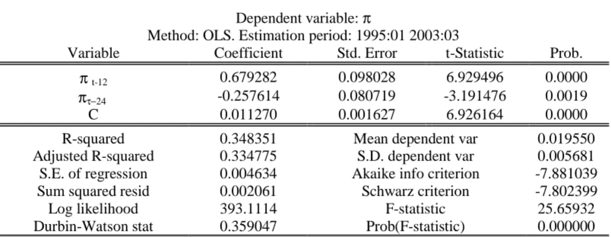
One simple way to assess the autocorrelation of inflation rates is to estimate equation (9) using monthly data. In order to consider monthly results, we look at the relationship between the current inflation rate over twelve months and past inflation rates over twelve-month periods that do not overlap (see Crawford, 2001, for example):

t t t t a

φ

π

φ

π

ε

π

= 0 + 1. ₋12 + 2. ₋24 + ) ' 10 (

The results are shown in Table 2. The estimated values of the parameters relating to lagged inflation are significantly different from zero. More specifically, the first autocorrelation coefficient, measured one year ahead, is positive, while the second, measured two years ahead, is negative. This pattern corresponds to a situation where the ECB is trying to bring the inflation rate back in line with its target within two years. This objective can be estimated by rewriting the equation as follows:

t t t t

φ

φ

π

φ

π

φ

π

ε

π

=(1− 1− 2) *+ 1. ₋12+ 2. ₋24 + ) ' (10'

where

π

*

is the steady-state inflation rate, which can also be seen as the medium-term inflation target.

Its estimated value,17_{in view of the results shown in Table 2, is equal to 1.94%.18 This is in line with}

the ECB’s announcement that it would maintain the inflation rate close to, but below, 2%.

Table 2

Dependent variable:π

Method: OLS. Estimation period: 1995:01 2003:03

Variable Coefficient Std. Error t-Statistic Prob.

π t-12 0.679282 0.098028 6.929496 0.0000

πτ−24 -0.257614 0.080719 -3.191476 0.0019

C 0.011270 0.001627 6.926164 0.0000

R-squared 0.348351 Mean dependent var 0.019550

Adjusted R-squared 0.334775 S.D. dependent var 0.005681

S.E. of regression 0.004634 Akaike info criterion -7.881039

Sum squared resid 0.002061 Schwarz criterion -7.802399

Log likelihood 393.1114 F-statistic 25.65932

Durbin-Watson stat 0.359047 Prob(F-statistic) 0.000000

Empirical studies on a number of countries show that persistence varies over time depending on the nature of monetary policy.19 What does observation of the euro area show? Have the creation of the ECB and the implementation of its price-stability-oriented monetary policy strategy had an impact on the autocorrelation of inflation rates? A comparison between the period from 1993 to 1998 and the period from 1999 to 2003 can provide some helpful information on the subject, even though there are obvious limitations. It would be simplistic to attribute all changes to the new monetary regime, since other factors, such as the change in exogenous shocks affecting inflation, could be involved too. Other factors might include economic agents’ anticipation of the regime change long before it came into effect. Chart 8, which plots the autocorrelation of inflation rates over each of the two periods, shows two changes. Overall, persistence seems to have diminished. The autocorrelation coefficient is weaker with each successive lag. The autocorrelation coefficient has become negative in the recent period for lags of one and a half years up to two years. This confirms an earlier observation and its interpretation as showing the ECB’s determination to bring the inflation rate back in line with its target within two years.

17π_{*, the steady-state inflation rate is derived from:}

2 1 *

1

ϕ

ϕ

π

−

−

=

C

18_{In view of the margin of error on the constant alone, the 95% confidence interval is [1.4% to 2.5%].}

19 _{For example, Longworth (2002) shows that the dynamic behaviour of Canadian inflation underwent fundamental changes after the}

Chart 8

Autocorrelation (y ear-on-year change in euro area HICP)

-0.4 -0.2 0 0.2 0.4 0.6 0.8 1 1 2 3 4 5 6 7 8 9 10 11 12 13 14 15 16 17 18 19 20 21 22 23 24 1993-1998 1999-2003

In order to make sure that this result is meaningful, we compare the value of the coefficients for successive lagged inflation rates over two sub periods (Chart 9) and the 95% confidence intervals around the estimated values of these coefficients (Chart 10).

Chart 9

Coefficients estimated by linear regression (current inflation over past inflation)

Estimated coefficients -0.4 -0.2 0 0.2 0.4 0.6 0.8 1 1 2 3 4 5 6 7 8 9 10 11 12 1993-1998 1999-2003

Chart 10

Confidence intervals around the coefficients 95% confidence intervals -0.8 -0.6 -0.4 -0.2 0 0.2 0.4 0.6 0.8 1 1.2 1 2 3 4 5 6 7 8 9 10 11 12 1993-1998 1999-2003

These two charts show that it is very difficult to distinguish between the two sub-periods at the statistical level. With a few rare exceptions, the value of the coefficient hardly changes from one period to the next and the 95% confidence intervals are practically indistinguishable. Furthermore, these coefficients are not statistically different from zero.

2.3.4. Short-term price-level uncertainty

Uncertainty about short-term inflation can first be measured by the conditional variance of forecasting errors derived from a generalised autoregressive conditional heteroscedastisity model of inflation20

(Crawford and Kasumovich, 1996; Jenkins and O’Reilly, 2001; Longworth, 2002). Such a measure constructed for the euro area on the basis of a GARCH(1.1) model estimated for the period from 1993 to 2003 produces the following results:

Chart 11

Uncertainty about inflation (HICP)

(conditional variance) . 0 8 . 1 0 . 1 2 . 1 4 . 1 6 . 1 8 9 3 9 4 9 5 9 6 9 7 9 8 9 9 0 0 0 1 0 2

20_{In this type of model, the expected variance of inflation for the following period, which is also called conditional variance, is assumed to}

depend on three terms: mean inflation, new information about volatility obtained during the previous period and measured as the square of the forecasting error, and past variance forecasts.

Uncertainty about inflation during the period under review seems to stabilise at low levels at the end of the nineteen-nineties. It then increases rapidly, concomitantly with energy price shocks and unprocessed food price shocks, and again with the changeover to the euro. At the very end of the period, when uncertainty seems to ease and return to its earlier levels, the rise in oil prices brings with it a fresh surge in uncertainty. The estimation of the GARCH model also shows how highly entrenched the impact of shocks on inflation volatility is, as the autoregressive root corresponding to the sum of the coefficients on the ARCH and GARCH terms is close to unity (0.88).

We can use a second type of indicator, which is based on the dispersion of inflation forecasts according to the time horizon for the forecast. Chart 12 below shows this indicator, which is derived from the ECB’s Survey of Professional Forecasters mentioned above. As we can see in Chart 12, the dispersion naturally tends to increase as the time horizon grows more distant. The variance of forecasts four years ahead (n+4), two years ahead (or eight quarters, denoted q+8) and one year ahead is generally greater than the variance of forecasts relating to the current year is. However, there is a steady diminishing trend in the dispersion of inflation forecasts four years ahead, which could be interpreted as a sign of reduced uncertainty about the short- to medium-term inflation rate. This trend corroborates the conclusions drawn on the basis of the preceding indicator to a certain extent.

Chart 12 E C B S u r v e y s o f P r o fe s s io n a l F o r e c a s t e r s : s t a n d a r d d e v ia t io n -0 .1 0 .2 0 .3 0 .4 0 .5 0 .6 1 9 9 9 q 1 1 9 9 9 q 3 2 0 0 0 q 1 2 0 0 0 q 3 2 0 0 1 q 1 2 0 0 1 q 3 2 0 0 2 q 1 2 0 0 2 q 3 2 0 0 3 q 1 n n + 1 n + 4 q + 8

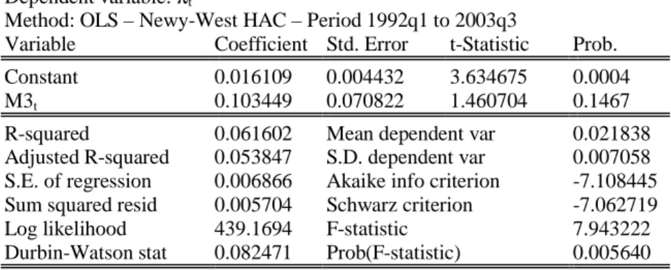
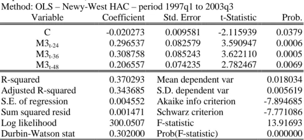
2.3.5. Information provided by money

Even though the New Keynesian analytical framework seems to attribute it a limited role, money can still be useful for monetary decision-making because of its information content with regard to future activity and inflation.

Tables 3 and 4 below show some empirical results obtained from an analysis based on the approach originally proposed by Stock and Watson (2001), where the predictive powers of some fifty potential leading indicators are assessed with regard to future activity and inflation in the euro area. The indicators assessed include certain commodity prices, a vast assortment of asset prices and financial variables, a measure of the output gap and, finally, monetary aggregates. The estimates are made for the period from 1980 to 2002. The quality of a leading indicator is measured on the basis of its predictive powers two, four and eight quarters ahead. The tables show the Relative Root Mean Square Error (Relative RMSE) of the forecasts made without samples and obtained with the help of a purely autoregressive model of activity growth and inflation and those obtained using a model that incorporates current and past values of the leading indicator under consideration. A ratio of less than 1 shows that the indicator contains information about future activity or inflation, since taking it into