The Asteroseismic Target List for Solar-like Oscillators Observed in 2 minute Cadence with the Transiting Exoplanet Survey Satellite

(1)

HAL Id: hal-02105120

https://hal.archives-ouvertes.fr/hal-02105120

Submitted on 20 Apr 2019

HAL is a multi-disciplinary open access

archive for the deposit and dissemination of

sci-entific research documents, whether they are

pub-lished or not. The documents may come from

teaching and research institutions in France or

abroad, or from public or private research centers.

L’archive ouverte pluridisciplinaire HAL, est

destinée au dépôt et à la diffusion de documents

scientifiques de niveau recherche, publiés ou non,

émanant des établissements d’enseignement et de

recherche français ou étrangers, des laboratoires

publics ou privés.

The Asteroseismic Target List for Solar-like Oscillators

Observed in 2 minute Cadence with the Transiting

Exoplanet Survey Satellite

Mathew Schofield, William Chaplin, Daniel Huber, Tiago Campante, Guy

Davies, Andrea Miglio, Warrick Ball, Thierry Appourchaux, Sarbani Basu,

Timothy Bedding, et al.

To cite this version:

Mathew Schofield, William Chaplin, Daniel Huber, Tiago Campante, Guy Davies, et al.. The

As-teroseismic Target List for Solar-like Oscillators Observed in 2 minute Cadence with the Transiting

Exoplanet Survey Satellite. Astrophysical Journal Supplement, American Astronomical Society, 2019,

241 (1), pp.12. �10.3847/1538-4365/ab04f5�. �hal-02105120�

(2)

The Asteroseismic Target List for Solar-like Oscillators Observed in 2 minute Cadence

with the Transiting Exoplanet Survey Satellite

Mathew Schoﬁeld1,2 , William J. Chaplin1,2 , Daniel Huber3 , Tiago L. Campante1,4,5 , Guy R. Davies1,2 , Andrea Miglio1,2 , Warrick H. Ball1,2 , Thierry Appourchaux6 , Sarbani Basu7 , Timothy R. Bedding2,8 , Jørgen Christensen-Dalsgaard2 , Orlagh Creevey9 , Rafael A. García10, Rasmus Handberg2, Steven D. Kawaler11 , Hans Kjeldsen2, David W. Latham12 , Mikkel N. Lund2 , Travis S. Metcalfe13,14 , George R. Ricker15, Aldo Serenelli16,17,

Victor Silva Aguirre2 , Dennis Stello2,8,18 , and Roland Vanderspek15

1

School of Physics and Astronomy, University of Birmingham, Birmingham B15 2TT, UK;w.j.chaplin@bham.ac.uk

2

Stellar Astrophysics Centre(SAC), Department of Physics and Astronomy, Aarhus University, Ny Munkegade 120, DK-8000 Aarhus C, Denmark

3

Institute for Astronomy, University of Hawai‘i, 2680 Woodlawn Drive, Honolulu, HI 96822, USA

4

Instituto de Astrofísica e Ciências do Espaço, Universidade do Porto, Rua das Estrelas, PT4150-762 Porto, Portugal

5

Departamento de Física e Astronomia, Faculdade de Ciências da Universidade do Porto, Rua do Campo Alegre, s/n, PT4169-007 Porto, Portugal

6_{Université Paris-Sud, Institut d’Astrophysique Spatiale, UMR 8617, CNRS, Bâtiment 121, F-91405 Orsay Cedex, France} 7

Department of Astronomy, Yale University, P.O. Box 208101, New Haven, CT 06520-8101, USA

8

Sydney Institute for Astronomy(SIfA), School of Physics, 2006 University of Sydney, Australia

9

Université Côe d’Azur, Observatoire de la Côte d’Azur, CNRS, Laboratoire Lagrange, Bd de l’Observatoire, CS 34229, F-06304, Nice Cedex 4, France

10_{Laboratoire AIM, CEA/DSM-CNRS—Univ. Paris Diderot-IRFU/SAp, Centre de Saclay F-91191 Gif-sur-Yvette Cedex, France} 11

Department of Physics and Astronomy, Iowa State University, Ames, IA 50011, USA

12

Harvard-Smithsonian Center for Astrophysics, 60 Garden Street, Cambridge, MA 02138, USA

13

Space Science Institute, 4750 Walnut Street, Suite 205, Boulder, CO 80301, USA

14

Max-Planck-Institut für Sonnensystemforschung, Justus-von-Liebig-Weg 3, D-37077, Göttingen, Germany

15

MIT Kavli Institute for Astrophysics and Space Research, 70 Vassar Street, Cambridge, MA 02139, USA

16

Institute of Space Sciences(ICE, CSIC) Campus UAB, Carrer de Can Magrans s/n, E-08193 Barcelona, Spain

17_{Institut d’Estudis Espacials de Catalunya (IEEC), C/Gran Capità, 2-4, E-08034 Barcelona, Spain} 18

School of Physics, UNSW Sydney, NSW, 2052, Australia

Received 2018 November 15; revised 2019 January 9; accepted 2019 January 24; published 2019 March 14

Abstract

We present the target list of solar-type stars to be observed in short-cadence(2 minute) for asteroseismology by the NASA Transiting Exoplanet Survey Satellite (TESS) during its 2 year nominal survey mission. The solar-like Asteroseismic Target List(ATL) is comprised of bright, cool main-sequence and subgiant stars and forms part of the larger target list of the TESS Asteroseismic Science Consortium. The ATL uses the Gaia Data Release 2 and the Extended Hipparcos Compilation (XHIP) to derive fundamental stellar properties, to calculate detection probabilities, and to produce a rank-ordered target list. We provide a detailed description of how the ATL was produced and calculate expected yields for solar-like oscillators based on the nominal photometric performance by TESS. We also provide a publicly available source code that can be used to reproduce the ATL, thereby enabling comparisons of asteroseismic results from TESS with predictions from synthetic stellar populations.

Key words: catalogs– space vehicles: instruments – stars: fundamental parameters – stars: oscillations – surveys Supporting material: machine-readable table

1. Introduction

NASA’s Transiting Exoplanet Survey Satellite (TESS) was launched on 2018 April 18 with the main goal to detect small planets orbiting nearby stars using the transit method (Ricker et al.2014). Its photometric data will also enable high-fidelity studies of stars and other astrophysical objects and phenomena (e.g., transients, galaxies, solar system objects, etc.). TESS is observing bright stars, including those visible to the naked eye, opening up a new discovery space to characterize stars several magnitudes brighter than those observed by the NASA Kepler Mission. While Kepler(Borucki et al.2010) and its repurposed follow-up mission known as K2(Howell et al.2014) observed stars in only dedicatedfields, TESS will survey over 85% of the sky during its 2 year nominal mission,19 covering first the southern and then the northern equatorial hemispheres(e.g., see Huang et al. 2018). TESS thus promises to provide a unique census of bright stars in the solar neighborhood.

TESS will produce full-frame image (FFI) data every 30 minute for the entire ﬁeld of view (FOV), and 2 minute (short-cadence) data on a total of approximately 200,000 targets. The short-cadence target list is comprised of several cohorts: high-priority targets for exoplanet transit searches, which form the Candidate Target List (CTL; Stassun et al. 2018) targets from the TESS Guest Investigator (GI) program;20 the Directorʼs Discretionary Target (DDT) and out-of-cycle Target of Opportunity (ToO) programs;21 and targets for asteroseismic studies of stars(e.g., Chaplin & Miglio2013).

The high-precision, high-cadence, near continuous photo-metric data that TESS will provide are well suited to asteroseismology. As with Kepler (Gilliland et al. 2010), the international asteroseismology community is coordinating efforts through the TESS Asteroseismic Science Consortium (TASC).22 _{Owing to their short oscillation periods, there are} The Astrophysical Journal Supplement Series, 241:12 (10pp), 2019 March https://doi.org/10.3847/1538-4365/ab04f5

19 https://heasarc.gsfc.nasa.gov/docs/tess/ 20 https://heasarc.gsfc.nasa.gov/docs/tess/proposing-investigations.html 21_{https://tess.mit.edu/science/ddt/} 22 http://tasoc.dk

(3)

several classes of stars that require short-cadence data for asteroseismology. The most prominent examples are solar-type stars, which are here deﬁned as cool main-sequence and subgiant stars that show solar-like oscillations that are stochastically excited and intrinsically damped by near-surface convection. Kepler and K2 have provided asteroseismic detections in approximately 700 solar-type stars (Chaplin et al. 2011b, 2014; Lund et al. 2016b), including about 100 Kepler planet hosts(Huber et al.2013; Lundkvist et al.2016). The main limitation for the asteroseismic yield of Kepler/K2 was the limited number of short-cadence target slots; there were around 500 available at any one time to the mission. That constraint will be eased dramatically for TESS, giving the potential to provide detections for thousands of solar-type stars. In addition to asteroseismic characterizations of already known planet hosts (Campante et al. 2016), TASC will also provide the TESS Science Team with such data on the bright solar-type hosts around which TESS will discover planets.

TESS will dedicate around 20,000 short-cadence targets to asteroseismology, and it is the responsibility of TASC to provide the target list. In this paper we describe the construction of the prioritized Asteroseismic Target List (ATL) of solar-like oscillators, which forms part of the overall TASC list. The breakdown of the rest of the paper is as follows. We begin in Section 2 by describing the basic philosophy underlying the construction of the ATL. Section3summarizes the input data. In Section 4, we discuss in detail the steps followed to produce a prioritized target list. Then in Section5, we provide an overview of the rank-ordered list, including a prediction of the overall asteroseismic yield. We ﬁnish in Section 6 with a summary overview of the list, including information on how to access both the ATL in electronic form23 and the Python codes used to construct it in a Github repository.24

2. Philosophy for the Construction of the ATL Our goal was to produce an all-sky rank-ordered target list based on basic observables from all-sky catalogs and derived quantities that can be easily be duplicated for simulated populations(to facilitate stellar populations studies). The most obvious approach would be to select stars that are expected to show solar-like oscillations (i.e., stars cool enough to have convective envelopes) and then to rank by the apparent magnitude (either in the TESS bandpass, T, or the Johnson I band, which is a good proxy of the TESS magnitude). However, we must also consider whether solar-like oscillations are likely to be detected in a potential target. This requires a prediction of expected photometric amplitudes of the solar-like oscillations, stellar granulation, and the expected shot and instrumental noise. A simple rank-order approach based on the apparent magnitude would signiﬁcantly compromise the potential yield of asteroseismic detections and omit targets for which we expect to make asteroseismic detections.

We, therefore, base the ranking in our list on predictions of asteroseismic detectability, which were made using the basic methodology developed for and applied successfully to Kepler target selection (Chaplin et al.2011a). While this approach is more complicated, it is worth stressing that the asteroseismic predictions use simple analytical formulae, which may be

applied straightforwardly to synthetic populations. All codes and data used to produce the target list are publicly available to facilitate reproducibility and the comparison with synthetic stellar populations.

3. Input Data 3.1. Input Catalogs

The ATL is mainly based on targets in Gaia Data Release 2 (DR2)25 _{(Gaia Collaboration et al.} ₂₀₁₈_{), supplemented at}

bright magnitudes by the eXtended Hipparcos Compilation (XHIP; Anderson & Francis2012). The basic set of data used to construct the ATL comprises the astrometric distances, magnitudes in the I and V bands, the (B−V ) color, and the sky positions. From these input data, we may estimate the photometric variability in the TESS bandpass caused by solar-like oscillations, granulation, and shot/instrumental noise, as well as the expected duration of the TESS observations. Using these derived quantities, we then calculate the probability of detecting solar-like oscillations.

3.2. Fundamental Stellar Properties

Distances for Gaia DR2 stars were taken from Bailer-Jones et al.(2018) using the median of the posterior calculated using their Milky Way prior. This set of distances was chosen because the Milky Way prior performs better for stars closer than 2 kpc, where the vast majority of the ATL targets are located. Distances for XHIP stars were derived by inverting the parallax. We added a zeropoint offset of 0.029 mas to all Gaia DR2 parallaxes(Luri et al.2018; Zinn et al.2018). After this, we discarded all targets in both catalogs that have a fractional parallax uncertaintyσ_π/π>0.5. Reddening and extinction in the V and I bands were calculated from the derived distances and sky positions(Galactic coordinates) using the Combined15 dust map from theMWDUST Python package(Drimmel et al. 2003; Marshall et al. 2006; Green et al. 2015; Bovy et al.

2016).

While I-band magnitudes are available for XHIP targets, this is not the case for most of the Gaia DR2 targets. This is important because the I magnitudes are needed to estimate the shot noise in the TESS bandpass. We, therefore, used(B−V ) colors and apparent V magnitudes to derive the required values. The preferred source for both inputs was the revised Hipparcos catalog(van Leeuwen2007). If those data were unavailable, we used the Tycho-2 catalog (Hog et al. 2000); failing that, we took values from the American Association of Variable Star Observers (AAVSO) All-Sky Photometric Survey (Henden et al.2009).

The input (B−V ) colors were first dereddened using the previously calculated E(B−V) and then converted to (V−I) using the polynomials in Caldwell et al. (1993). The coefficients of the polynomial depend upon whether the target is classified as a “giant” or “dwarf.” Here, we separated targets using an empirically derived relation in Mg, the absolute

magnitude in the Gaia bandpass, and (B−V ), using DR2 data, classifying stars with Mg>6.5×(B−V )−1.8 as

dwarfs, and the rest as giants. Once(V−I) had been calculated for all of the stars, the I magnitudes were estimated from V and (V−I). The derived I magnitudes were then reddened using

23_{https://ﬁgshare.com/s/aef960a15cbe6961aead} 24

(4)

the previously estimated AI to calculate the TESS noise (see

Section 4).

Dereddened (B−V ) colors were used to estimate stellar effective temperatures, Teff, using color–temperature relations

of the form:26

T a b B V c B V

log( eff)= + ( - )+ ( - )2+..., ( )1 where the best-ﬁtting coefﬁcients were taken from Torres (2010). Luminosities, L, were calculated from

L L M V A log 4.0 0.4 2.0 log 0.4 V BC .V 2 bol mag p = + -- - +   ( ) ( ) ( )

Note that V magnitudes were ﬁrst dereddened using the previously calculated AV, while the bolometric corrections,

BCV, were taken from Flower (1996), as presented in Torres

(2010), with M_bol,e=4.73±0.03 mag. Finally, we estimated radii using the Stefan–Boltzmann law L R T2

eff 4

µ , with

T_eff,e=5777 K.

3.3. Comparison to Literature Values

We compared our estimated stellar properties with several literature sources. The PASTEL catalog(Soubiran et al.2016) includes spectroscopically determined effective temperatures for over 60,000 stars. Figure 1 compares our derived photometric temperatures with PASTEL for stars that are common to both lists. We observe good agreement, with a residual median and scatter of 102 K and 146 K, respectively. We furthermore compared our temperatures with values listed in Huang et al.(2015), which compiled empirical temperatures derived from optical long-baseline interferometry (e.g., Mozurkewich et al.2003; Boyajian et al.2012a,2012b,2013). Figure2again shows good agreement, with a residual median and scatter of 109 K and 173 K, respectively. Both comparisons show that our temperatures are, on average, ∼100 K hotter, which is comparable to previously found offsets between

temperature scales(Pinsonneault et al.2012) and is well within the systematic uncertainty of the fundamental interferometric temperature scale itself(e.g., White et al.2018). Based on these comparisons, we have adopted a conservative uncertainty of 3% on the temperatures in the ATL, which encompasses both random and systematic uncertainties from the literature comparisons.

Next, we compared radii in the ATL to a selection of bright stars in Silva Aguirre et al. (2012) and Bruntt et al. (2010). Silva Aguirre et al.(2012) derived radii for a small number of Kepler solar-type stars that have detections of solar-like oscillations, as well as precise Hipparcos parallaxes. Bruntt et al.(2010) estimated the radii of even brighter stars using two approaches:ﬁrst, using measurements of limb-darkened stellar angular diameters and stellar parallaxes; and second, using the Stefan–Boltzmann law with luminosities derived from V-band magnitudes, bolometric corrections and parallaxes, and spectro-scopic temperatures, i.e., the basic approach we have used but with some different observables. Figure 3 shows the compar-ison with between ATL and those literature values. We observe excellent agreement, with a residual median and scatter of 4% and 7%, respectively. Overall, these comparisons conﬁrm that the stellar properties derived in the ATL do not suffer from large systematic errors when compared with literature values.

Figure 1. Comparison between effective temperatures from high-resolution spectroscopy (as listed in the PASTEL catalog) and the ATL photometric temperatures. The solid line shows the 1:1 relation. The horizontal lines of data points exist because the PASTEL catalog gives several effective temperatures for some stars. The residual median and scatter is 102 K and 146 K, respectively.

Figure 2. Comparison between effective temperatures from long-baseline interferometry(as compiled by Huang et al.2015) and the ATL. The solid line

shows the 1:1 relation. The residual median and scatter are 109 K and 173 K, respectively.

Figure 3.Comparison between the literature radii derived from parallaxes(red and blue symbols) and interferometry (green symbols). We observe good agreement, with a residual median and scatter of 0.04% and 0.07%.

26

We adopt relations that do not include any correction for metallicity, as we do not have good/uniform quality estimates of [Fe/H] for all targets under consideration.

(5)

4. ATL Construction

4.1. Consolidation of DR2 and XHIP Entries

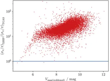
Having removed stars with large fractional parallax uncertainties(see Section3.2), we combined the retained stars from DR2 and XHIP into a single list to be treated homogeneously. This combined list contained over 300,000 stars. Most had entries in the DR2 catalog, with only a small number in XHIP. However, there were ∼17,000 stars that existed in both lists. We broke this degeneracy using data and derived parameters from the catalog whose target entry had the smaller fractional parallax uncertainty of the two. Not surprisingly, in the vast majority of cases, the DR2 entries were selected, with only a handful of bright XHIP targets being retained where Hipparcos outperforms Gaia (see Figure4).

4.2. Down-selection to Solar-like Oscillating Short-cadence Targets

From the above combined list, we selected targets that are potential solar-like oscillators. To do this, we retained all stars that lie on the cool side(redward) of the δ Scuti instability strip, i.e., those that have Teff<Tred, with the red-edge temperature

deﬁned, as Chaplin et al. (2011a):

Tred=8907 K´(L L)-0.093. ( )3 We further restricted to targets that have predicted dominant oscillation frequencies requiring the TESS short-cadence (2 minute) data. Solar-like oscillators present a rich spectrum of detectable overtones, with oscillation power following a Gaussian-like envelope centered on the so-called frequency of maximum oscillations power,νmax. We retained all targets that

have νmax240 μHz. This represents, to a reasonable

approximation, an upper limit cut in the luminosity that discards low-luminosity red-giants at or just above the base of the red-giant branch, i.e., giants whose solar-like oscillations can be very readily resolved in the TESS 30 minute long-cadence FFI data. The 240μHz limit was set deliberately to lie below the FFI Nyquist frequency of 278μHz to account for uncertainties in the ATL-based predictions and also to provide a reasonable sample of targets in short-cadence whose

oscillation spectra are reasonably close to the Nyquist limit. Experience from Kepler has shown that such spectra can be difﬁcult to analyze using long-cadence data only, due to aliasing about the Nyquist frequency(e.g., Yu et al.2016).

The boundary in the L–Teff plane for the νmax cut follows

from the approximate relation(see Campante et al.2016): R R T T , 4 max max, 1.85 eff eff, 0.92 n =n -   ⎛ ⎝ ⎜ ⎞ ⎠ ⎟ ⎛ ⎝ ⎜ ⎞ ⎠ ⎟ ( )

which, combined with L R T2 eff4

µ and settingνmax=240 μHz,

deﬁnes the boundary

L L T T 16.7 eff 5 eff, 5  ´   ⎛ ⎝ ⎜ ⎞ ⎠ ⎟ ( )

for retaining targets. Figure 5 shows the I magnitude distribution of the Hipparcos and Gaia subsamples of the ATL after these Hertzsprung–Russell (H–R) diagram cuts have been applied. As expected, Gaia dominates the faint end of the ATL, and the drop-off at I∼11 is caused by the fractional parallax precision cut described in Section3.2.

4.3. Estimation of Asteroseismic Detection Probabilities To calculate asteroseismic detection probabilities, we used the approach developed by Chaplin et al.(2011a), which has been applied successfully to short-cadence target selection for Kepler Objects of Interest in the Kepler nominal mission and, more recently, to short-cadence target selection for solar-type stars observed with K2 (e.g., see Chaplin et al. 2015; Lund et al.2016a,2016b). The approach is based on predicting the global signal-to-noise ratio (S/N) in the oscillation spectrum, i.e., the predicted total power in the observed solar-like oscillations divided by the total power from granulation and shot and instrumental noise, summed across the range in the frequency occupied by the modes. The total oscillation and granulation power across the frequency range of interest centered on the predicted νmax may be calculated from the

previously derived L, Teff, and R. The shot and instrumental

noise depend on the instrumental performance and the apparent magnitude of targets in the instrumental bandpass. The duration of the observations is also an important factor: at a given global

Figure 4.Stars with both DR2 and XHIP entries. The fractional parallaxσπ/π

value was calculated from the DR2 and XHIP entries for each star separately. The parameters from the catalog with the lowerσπ/π value was chosen. XHIP

properties were only used for the few stars below the blue line.

Figure 5. Imagdistribution of the XHIP and DR2 catalogs, shown here after

Teff/L cuts, but before Pdetwas calculated. The inset shows the Imag region

(6)

S/N, the detection probability will rise as the length of observations is increased.

The formulation by Chaplin et al. (2011a) was updated for the TESS instrumental speciﬁcations in Campante et al. (2016). We followed that revised recipe in detail here and refer the reader to Section3 of Campante et al. (2016) for the relevant steps and relations. We have made some changes to the estimation of the TESS noise to reﬂect updates to information that is available on the instrumental performance. We describe those small changes next in Section 4.3.1.

4.3.1. Updates to Noise Predictions

The predicted instrumental noise is dominated by the shot noise, but also includes contributions to represent contamina-tion from nearby stars and readout noise. Since the ATL targets are bright, contamination is expected to be modest, in spite of the large point-spread function of TESS. Note that we assumed that the systematic noise ﬂoor of 60 ppm per hour (Sullivan et al. 2015) is negligible, as this is a design threshold requirement to meet core exoplanet science deliverables and will not reﬂect the actual performance.

As in Campante et al. (2016), we used the calc_noise IDL procedure provided by the TESS Science Team (Sullivan et al.2015) to calculate the instrumental noise, which takes the I-band magnitude as its main input. There are two updates:(i) the absolute calibration of the expected noise levels is now slightly higher, due to a reduced estimated effective aperture size for the instrument; and(ii) the expected number of pixels, Nmask, in each stellar pixel mask is now smaller, which has the

effect of reducing noise levels. Updated mask sizes were calculated using the simple parametric model provided by the TESS team(J. Winn 2019, private communication):

N 10 I , 6

mask= 0.8464-0.2144´(mag-10.0) ( )

and the number of pixels was rounded up to the nearest whole number. Once calculated, the individual instrumental noise contributions(see Figure6) were summed in quadrature to give the total instrumental noise per 2 minute cadence.

4.3.2. The Observation Time in the TESS FOV

We begin this section with a recap of the basic information on the TESS FOV and observing strategy(see also, e.g., Ricker et al. 2014; Sullivan et al. 2015; Huang et al. 2018). TESS comprises four CCD cameras. Each CCD images a 24°×24° area on the sky, with the total collecting area of the four cameras at any given time being a strip of dimensions 24° (ecliptic longitude)×96° (ecliptic latitude). TESS will survey the sky south of the ecliptic in its ﬁrst year of science operations, with the hemisphere divided into 13 strips. Each resulting pointing will last, on average, about 27.4 days. The durations of each sector pointing differ by up to 1.5 days due to variations in the length of the spacecraft’s orbit. The sky north of the ecliptic will be observed in the second year of nominal science operations.

The majority of TESS targets will be observed over only one 27-day sector. The duration increases for latitudes signiﬁcantly above or below the ecliptic plane, because targets may then be observed in more than one sector pointing, reaching a maximum of 13 sectors, i.e., about 351 days, at the ecliptic poles (the continuous viewing zone, see Figure7). TESS will not observe targets within ±6° of the ecliptic during its nominal mission, and those stars were removed from our list.

Figure7shows that there will be small gaps between sectors. At the time the ATL was delivered, the initial pointing at the commencement of science operations was not known. As can be seen from the ﬁgures, that will inﬂuence not only which stars are missed by TESS (i.e., those falling in the sector-to-sector gaps at low ecliptic latitudes), but also the number of sectors for which targets at higher latitudes will be observed. Here, we ignore the low-latitude gaps and assume that all stars with ecliptic latitudes beyond ±6° are potentially observable. Targets that fall in the gaps will be discarded when the TESS team compiles actual target lists for each known pointing.

For higher-latitude targets, there are several options open to us. We could adopt a particular pointing and then compute the resulting number of observation sectors for each target for input to the asteroseismic detection recipe. We could instead estimate the minimum and maximum potential number of observation sectors for each target, which depend on the ecliptic latitude but

Figure 6.Individual noise contributions(colored lines) and total noise budget (black line) as a function of the apparent I magnitude used to calculate asteroseismic detection probabilities.

Figure 7.FOV from one of the ecliptic poles. The color bar represents how long a part of the sky will be observed by TESS. The dotted circles are lines of constant latitude(0°, 30°, and 60°). The center of the image has a latitude of 90°. The outer dotted circle at 0° latitude has labels for 0° and 180° longitude. The horizontal dotted line represents longitude values of 0° and 180°. The Astrophysical Journal Supplement Series, 241:12 (10pp), 2019 March Schoﬁeld et al.

(7)

not the exact pointing, and use one or the other as input to the detection recipe. While this choice will affect the rank ordering of targets based on the detection probability, it turns out that the resulting changes in ranking are typically a few hundred places or less, a change that is very unlikely to inﬂuence whether targets with potentially detectable oscillations are observed by TESS. As such we adopted the simplerﬁrst option and assumed an initial pointing of Elong=0°.

The ecliptic position(Elong, Elat) determines how long a star

can be observed. To determine whether a star is observable in any given sector pointing, we must deﬁne the longitudes of the center of each observing sector, ECCD, and the longitude range,

frange, that the cameras cover at a given latitude (i.e., the

latitude of the star). Figure8gives a pictorial representation of frange. The black circle in Figure8is a line of constant latitude.

In Figure8, the satellite is represented by the small red circle in the center of the image. The red dashed lines show the width of the FOV of TESS. These are the edges of frange.

frangeis given by E 24 cos , 7 range lat f =  ( ) ( )

where Elatis the latitude of the star in question, and 24° is the

width of theﬁeld covered by the CCD cameras at 0° latitude. If the longitude of the star lies within ±frange/2, then the image

of the star will be captured by a camera. In order to check this, the difference between the center of the CCD (ECCD) and the

longitude of the star(Elong) must be calculated. This difference

is given by E E E E , 360 . 8 Diff CCD long CCD long f = - - -⎧ ⎨ ⎩ ∣ ∣ ∣ ∣ ( )

Equation(8) will produce two values of fDiff, as shown by

the blue and green lines in Figure8. Only the smaller distance between Elong and ECCD should be taken as the distance

between the star and the center of the FOV. The longitudinal position of a star is marked in Figure8by the orange line.

Now, if frangefDiff, the star will be observed in that

region. In Figure 8, the length of the blue arc will be the accepted value forfDiff, because it is shorter than the green arc.

However, although the blue arc is the shorter of the two, frange<fDiff, and so the star will not be observed in this

sector.

Using Equations (7) and (8), we determined which stars would be observable in theﬁrst sector pointing of each ecliptic hemisphere, again taking each to be centered on ECCD=0°.

The same calculations were then repeated for each subsequent pointing, with every adjacent pointing shifted by ECCD=360°/13=27°.7. The observing time Tobs was then

obtained from the maximum contiguous number of sectors that each star is observed.

4.3.3. Rank Ordering the ATL Using the Detection Probabilities The analysis of the Kepler sample demonstrated that amplitudes of solar-like oscillations are progressively reduced relative to predictions from scaling relations when moving from late to early F-type stars. Chaplin et al.(2011a) attempted to capture this effect explicitly by introducing an attenuation factor,β, which was also adopted by Campante et al. (2016) to describe the maximum amplitude for radial mode oscillations in the TESS bandpass:

A R R T T 0.85 2.5 ppm . 9 max 1.85 eff eff, 0.57 b = ´ ´ ´ ´   ⎛ ⎝ ⎜ ⎞ ⎠ ⎟ ⎛ ⎝ ⎜ ⎞ ⎠ ⎟ ( )

Here,β is given by:

T T

1.0 exp red eff 1550 K , 10

b = - [( - ) ] ( )

where Tred is the previously deﬁned temperature on the red

edge of the δ Scuti instability strip at the luminosity of the target (see Equation (3)). The attenuation given by β reduces predicted mode amplitudes in hotter stars, and hence lowers detection probabilities and the associated rank ordering of those targets. Figure9illustrates the effect by showing all ATL stars with detection probabilities greater than 50% with and without including the β factor. As expected, the β factor strongly reduces the number of stars with signiﬁcant detection probabilities, especially toward the instability strip.

Rank ordering the ATL using the detection probabilities and including theβ factor would optimize the yield of asteroseismic detections with TESS. However, using theβ factor would also strongly bias against making new discoveries in stars that do not ﬁt the trend in asteroseismic amplitudes shown by the Kepler sample on which the detection recipe is based(that is, by deﬁnition, an already biased sample).

The group most affected by this is comprised of hot F-type stars, which lie at the boundary where solar-like oscillations diminish to undetectable amplitudes and classical pulsations driven by the κ mechanism start to become excited. Determining the details of this transition is of considerable interest for understanding the driving and damping of oscillations, and intriguing examples of“hybrid stars” showing signatures of solar-type oscillations and classical pulsators have already been detected (Kallinger & Matthews 2010; Antoci et al. 2011), leading to suggestions of new pulsation driving mechanisms (Antoci et al. 2014). The sampling of targets in

Figure 8.Example of what is calculated in order to determine whether a star lies inside frange. In this example, the star’s longitude (represented by the

orange line) lies outside of the satellite’s FOV, as marked by the red dashed lines(Equation (7)).

(8)

this region was sparse for Kepler and was limited by the small number of short-cadence target slots available at any one time. There is now the potential to address those issues with TESS.

To mitigate the strong bias against hot stars in the ATL, we deﬁne a new probability, pmix, as follows:

p_mix =(1-a)p_vary +ap_fix. (11) Here, pvaryis the detection probability calculated using the β

factor, p_fix is the detection probability calculated by fixing β=1 for all stars (i.e., ignoring amplitude attenuation), and α regulates the relative weighting between pvary and pfix. After

investigating the rank-ordered lists using a range of values ofα, we found thatα=0.5 (i.e., equal weighting between pvaryand

p_ﬁx) provides the best overall compromise between obtaining a signiﬁcant yield and including enough hot stars at high ranks. For the remainder of the paper, all ranked lists in the ATL were calculated with detection probabilities using α=0.5.

5. Overview of the ATL

5.1. Distribution across the H–R Diagram

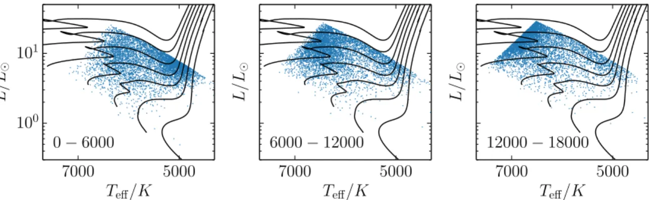
Figure 10 shows the distribution of the 18,000 top-ranked stars in the ATL in an H–R diagram, split into bins of 6000 stars each. Similar to Figure 9, the sharp edges are caused by the down-selection of solar-type dwarfs and subgiants using Equations (3) and (4). As expected, the top-ranked stars are dominated by cool, high-luminosity subgiants with intrinsically

high detection probabilities. Progressing toward lower ranks, a larger number of hot stars appear, which is a direct consequence of relaxing the β amplitude dilution factor described in Section4.3.3.

The distribution of targets in Figure 10 demonstrates the well-known bias of asteroseismic detections against cool, low-mass stars due to their intrinsically low oscillation amplitudes (see, e.g., Chaplin et al.2011a). In total, only six stars ranked among the top 25,000 in the ATL have luminosities less than solar. This makes the ATL highly complementary to the exoplanet target list, which prioritizes cool dwarfs due to the improved probability ofﬁnding small transiting exoplanets. We note that all solar-type stars that have a magnitude T<6 in the TESS bandpass are automatically included in the TESS 2 minute cadence target list(Stassun et al. 2018), irrespective of their position on the ATL.

5.2. Expected Yield

To estimate the expected yield of asteroseismic detections, we performed a Monte Carlo simulation as follows. For each star in the ATL, we drew a uniform random number n between zero and unity and counted the target as a potential seismic detection if n<pvary. We recall here that pvary provides a

conservative yield, because the amplitude dilution factorβ may be overestimated. To determine whether the target would be observed in 2 minute cadence, we adopted a starting ecliptic longitude of zero degrees for the ﬁrst observing sector and

Figure 9.H–R diagram of all ATL stars with detection probabilities greater than 50% with (left panel) and without (right panel) including the β factor, which accounts for the attenuation of oscillation amplitudes toward the red edge of the instability strip(dashed line). Solid lines show solar metallicity evolutionary tracks with masses from 0.8 Meto 2.0 Mein steps of 0.2 Me. Note that the sharp edges are due to cuts at the red edge of the instability strip(Equation (3)) and stars oscillating with

frequencies accessible with TESS FFI data(Equation (4)).

Figure 10.H–R diagram of stars in the ATL. Each panel shows 6000 stars according to their ranking. Black lines show evolutionary tracks with masses from 0.8 Me

to 2 Mein steps of 0.2 Me.

(9)

picked the top 450 targets (the per-sector allocation of TASC) in the ATL that fall on silicon in that sector. We then repeated this for each of the 13 sectors in the southern ecliptic hemisphere, adding new detections to the list each time.

The predicted TESS yield for the first full year of science operations, corresponding to Guest Investigator Cycle 1, is ∼2500 oscillating targets, which is already a five-fold increase over the yield from the Kepler mission. Of these detections, the majority are observed for a single sector(∼1500), while ∼200 targets are expected to be observed for 10 sectors or more. The second year of nominal science operations (Cycle 2) is expected to produce a similar yield, bringing the total expected number of detections to 5000 stars. We emphasize that these estimates only take into account stars on the ATL and ignore potential overlaps with other target lists(such as the CTL and Guest Investigator Program), which would result in a slightly higher yield. They also assume that our adopted noise model provides a good description of the actual, in-flight photometric precision.

Figure 11(a) compares the predicted asteroseismic yield of TESS to detections for dwarfs and subgiants from the Kepler mission (Chaplin et al.2014). As expected, the TESS yield is skewed toward evolved subgiants with intrinsically larger amplitudes and contains a smaller number of cool dwarfs(for which higher photometric precision is required for a detection). Importantly, Figure 11(b) demonstrates that the TESS detec-tions will be, on average, 4–5 mag brighter than Kepler, which follows from the difference in aperture size. Similar to the characterization of transiting exoplanets, this will enable signiﬁcantly more powerful complementary follow-up observa-tions, including measurements of angular diameters using optical long-baseline interferometry (which was only possible for a handful of Kepler dwarfs and subgiants Huber et al.2012; White et al. 2013). Overall this demonstrates that TESS will excel in a signiﬁcantly different parameter space than Kepler, in particular, for evolved subgiants that exhibit mixed modes that allow powerful constraints on the interior structure (e.g., Chaplin & Miglio 2013; Hekker & Christensen-Dalsgaard2016).

6. Summary and Conclusions

We have presented the construction of the ATL for solar-like oscillators to be observed in 2 minute cadence by the TESS Mission. The main characteristics of the ATL can be summarized as follows:

1. The ATL includes 25,000 bright main-sequence and subgiant stars that have at least a 5% probability of detecting solar-like oscillations with TESS. Detection probabilities were calculated from stellar properties estimated from colors, parallaxes, and apparent TESS magnitudes. The ranking of targets is based on a mixture of detection probability and the prioritization of hot stars, for which the oscillation amplitudes are poorly understood.

2. We have validated our derived stellar properties against spectroscopy, asteroseismology, and interferometry, ﬁnd-ing good agreement. In addition to the asteroseismic detection probabilities, the ATL provides a homogeneous catalog of stellar properties for bright solar-type stars observed by TESS.

3. Based on the nominal TESS photometric performance and the number of target slots assigned to the ATL, we expect that TESS will increase the number of solar-type stars with detected oscillations by an order of magnitude over Kepler. Most of the detections will be in evolved subgiants, with only a small number of detections in unevolved main-sequence stars.

4. ThePython code used to produce the ATL is publicly available on Github,27,28 allowing full reproducibility of the asteroseismic target selection for comparison with population synthesis models. The ATL itself is available in electronic form.29The columns of the ATL are shown in Table1.

Figure 11.Predicted asteroseismic yield for theﬁrst year of TESS science operations (Cycle 1). Panel (a): radius vs. effective temperature for all expected TESS detections(blue) and the detections for dwarfs and subgiants by Kepler (red). The blue dashed line marks the approximate radius limit above that oscillations can be conﬁdently detected using FFI light curves. Black lines show evolutionary tracks. Panel (b): approximate V magnitude distribution of the expected TESS yield (blue) and the Kepler yield(red).

27

https://github.com/MathewSchoﬁeld/ATL_public

28_{https://ﬁgshare.com/s/aef960a15cbe6961aead} 29

(10)

The yield of solar-like oscillators with TESS is expected to continue the asteroseismic revolution initiated by CoRoT and Kepler. In particular, TESS is expected to deliver detections in the nearest solar-type stars for which strong complementary constraints (e.g., from Hipparcos/Gaia parallaxes and inter-ferometry) are available, allowing powerful inferences on the interior structure of stars and stellar ages, including exoplanet host stars. Our improved understanding of the excitation mechanism of solar-like oscillations probed by the large sample of TESS stars observed in 2 minute cadence will also be helpful to optimize target selection for future missions, such as PLATO (Rauer et al.2014).

M.S. acknowledges support from the University of Birming-ham. W.J.C., G.R.D., A.M., and W.H.B. acknowledge support from the UK Science and Technology Facilities Council (STFC). T.L.C. acknowledges support from the European Union’s Horizon 2020 research and innovation program under the Marie Skłodowska-Curie grant agreement No.792848 and

from grant CIAAUP-12/2018-BPD. T.S.M. acknowledges support from NASA grant NNX16AB97G. A.S. acknowledges partial support from grants ESP2017-82674-R (Spanish Ministry of Economy) and SGR2017-1131 (Generalitat de Catalunya). Funding for the Stellar Astrophysics Centre is provided by The Danish National Research Foundation(grant agreement No. DNRF106). Finally, we thank the anonymous referee for helpful comments on the manuscript.

ORCID iDs

Mathew Schoﬁeld https://orcid.org/0000-0002-5742-0247 William J. Chaplin https://orcid.org/0000-0002-5714-8618 Daniel Huber https://orcid.org/0000-0001-8832-4488 Tiago L. Campante https://orcid.org/0000-0002-4588-5389 Guy R. Davies https://orcid.org/0000-0002-4290-7351 Andrea Miglio https://orcid.org/0000-0001-5998-8533 Warrick H. Ball https://orcid.org/0000-0002-4773-1017 Thierry Appourchaux https: //orcid.org/0000-0002-1790-1951

Sarbani Basu https://orcid.org/0000-0002-6163-3472 Timothy R. Bedding https: //orcid.org/0000-0001-5222-4661

Jørgen Christensen-Dalsgaard https: //orcid.org/0000-0001-5137-0966

Orlagh Creevey https://orcid.org/0000-0003-1853-6631 Steven D. Kawaler https://orcid.org/0000-0002-6536-6367 David W. Latham https://orcid.org/0000-0001-9911-7388 Mikkel N. Lund https://orcid.org/0000-0001-9214-5642 Travis S. Metcalfe https://orcid.org/0000-0003-4034-0416 Victor Silva Aguirre https:

//orcid.org/0000-0002-6137-903X

Dennis Stello https://orcid.org/0000-0002-4879-3519 Roland Vanderspek https://orcid.org/0000-0001-6763-6562

References

Anderson, E., & Francis, C. 2012,AstL,38, 331

Antoci, V., Cunha, M., Houdek, G., et al. 2014,ApJ,796, 118

Antoci, V., Handler, G., Campante, T. L., et al. 2011,Natur,477, 570

Bailer-Jones, C. A. L., Rybizki, J., Fouesneau, M., Mantelet, G., & Andrae, R. 2018,AJ,156, 58

Borucki, W. J., Koch, D., Basri, G., et al. 2010,Sci,327, 977

Bovy, J., Rix, H.-W., Green, G. M., Schlaﬂy, E. F., & Finkbeiner, D. P. 2016,

ApJ,818, 130

Boyajian, T. S., McAlister, H. A., van Belle, G., et al. 2012a,ApJ,746, 101

Boyajian, T. S., von Braun, K., van Belle, G., et al. 2012b,ApJ,757, 112

Boyajian, T. S., von Braun, K., van Belle, G., et al. 2013,ApJ,771, 40

Bruntt, H., Bedding, T. R., Quirion, P.-O., et al. 2010,MNRAS,405, 1907

Caldwell, J. A. R., Cousins, A. W. J., Ahlers, C. C., van Wamelen, P., & Maritz, E. J. 1993, SAAOC,15, 1

Campante, T. L., Schoﬁeld, M., Kuszlewicz, J. S., et al. 2016,ApJ,830, 138

Chaplin, W. J., Basu, S., Huber, D., et al. 2014,ApJS,210, 1

Chaplin, W. J., Kjeldsen, H., Bedding, T. R., et al. 2011a,ApJ,732, 54

Chaplin, W. J., Kjeldsen, H., Christensen-Dalsgaard, J., et al. 2011b,Sci,

332, 213

Chaplin, W. J., Lund, M. N., Handberg, R., et al. 2015,PASP,127, 1038

Chaplin, W. J., & Miglio, A. 2013,ARA&A,51, 353

Drimmel, R., Cabrera-Lavers, A., & Lpez-Corredoira, M. 2003, A&A,

409, 205

Flower, P. J. 1996,ApJ,469, 355

Gaia Collaboration, Brown, A. G. A., Vallenari, A., et al. 2018,A&A, 616, A1 Gilliland, R. L., Brown, T. M., Christensen-Dalsgaard, J., et al. 2010,PASP,

122, 131

Green, G. M., Schlaﬂy, E. F., Finkbeiner, D. P., et al. 2015,ApJ,810, 25

Hekker, S., & Christensen-Dalsgaard, J. 2016,A&ARv,25, 1

Henden, A. A., Welch, D. L., Terrell, D., & Levine, S. E. 2009, AAS Meeting,

41, 669

Hog, E., Fabricius, C., Makarov, V. V., et al. 2000, A&A,355, L27

Table 1 Column Headers of the ATL 01: TESS Input Catalog(TIC) ID

02: Tycho-2 ID 03: Hipparcos ID 04: Gaia DR1 ID 05: Gaia DR2 ID

06: Maximum number of contiguous observing sectors(1–13) 07: Rank based on pmix

08: (Flag) 1: Rank manually adjusted or star added to list afterward 09: (Flag) 1: High-priority star (for 20 s cadence); 0: 120 s cadence star 10: Ecliptic latitude(deg)

11: Ecliptic Longitude(deg) 12: Galactic latitude(deg) 13: Galactic longitude(deg) 14: Equatorial decl.(deg) 15: Equatorial R.A.(deg)

16: TESS-band apparent magnitude(mag) 17: V-band apparent magnitude(mag) 18: I-band apparent magnitude(mag) 19: Extinction in I-band(mag) 20: Extinction in V-band(mag) 21: (B−V ) color (mag)

22: (B−V ) color uncertainty (mag) 23: Reddening of(B−V ) color (mag) 24: Parallax(mas)

25: Parallax uncertainty(mas)

26: (Flag) 1: Hipparcos parallaxes used; NaN: DR2 parallaxes used 27: Distance(Kpc)

28: Distance uncertainty(Kpc)

29: (Flag) 1: Bailer-Jones et al. (2018) distances are provided

30: Bailer-Jones et al.(2018) distance (upper limit) (pc)

31: Bailer-Jones et al.(2018) distance (median value) (pc)

32: Bailer-Jones et al.(2018) distance (lower limit) (pc)

33: Luminosity L(in Le) 34: νmax(μHz) 35: Radius R(in Re) 36: Teff(K) 37: Global asteroseismic S/N (β=1) 38: Global asteroseismic S/N (0β1) 39: pmixcomposite probability

40: pvaryprobability(0β1)

41: pﬁxprobability(β=1)

(This table is available in its entirety in machine-readable form.)

(11)

Howell, S. B., Sobeck, C., Haas, M., et al. 2014,PASP,126, 398

Huang, C. X., Shporer, A., Dragomir, D., et al. 2018, arXiv:1807.11129

Huang, Y., Liu, X.-W., Yuan, H.-B., et al. 2015,MNRAS,454, 2863

Huber, D., Chaplin, W. J., Christensen-Dalsgaard, J., et al. 2013,ApJ,767, 127

Huber, D., Ireland, M. J., Bedding, T. R., et al. 2012,ApJ,760, 32

Kallinger, T., & Matthews, J. M. 2010,ApJL,711, L35

Lund, M. N., Basu, S., Silva Aguirre, V., et al. 2016a,MNRAS,463, 2600

Lund, M. N., Chaplin, W. J., Casagrande, L., et al. 2016b,PASP,128, 124204