Deliberative Self-Organizing Traffic Lights with Elementary Cellular Automata

Deliberative Self-Organizing Traffic

Lights with Elementary Cellular Automata

The MIT Faculty has made this article openly available.

Please share

how this access benefits you. Your story matters.

Citation

Zapotecatl, Jorge L.; Rosenblueth, David A. and Gershenson, Carlos.

"Deliberative Self-Organizing Traffic Lights with Elementary Cellular

Automata." Complexity 2017, 7691370 (May 2017): 1-15 © 2017

Jorge L. Zapotecatl et al

As Published

http://dx.doi.org/10.1155/2017/7691370

Publisher

Hindawi Publishing Corporation

Version

Final published version

Citable link

http://hdl.handle.net/1721.1/109699

Terms of Use

Creative Commons Attribution

Deliberative Self-Organizing Traffic Lights with

Elementary Cellular Automata

Jorge L. Zapotecatl,

1,2,3

David A. Rosenblueth,

2

and Carlos Gershenson

2,3,4,5,6

1_{Posgrado en Ciencia e Ingenier´ıa de la Computaci´on, Universidad Nacional Aut´onoma de M´exico, Mexico City, Mexico} 2_{Instituto de Investigaciones en Matem´aticas Aplicadas y en Sistemas, Universidad Nacional Aut´onoma de M´exico,}

Mexico City, Mexico

3_{Centro de Ciencias de la Complejidad, UNAM, Mexico City, Mexico}

4_{SENSEable City Lab, Massachusetts Institute of Technology, Cambridge, MA, USA} 5_{MoBS Lab, Northeastern University, Boston, MA, USA}

6_{ITMO University, Saint Petersburg, Russia}

Correspondence should be addressed to Jorge L. Zapotecatl; jzapotecatl@gmail.com Received 9 February 2017; Accepted 30 March 2017; Published 30 May 2017 Academic Editor: Dimitri Volchenkov

Copyright © 2017 Jorge L. Zapotecatl et al. This is an open access article distributed under the Creative Commons Attribution License, which permits unrestricted use, distribution, and reproduction in any medium, provided the original work is properly cited.

Self-organizing traffic lights have shown considerable improvements compared to traditional methods in computer simulations. Self-organizing methods, however, use sophisticated sensors, increasing their cost and limiting their deployment. We propose a novel approach using simple sensors to achieve self-organizing traffic light coordination. The proposed approach involves placing a computer and a presence sensor at the beginning of each block; each such sensor detects a single vehicle. Each computer builds a virtual environment simulating vehicle movement to predict arrivals and departures at the downstream intersection. At each intersection, a computer receives information across a data network from the computers of the neighboring blocks and runs a self-organizing method to control traffic lights. Our simulations showed a superior performance for our approach compared with a traditional method (a green wave) and a similar performance (close to optimal) compared with a self-organizing method using sophisticated sensors but at a lower cost. Moreover, the developed sensing approach exhibited greater robustness against sensor failures.

1. Introduction

Vehicular traffic has a number of negative effects in urban areas such as increased pollution, excessive fuel consumption, time lost in traffic, and stress. Traffic congestion occurs when the density (number of vehicles per unit length) creates a demand greater than the available space necessary for free flow on roads. This problem has motivated governments to regulate traffic flow (number of vehicles per unit of time) in attempts to reduce traffic congestion. Rules have been introduced to mediate potential conflicts between cars. Drivers have agreed on which side of the street to drive through, lanes regulate space usage, traffic signals prompt safe driving, and traffic lights coordinate crossings.

A traffic light system will be more efficient if average speeds are increased, thereby reducing waiting times, fuel

consumption, and pollution. For decades, researchers have been using mathematical and computational methods to find appropriate phases and offsets to regulate traffic lights [1– 7]. An open-loop control method, called “green wave,” has been implemented in some areas of many cities to control traffic lights. The idea behind the green wave method [8] is as follows: if the consecutive traffic lights switch with a delay equivalent to the expected vehicle travel time between intersections, vehicles should not have to stop. Thus, waves of green light move through the street at the same velocity as vehicles.

The green wave method can be useful because it is better than having no coordination at all. However, the green wave approach does not consider the current traffic conditions. At low densities, some vehicles wait behind a red light while the intersection is not used. On the other hand, at high

(a) At low densities, idle intersections, while cars wait at red light

(b) At high densities, gridlocks at intersections, as saturation is not sensed

Figure 1: Two disadvantages of the green wave method.

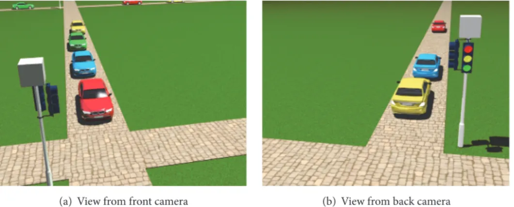
(a) View from front camera (b) View from back camera

Figure 2: In the case of the self-organizing method, if a closed-loop system (CCTV) is used, a camera for each street where vehicles enter the intersection to detect approaching vehicles is required and a camera for every street is required where vehicles exit the intersection to detect vehicle dropout. From the images acquired, an algorithm recognizes vehicles approaching and leaving the intersection.

densities, gridlocks at intersections are formed because the controller does not consider road saturation (see Figure 1). Since the green wave method does not adapt to the current traffic conditions, it is common that vehicles go slower than the green wave due to traffic density. Moreover, in realistic street networks, only two directions can be coordinated, so a considerable fraction of vehicles go against green waves, substantially increasing their waiting times.

An alternative to improve the performance of vehicular traffic is to use advanced traffic lights. The main proposed control systems using advanced traffic lights focus primarily on sensors placed at the intersection to count the vehicles approaching in certain distance [1–3]. However, the main dis-advantages that prevent the implementation of such systems are related to cost and, in some cases, privacy.

A method for controlling traffic lights using self-organization has outperformed in simulations the green wave method and has been shown to be close to optimality [4]. The essential idea of the self-organizing method is to use advanced traffic lights where sophisticated sensors detect vehicles approaching and departing from each intersection. The traffic light gives preference to the direction with

most vehicles in upstream or with most space available downstream. However, because this method also requires a sophisticated infrastructure, it has the same drawbacks of the systems mentioned previously (see Figure 2). Moreover, cameras are not suitable for detecting vehicles in visibility-limiting weather.

2. Related Work

This work focuses on vehicular traffic modeling based on cellular automata (CA). CA have an important role in the modeling of complex systems mainly because of the simplicity of their specification and the complexity in their behavior. Moreover, CA are computationally inexpensive and they can be parallelized allowing the simulation of large cities in the order of thousands of intersections. Time and space are discrete.

The behavior of vehicles on the streets can be modeled with the elementary cellular automaton (ECA) rule 184; this rule has been used to model traffic flow [9–12]. An ECA consists of a linear array of cells where the current state of each cell depends on its previous state and the current states

1 1 1 1 1 1 1 1 1 1 1 1 111 2 5 2 110 101 100 010 001 000 0 0 0 0 0 0 0 0 0 0 0 0 011 t − 1 t184 t252 t136 184 184 184 184 184 184 184 184 184 184 184 . . . . 136 2 5 2 184 184 184 184 184 184 184 184 184 184 184 136

Figure 3: Set of rules applied in the ECA city model (184, 252, and 136) and the configuration of rules around an intersection [13].

of its two closest neighbors. Each cell can take only values of 0 or 1. We can assume that one cell represents five meters, roughly the space occupied by a stationary vehicle.

Rule184 simulates traffic flow so that vehicles are repre-sented by 1 s and spaces are reprerepre-sented by 0 s. If the value of a cell is 0 and its closest neighbor to the left has value of 1, then in the next step of time the value of such a cell will change to 1. On the other hand, if the value of a cell is 1 and its closest neighbor to the left has value of 0, then in the next step of time the value of such a cell will change to 0. This models the movement of vehicles to the right. In the simulations to be presented below, streets are assumed to have only one lane in four different directions, forming a Manhattan-style grid [13]. If a light is red, all cells use rule 184 with two exceptions: rule 252 is applied to the previous cell of the intersection and rule 136 is applied to the next cell. In Figure 3, transition tables for the three rules used by the model are listed. The intersection cell is a special case, as it has four potential neighbors. The rule never changes (184). What changes is the neighborhood; that is, it takes as nearest neighbors only the two cells in the street with a green light (also using rule 184). A diagram of the cells around an intersection is shown in Figure 3.

Rule252 is used to stop traffic flow. If there is a vehicle in the central cell (i.e., 010, 011, 110, and 111), it will remain there, so that the future state of the cell will remain 1. If there is a vehicle in the previous cell (i.e., 100 and 101), the next state of the cell will be 1. Only if there are no vehicles in the previous and central cell (i.e., 000 and 001), the state of the cell will remain at 0. Rule136 is used to allow vehicles to move forward and to prevent vehicles crossing an intersection from “turning,” entering another street. Therefore, the future state of the cell will be 1 only if the cell ahead is occupied (i.e., 011 and 111).

The model of vehicular traffic proposed by Nagel and Schreckenberg [14] (NaSch) can be seen as elaboration of ECA rule 184 with the following extensions: a discrete vari-able representing the velocity associated with each vehicle, an acceleration, a deceleration (due to the presence of other vehicles), and a random tendency to slow down. This decel-eration attempts to model a human tendency to overreact while braking. The NaSch model exhibits phantom traffic

jams and, depending on both the density and the probability of slowing down, these spontaneous jams appear or disappear indefinitely. Because a vehicle can have a velocity greater than one cell per time step, the NaSch model is not an ECA. The reason is that the next state of a cell depends not only on its nearest neighbors.

Many variants of the NaSch model have been proposed, each with different degrees of realism. For example, the work presented by Nagel and Paczuski [15] inhibits the random deceleration of vehicles traveling at maximum velocity. This change eliminates phantom traffic jams and reproduces the slower-is-faster effect [16]. In the work presented by Fukui and Ishibashi [17], the authors consider only random behav-ior for vehicles traveling at maximum velocity. The random slowing of vehicles at full velocity models the fact that drivers traveling at high velocity (with no cruise control) cannot concentrate on the road indefinitely.

Cellular automaton traffic flow modeling for two dimen-sions was conceived by Biham et al. [18]. In this model (BML), each cell represents an empty space or a vehicle that is traveling to the right or up. Except for the initial random positioning of the vehicles, this automaton is deterministic. Periodic boundary conditions are considered so that the number of vehicles is preserved. On even steps, only vehicles pointing upward move, while in odd steps, only vehicles pointing right move, unless a nonempty space is in front.

The BML model is interesting for showing complex behavior (descriptive model) but not a realistic (predictive) model of vehicular traffic. More realistic vehicular traffic models have been developed as generalizations of the BML model [19–22]. Such generalizations are essentially an exten-sion BML model for which the streets have an arbitrary length (instead of a single cell) and vehicles traveling between the intersections behave according to the NaSch model. Traffic lights are incorporated into models making vehicles decelerate or stop not only because a vehicle is in front but also when approaching a red light.

Schadschneider et al. [21] experimented with a regular grid where vehicles move only right or upwards. Traffic lights were synchronized alternating between green and red (also called “marching” [23]).

In the work presented by Simon and Nagel [19], the authors developed a more elaborate combination of the BML and NaSch models. Streets with different capacities can be modeled. For example, different numbers of lanes can be considered, without explicitly simulating several lanes. For computational reasons, the computer program used random traffic lights, which have the advantage of having to be checked only when a vehicle reaches the intersection.

In relation with self-organizing traffic lights, the work presented by Gershenson and Rosenblueth [4, 5] is focused on the modeling of traffic lights to compare the perfor-mances of different control methods using elementary cel-lular automata and proposing various rules to increase the traffic flow. Two methods were evaluated to coordinate traffic lights: the traditional method called green wave and the self-organizing method. The simulations revealed the superiority of the self-organizing method over the green wave method in terms of traffic flow in a wide range of densities.

The approach by L¨ammer and Helbing [7] assumes a priority-based control of traffic lights by the vehicle flows and platoons. The considered local interactions lead to emergent coordination patterns such as green waves and achieve an efficient, decentralized traffic light control.

In the work by de Gier et al. [6], the authors compare the effects of nonadaptive versus adaptive traffic lights on generic urban road networks based on cellular automata, in which instantaneous traffic state information is sent to the traffic signal schedule. The results show that the adaptive traffic lights result in better performance compared to nonadaptive ones.

The work by Goel et al. [24] investigates the use of a distributed traffic signal control algorithm based on the concepts of self-organization. The distributed traffic signal control algorithm is benchmarked against traditional traf-fic signal algorithms. The distributed traftraf-fic signal control algorithm performs significantly better compared to the traditional traffic signal algorithms. A simulation model was created based on an abstraction of city road with multiple intersections using data on actual traffic counts.

The research by Cesme and Furth [25] explores a paradigm “self-organizing signals” for traffic signal control based on local rules that create coordination mechanisms. Simulation tests in VISSIM performed on arterial corridors in Massachusetts and Arizona show overall delay reductions.

3. Traffic Light Controllers and Measures

This section presents the green wave and self-organizing methods [4]. In addition, the measures used to evaluate the performance of the methods are described in this section. 3.1. The Green Wave Method. The idea behind the green wave method is the following: if the consecutive traffic lights switch with an offset (i.e., delay) equivalent to the expected vehicle travel time between intersections, vehicles should not have to stop. Thus, waves of green lights move through the street at the same (expected) velocity as vehicles.

This method has advantages, for example, when most of the traffic flows in the direction of the green wave at

low densities. However, vehicles flowing in the transverse direction of the green wave will be delayed. Also, if traffic is flowing at velocities lower than expected, the green waves will go faster than vehicles and there will be delays.

Implementing the green wave method in our ECA model requires synchronization of the traffic light cycle𝑇 with the travel time of the vehicles. This is achieved in our model only if the length of the street is a multiple of cycle𝑇 and periodic boundary conditions are applied. The traffic light cycle𝑇 is split into𝑇/2 for green and red light, respectively.

The lights can be in a state of a green light horizontally (east or westbound) and red light vertically (north or south-bound) or a state of a green light vertically and a red light horizontally. The state𝜎_𝑖 of the traffic lights is initialized as follows:

𝜎_𝑖 ={_{

{

green_vertical if ⌊((𝑥 − 𝑦) mod 𝑇) + 0.5⌋ ≥ 𝑇 2 green_horizontal otherwise.

(1)

Equation (1) initializes the state of a traffic light to have a green vertical light if the nearest integer of𝑥 coordinate minus𝑦 coordinate, modulus one cycle 𝑇, is greater than or equal to half a cycle. Otherwise, the state is set as horizontal green. With this equation,50% of contiguous intersections of every street (vertical and horizontal) will have a green vertical state and the other half will have a green horizontal state. The states of intersections are arranged in such a way that the transitions from horizontal green to vertical green lie on skew diagonals.

In addition, in order to set the green wave a local offset𝑤_𝑖 is necessary for each traffic light. This offset is determined by the coordinates𝑥 and 𝑦 of the intersection cells as follows:

𝑤_𝑖= ⌊((𝑥 − 𝑦) mod𝑇

2) + 0.5⌋ . (2)

Equation (2) sets the offset by rounding to the nearest integer of𝑥 coordinate minus 𝑦 coordinate, module 𝑇/2. This offset creates green waves to the south and east for regular or irregular grids. The purpose of setting the offset is to make intersections lying on the skew diagonals have the same offset value so as to switch their lights at the same time. In this way, free-flowing vehicles going either eastbound or southbound will be able to reach an intersection with a green light. To change the direction of the green wave, only the sign of𝑥 or 𝑦 coordinate has to be changed.

3.2. The Self-Organizing Method. It has been postulated that the control of the traffic lights should not be addressed as an optimization problem but as an adaptation problem because traffic flows and densities constantly change [23]. Another reason to prefer an adaptive method is that the optimiza-tion has a high computaoptimiza-tional cost to search for possible solutions, as it is an EXP-complete problem [8]. An adaptive method that applies self-organization has shown substantial improvements in increasing traffic flow at different densities compared to the green wave method [4].

r

e d

Figure 4: Rule1 attempts to turn a red light green when many vehicles approach it. Rule 2 prevents fast switching of traffic lights for high densities and also prevents a street from having always a green light. Rule3 prevents “tails” of platoons from being cut, promoting the integrity of platoons. Rule4 allows a quick change of lights at low densities, as isolated vehicles can activate the lights change as they approach an intersection without requiring them to form platoon. Rules5 and 6 prevent gridlocks caused by stationary vehicles at intersections, while allowing flow in directions with space downstream.

The essential idea of the self-organizing method is to equip traffic lights with sensors that detect approaching vehi-cles. The traffic lights give preference to the street with most vehicles. Without requiring local communication, vehicles self-organize into “platoons” which flow faster as they can trigger a green light before reaching an intersection, stopping only when another platoon is crossing.

With the self-organizing method, each intersection fol-lows independently the same rules based solely on local traffic information. There are six rules (unrelated to ECA rules), where higher-numbered rules override lower-numbered rules. The parameters to be considered in the self-organizing method and the full set of rules are shown below (see Figure 4).

The algorithm of the self-organizing method is given as follows:

(1) On every tick, add to a counter the number of vehicles approaching or waiting at a red light within distance 𝑑. When this counter exceeds a threshold 𝑛, switch the light (whenever the light switches, reset the counter to 0).

(2) Lights remain green for a minimum time 𝑢 and a maximum time𝑤.

(3) If few vehicles (𝑚 or fewer, but more than zero) are left to cross a green light at a short distance𝑟, do not switch the light.

(4) If no vehicle is approaching a green light within a distance𝑑 and at least one vehicle is approaching the red light within a distance𝑑, then switch the light. (5) If there is a stationary vehicle on the road at short

distance𝑒 beyond a green traffic light, then switch the light.

(6) If there are stationary vehicles on both directions at a short distance𝑒 beyond the intersection, then switch both lights to red. Once one of the directions is free, restore the green light in that direction.

Rules with a higher number override rules with a lower number; for example, rule 5 overrides rules 1–4. The details and rationale for all rules can be found in [5]. It should be mentioned that maximum time𝑤 was added to rule 2 in

this work, because when sensor errors occur, vehicles at low densities may remain undetected indefinitely behind a red light.

3.3. Performance Measures. The behavior of the model will depend strongly on the vehicle density𝜌 ∈ [0, 1]. Trivial cases are the extremes𝜌 = 0, where there are no vehicles, and 𝜌 = 1, where all cells are occupied by vehicles, so there is no space to move and flow is zero. The density can be easily calculated by dividing the number of cells with 1 (i.e., total number of vehicles,∑ 𝑠_𝑖) by the total number of cells (|𝑆|).

𝜌 = ∑ 𝑠𝑖

|𝑆|. (3)

The performance of the system can be measured with velocityV ∈ [0, 1], which is simply the number of cells that changed from 0 to 1 over the total number of vehicles:

V = ∑ (𝑠 󸀠 𝑖> 0)

∑ 𝑠_𝑖 , (4)

where𝑠󸀠_𝑖is the derivative of state𝑠_𝑖. If𝑠󸀠_𝑖 = 1, the cell changed from0 to 1. If 𝑠󸀠_𝑖 = −1, the cell changed from 1 to 0. 𝑠󸀠_𝑖 = 0 when there is no change in the state of𝑠_𝑖, that is, there is no vehicle, or the vehicle at𝑠_𝑖has stopped.

The flow𝐽 of the system represents how much of the space is used by moving vehicles. It can be obtained by multiplying the vehicle density by the velocity:

𝐽 = 𝜌𝜐. (5)

In the ECA rule 184 model of highway traffic, the maximum possible flow is𝐽 = 0.5 at a density 𝜌 = 0.5. This is because vehicles need at least one cell between them to move. If there are fewer vehicles, the flow will be lower, since there is no movement in free space. If there are more vehicles, then the flow will also be lower, since stationary vehicles do not move.

When coordinating traffic lights, the best performance that can be theoretically achieved would be a system in which each intersection has the best performance possible of an isolated intersection. A lower performance implies that there

Computer

Camera

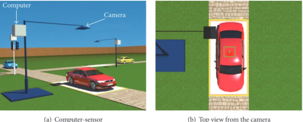
(a) Computer-sensor (b) Top view from the camera

Figure 5: The computer-sensor shown in (a) is composed of a computer and a sensor which could be a simple camera. The example illustrates possible implementation of the sensor. However, the sensor may be an inductive loop, radar, or infrared sensor. In (b), the image obtained by

computer-sensor is shown, in which only a car is recognized in the sensing area.

is interference between traffic lights. Given the properties of our model of city traffic, (6) describe the optimal curves for single intersections of velocity and flow, which depend on the maximum flow𝐽_maxallowed by an intersection:

V_optim= { { { { { { { { { { { { { { { 1 if 𝜌 ≤ 𝐽_max 𝐽max 𝜌 if 𝐽max< 𝜌 < 1 − 𝐽max 1 − 𝜌 𝜌 if 1 − 𝐽max ≤ 𝜌 𝐽_optim= { { { { { { { { { 𝜌 if 𝜌 ≤ 𝐽_max

𝐽_max if 𝐽_max< 𝜌 < 1 − 𝐽_max 1 − 𝜌 if 1 − 𝐽_max≤ 𝜌.

(6)

If𝜌 ≤ 𝐽_max, then the intersection can support a maximum velocity of 1 cells/tick. Following (5), the flow will then be equal to the density𝜌, as all vehicles are moving. If 𝐽_max< 𝜌 < 1 − 𝐽_max, then the flow of the intersection will be restricted by the maximum capacity of the intersection, that is,𝐽_max. This implies that vehicles will be using the intersection at all times, and the average velocity will be𝐽_max/𝜌. If 1 − 𝐽_max ≤ 𝜌, the density of the streets is so high that it restricts the flow of vehicles on streets, reducing the flow to1 − 𝜌 and the velocity to(1 − 𝜌)/𝜌.

Notice that the flow optimum𝐽_optimis symmetric, because there is symmetry in our city traffic model between vehicles (1 s) moving in one direction and spaces (0 s) moving in the opposite direction. This is also observed in the rule 184 model of highway traffic [12].

4. Deliberative Self-Organizing Traffic Lights

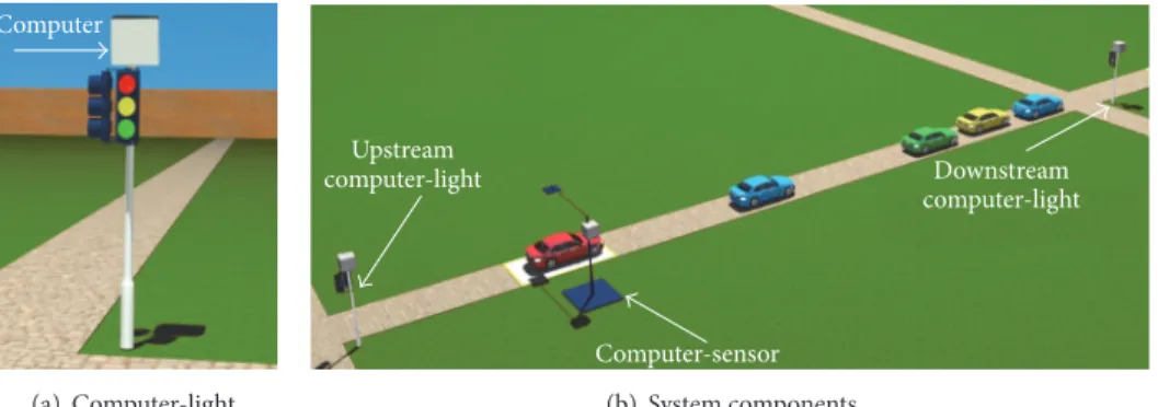
As an alternative to the limitations of the sensors required originally by the self-organizing method [5], we propose an approach using simple sensors to achieve self-organization. This involves placing at the beginning of each block a computer and a presence sensor which together are called

computer-sensor. In the same way, a computer and a traffic light are placed at each intersection which together are called computer-light.

The computer-sensor can detect only one vehicle at each time step (see Figure 5), as opposed to detecting several vehicles approaching an intersection at each time step. The computer-sensor that detects vehicles at the beginning of each block builds a virtual environment that simulates the movement of vehicles to predict which vehicles are arriving and leaving the intersection located at the end of the block (downstream). The vehicles simulated in the virtual environ-ment by the computer-sensor are called virtual vehicles.

The computer-light receives information across a data network from the computer-sensors of the neighboring blocks and runs the self-organizing method to control the traffic light.

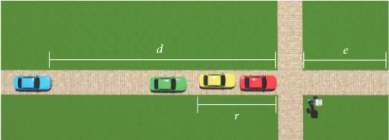
Then, for each block, the system is composed of a computer-sensor placed before the downstream intersection that sends information to the downstream computer-light (for rules 1–4) and upstream computer-light (for rules 5 and 6) (see Figure 6).

In this work, we use an ECA to simulate the virtual environment. The virtual vehicles that are at or after computer-sensor position and before the intersection are part of the set of virtual-vehicles-received by the downstream intersection. The virtual vehicles that are at or after the intersection and before the position downstream computer-sensor are part of the set of virtual-vehicles-sent (see Figure 7).

This approach compared to the current proposals using sophisticated sensors has the following advantages:

(i) The infrastructure cost is lower because the sensor and detection algorithm are less sophisticated. For example, the computer-sensor can be integrated by a Raspberry Pi and an economic camera.

(ii) Privacy is respected because the sensor is directed only to a small sensing area marked on the street. Therefore, users (pedestrians or drivers) and their routes cannot be identified.

Computer (a) Computer-light computer-light Upstream Computer-sensor Downstream computer-light (b) System components

Figure 6: The computer-sensor sends information of the positions of the virtual vehicles predicted to the downstream computer-light. The

computer-sensor also sends a message to the upstream computer-light to report if a vehicle is stationary in the sensing area. With information

from local computer-sensors, each computer-light applies the self-organizing method.

1 2 3 4 5 6 7 8 9 10 Virtual environment Virtual-vehicles-received Virtual-vehicles-sent Position of computer-sensor Position of intersection Bidirectional communication Bidirectional communication 1 1 1 1 1 1 1

Figure 7: Each sensor uses a local simulation to predict the vehicles between the sensor and the downstream

computer-light.

(iii) Vehicles do not require GPS (Global Positioning System), RFID (Radio-Frequency Identification), or other technologies to interact with the infrastructure. However, with this approach, a data network for the exchange of information is required. In the case of sophis-ticated sensors, a data network is not required, as there is no direct communication between intersections, although a network is desirable for system monitoring.

In this work, we call the self-organizing method with sophisticated sensors a reactive method because it bases its actions on current perceptions. The reactive method only maintains a counter wait time of the stationary vehicles behind a red light; however, it ignores the rest of the historical perceptions. On the other hand, we call self-organizing method with simple sensors a deliberative method because each sensor maintains an internal state that depends on the perceived history and decides whether vehicles are stationary or are approaching in the upstream and downstream inter-sections.

4.1. Deliberative Sensors Algorithm. The algorithm that runs the computer-sensor is responsible for simulating the vir-tual environment with both the information perceived by the sensor and the messages received by the downstream computer-light. The computer-sensor sends the information to the downstream computer-light to run the self-organizing traffic lights method. In addition, the computer-sensor sends information to the upstream computer-light to indirectly share this information with the computer-sensor in the upstream block. The variables used in the algorithm that runs the computer-sensor are shown in Notations.

When the computer-sensor starts its execution, it has no information on the density of vehicles that are on its block, so it assumes the worst case and completely fills the space reserved for the set of virtual-vehicles-received in the virtual environment. In addition, the computer-sensor initializes the value of variables𝑟𝑒𝑐𝑒𝑖V𝑒𝑑 and 𝑠𝑒𝑛𝑡 to zero. Subsequently, Algorithm 1 is executed at each time step.

The algorithm initializes the values of the variables𝑠𝑡𝑜𝑝 and𝑠𝑡𝑜𝑝_{𝑑𝑠𝑡𝑟𝑒𝑎𝑚}tofalse (lines (1)-(2)). If there is a vehicle in

(1) 𝑠𝑡𝑜𝑝 = 𝑓𝑎𝑙𝑠𝑒; (2) 𝑠𝑡𝑜𝑝𝑑𝑠𝑡𝑟𝑒𝑎𝑚= 𝑓𝑎𝑙𝑠𝑒 (3) V𝑒ℎ𝑖𝑐𝑙𝑒𝑠𝑡𝑎𝑡𝑒= IsThereVehicle(); (4) V𝑖𝑟𝑡𝑢𝑎𝑙_{𝑠𝑡𝑎𝑡𝑒}= isThereVirtualVehicle(); (5) if V𝑒ℎ𝑖𝑐𝑙𝑒𝑠𝑡𝑎𝑡𝑒= 𝑡𝑟𝑢𝑒 then (6) if V𝑖𝑟𝑡𝑢𝑎𝑙_{𝑠𝑡𝑎𝑡𝑒}= 𝑓𝑎𝑙𝑠𝑒 then (7) setVirtualVehicle(); (8) end if (9) V𝑒ℎ𝑖𝑐𝑙𝑒𝑠𝑡𝑜𝑝= Stationary(); (10) if V𝑒ℎ𝑖𝑐𝑙𝑒_{𝑠𝑡𝑜𝑝}= 𝑡𝑟𝑢𝑒 then (11) 𝑠𝑡𝑜𝑝 = 𝑡𝑟𝑢𝑒; (12) else (13) 𝑟𝑒𝑐𝑒𝑖V𝑒𝑑 = 𝑟𝑒𝑐𝑒𝑖V𝑒𝑑 + 1; (14) end if (15) end if (16) 𝑝𝑎𝑐𝑘𝑎𝑔𝑒₁= ReceikesMessageDownstreamCL(); (17) 𝑙𝑖𝑔ℎ𝑡𝑠𝑡𝑎𝑡𝑒= 𝑝𝑎𝑐𝑘𝑎𝑔𝑒1.𝑙𝑖𝑔ℎ𝑡𝑠𝑡𝑎𝑡𝑒; (18) 𝑠𝑡𝑜𝑝𝑑𝑠𝑡𝑟𝑒a𝑚= 𝑝𝑎𝑐𝑘𝑎𝑔𝑒1.𝑠𝑡𝑜𝑝𝑑𝑠𝑡𝑟𝑒𝑎𝑚; (19) 𝑟𝑒𝑐𝑒𝑖V𝑒𝑑_{𝑑𝑠𝑡𝑟𝑒𝑎𝑚}= 𝑝𝑎𝑐𝑘𝑎𝑔𝑒₁.𝑟𝑒𝑐𝑒𝑖V𝑒𝑑_{𝑑𝑠𝑡𝑟𝑒𝑎𝑚}; (20) 𝑟𝑒𝑠𝑢𝑙𝑡𝑠 = SimulateVirtualEnkironment(𝑙𝑖𝑔ℎ𝑡𝑠𝑡𝑎𝑡𝑒, 𝑠𝑡𝑜𝑝𝑑𝑠𝑡𝑟𝑒𝑎𝑚); (21) if 𝑟𝑒𝑠𝑢𝑙𝑡𝑠.𝑎𝑟𝑟𝑖V𝑒𝑠𝑒𝑛𝑡= 𝑡𝑟𝑢𝑒 then (22) 𝑠𝑒𝑛𝑡 = 𝑠𝑒𝑛𝑡 + 1; (23) end if (24) if 𝑟𝑒𝑠𝑢𝑙𝑡𝑠.𝑠𝑡𝑜𝑝𝑟𝑒𝑐𝑒𝑖V𝑒𝑑= 𝑡𝑟𝑢𝑒 ∧ 𝑠𝑡𝑜𝑝 = 𝑓𝑎𝑙𝑠𝑒 then (25) 𝑠𝑡𝑜𝑝 = 𝑡𝑟𝑢𝑒; (26) end if (27) if 𝑟𝑒𝑠𝑢𝑙𝑡𝑠.𝑠𝑡𝑜𝑝𝑠𝑒𝑛𝑡= 𝑡𝑟𝑢𝑒 ∧ 𝑠𝑡𝑜𝑝𝑑𝑠𝑡𝑟𝑒𝑎𝑚= 𝑓𝑎𝑙𝑠𝑒 then (28) 𝑠𝑡𝑜𝑝_{𝑑𝑠𝑡𝑟𝑒𝑎𝑚}= 𝑡𝑟𝑢𝑒; (29) end if (30) 𝑙𝑖𝑔ℎ𝑡𝑐ℎ𝑎𝑛𝑔𝑒= LightGreenChange(𝑙𝑖𝑔ℎ𝑡𝑠𝑡𝑎𝑡𝑒); (31) if 𝑙𝑖𝑔ℎ𝑡_{𝑐ℎ𝑎𝑛𝑔𝑒}= 𝑡𝑟𝑢𝑒 then (32) 𝜖 = |𝑟𝑒𝑐𝑒𝑖V𝑒𝑑𝑑𝑠𝑡𝑟𝑒𝑎𝑚− 𝑠𝑒𝑛𝑡|; (33) 𝑠𝑒𝑛𝑡 = 0; (34) end if (35) 𝑟𝑒𝑠𝑢𝑙𝑡𝑠 = CountVehiclesVirtualEnkironment(); (36) 𝑝𝑎𝑐𝑘𝑎𝑔𝑒2.𝑛 = 𝑟𝑒𝑠𝑢𝑙𝑡𝑠.𝑛 + 𝜖 (37) 𝑝𝑎𝑐𝑘𝑎𝑔𝑒₂.𝑚 = 𝑟𝑒𝑠𝑢𝑙𝑡𝑠.𝑚 (38) 𝑝𝑎𝑐𝑘𝑎𝑔𝑒2.𝑠𝑡𝑜𝑝 = 𝑠𝑡𝑜𝑝𝑑𝑠𝑡𝑟𝑒𝑎𝑚 (39) SendMessageDownstreamCL(𝑝𝑎𝑐𝑘𝑎𝑔𝑒2); (40) 𝑝𝑎𝑐𝑘𝑎𝑔𝑒₃.𝑠𝑡𝑜𝑝 = 𝑠𝑡𝑜𝑝 (41) 𝑝𝑎𝑐𝑘𝑎𝑔𝑒₃.𝑟𝑒𝑐𝑒𝑖V𝑒𝑑 = 𝑟𝑒𝑐𝑒𝑖V𝑒𝑑 (42) SendMessageUpstreamCL(𝑝𝑎𝑐𝑘𝑎𝑔𝑒3); (43) 𝑝𝑎𝑐𝑘𝑎𝑔𝑒₄= ReceikesMessageUpstreamCL(); (44) if 𝑝𝑎𝑐𝑘𝑎𝑔𝑒₄.𝑙𝑖𝑔ℎ𝑡_{𝑐ℎ𝑎𝑛𝑔𝑒}= 𝑡𝑟𝑢𝑒 then (45) 𝑟𝑒𝑐𝑒𝑖V𝑒𝑑 = 0; (46) end if

Algorithm 1: Deliberative sensors algorithm.

the sensing area, the function IsThereVehicle returnstrue when such a condition is satisfied and false otherwise (line (3)). If there is a virtual vehicle in the position of the sensing area of the virtual environment, the function

isThereVirtualVehiclereturnstrue when such a condition

is satisfied and false otherwise (line (4)). If a vehicle is sensed and the virtual vehicle is not registered in the corre-sponding position of the virtual environment, the function

setVirtualVehicle creates a virtual vehicle in that position

(line (7)). The verification is done to prevent the removal of a virtual vehicle and add it again in the same position. A case often occurs when a stationary vehicle in the sensing area is already registered in that position of the virtual environment. The function Stationary checks if there is a stationary vehicle in the sensing area. If such a condition istrue, it returnstrue and false otherwise (line (9)). If the vehicle is stationary, the variable 𝑠𝑡𝑜𝑝 is set to true to indicate a stationary vehicle in the sensing area at the beginning of

the block. Otherwise, if the vehicle is moving, the variable 𝑟𝑒𝑐𝑒𝑖V𝑒𝑑 is increased by one to indicate that a vehicle is received in the sensing area (line (13)).

The computer-sensor through the function

ReceivesMes-sageDownstreamCL receives a package from the

down-stream computer-light. The package contains information regarding the status of the traffic light, whether a vehicle is stationary, and the number of vehicles received in the downstream block. Subsequently, the information is set to the variables 𝑙𝑖𝑔ℎ𝑡_{𝑠𝑡𝑎𝑡𝑒}, 𝑠𝑡𝑜𝑝_{𝑑𝑠𝑡𝑟𝑒𝑎𝑚}, and 𝑟𝑒𝑐𝑒𝑖V𝑒𝑑_{𝑑𝑠𝑡𝑟𝑒𝑎𝑚}, respectively (lines (17)–(19)).

The function SimulateVirtualEnvironment simulates in the virtual environment the movement of the vehicles (line (20)):

(i) The movement of each member of the set of virtual-vehicles-received is simulated depending on the value of the variable 𝑙𝑖𝑔ℎ𝑡_{𝑠𝑡𝑎𝑡𝑒} (red or green) and the position of neighboring virtual vehicles. If a virtual vehicle received goes through a green light and is at or after the intersection, it becomes part of the set of virtual-vehicles-sent.

(ii) The movement of each member of the set of virtual-vehicles-sent is simulated depending on the state vari-able𝑠𝑡𝑜𝑝_{𝑑𝑠𝑡𝑟𝑒𝑎𝑚}(true or false) and the position of neighboring virtual vehicles. The variable𝑠𝑡𝑜𝑝_{𝑑𝑠𝑡𝑟𝑒𝑎𝑚} is similar to the traffic lights; if𝑠𝑡𝑜𝑝_{𝑑𝑠𝑡𝑟𝑒𝑎𝑚} is true and there are virtual vehicles in the set of virtual-vehicles-sent, the virtual vehicles cannot advance. If a virtual vehicle reaches the position of the down-stream computer-sensor, the virtual vehicle is removed from the set of virtual-vehicles-sent and the function

SimulateVirtualEnvironmentreturns a value in the

package 𝑟𝑒𝑠𝑢𝑙𝑡𝑠 to indicate that a virtual vehicle arrived (line (20)).

If the simulation registers a virtual vehicle that reaches the downstream computer-sensor on the set of virtual-vehicles-sent, the computer-sensor increases the value of the variable 𝑠𝑒𝑛𝑡 by one (lines (21)–(23)).

If the simulation registers a virtual stationary vehicle in the sensing area and the variable𝑠𝑡𝑜𝑝 has the value false, then the value of the variable𝑠𝑡𝑜𝑝 is set in true because the computer-sensor chooses the possibility that an error sensing occurred (lines (24)–(26)).

If the virtual simulation registers a virtual stationary vehicle on the set of virtual-vehicles-sent and the variable 𝑠𝑡𝑜𝑝_{𝑑𝑠𝑡𝑟𝑒𝑎𝑚} has the value false, then the value of the variable 𝑠𝑡𝑜𝑝_{𝑑𝑠𝑡𝑟𝑒𝑎𝑚} is set in true because the computer-sensor selects the possibility that a sensing error occurred in the downstream computer-sensor to avoid traffic jams at the intersection (lines (27)–(29)).

It should be mentioned that because the overall simu-lation runs on an ECA, the virtual environment that runs the computer-sensor is performed with a local ECA, and considering a perfect sensor, intuitively it is natural to think that the simulation is completely deterministic. However, this is not the case because of the following reasons:

(i) At the beginning of the simulation, the computer-sensor has no information so it assumes the worst case and considers that the set of virtual-vehicles-received is full. In addition, the computer-sensor assumes that no virtual vehicle has been sent. Therefore, the “real” traffic state does not correspond to the state of the local virtual environment of the computer-sensor and the algorithm must implement a mechanism to rectify the situation.

(ii) When a computer-sensor receives a green light, it assumes that the vehicles have started moving. How-ever, in the global simulation, if a vehicle has a green light but there is another vehicle in the transversal direction occupying the intersection, then the vehicle does not advance and the prediction in the virtual environment will be out of phase. Thus, the algorithm should also rectify this situation.

(iii) The sensors may have errors, and consequently some vehicles may not be detected.

The function GreenLightChange determines if the light of the downstream traffic light turned green and when the condition is true the absolute difference between the number of vehicles received by the downstream block and the number of virtual vehicles sent is calculated. Such a difference is set to the variable𝜖 (line (32)). If the numbers of vehicles in 𝑟𝑒𝑐𝑒𝑖V𝑒𝑑_{𝑑𝑠𝑡𝑟𝑒𝑎𝑚} and number of virtual vehicles sent are equal, then the value of the variable𝜖 is set to zero because the numbers predicted between vehicles received by the downstream computer-sensor and virtual vehicles sent by the computer-sensor match. On the other hand, prediction errors occur if the numbers of vehicles received and the virtual

vehicles sent do not match, the value of𝜖 is nonzero, and the

value of the variable𝑠𝑒𝑛𝑡 is set to zero (lines (32)-(33)). The function CountVehiclesVirtualEnvironment counts the number of virtual vehicles that are received at distance𝑑 and distance𝑟 from the position of the intersection and set to variables𝑛 and 𝑚 of the data structure 𝑟𝑒𝑠𝑢𝑙𝑡𝑠. The data structure𝑟𝑒𝑠𝑢𝑙𝑡𝑠 is the value returned by the function (line (35)). Subsequently, a package is created with the data𝑛 set to 𝑛 + 𝜖, 𝑚 set to 𝑚, and 𝑠𝑡𝑜𝑝 set to 𝑠𝑡𝑜𝑝𝑑𝑠𝑡𝑟𝑒𝑎𝑚(lines (36)–(38)). The package is sent by the function

SendMessageDown-streamCL to downstream computer-light (line (39)). The

downstream computer-light with the information contained in the package applies the method of self-organizing traffic lights.

The number of virtual vehicles received at distance𝑑 and distance𝑟 is increased with 𝜖 to adjust the gap between the number of vehicles received by the downstream block and virtual vehicles sent. The increase in the number of virtual vehicles received gives priority to the block for mitigating two undesirable situations:(1) when the number of virtual vehicles sent is lower than the vehicles received, it is inferred that the missing vehicles are still in the previous block;(2) when the number of virtual vehicles sent is greater than the vehicles received, it is inferred that there are excess vehicles in the previous block.

The computer-sensor through the function

0.8 1.0 0.6 0.2 0.4 0.0 Density 0.00 0.05 0.10 0.15 0.20 0.25 0.30 Flo w Green wave Self-organizing reactive Self-organizing deliberative Optimality curve (a) Flow 0.8 1.0 0.6 0.2 0.4 0.0 Density 0.0 0.2 0.4 0.6 0.8 1.0 Ve lo ci ty Green wave Self-organizing reactive Self-organizing deliberative Optimality curve (b) Velocity

Figure 8: The reactive and deliberative self-organizing methods achieve good performance for all densities compared to the green wave method. Both self-organizing methods are close to the optimality curves (see (6)).

variables𝑠𝑡𝑜𝑝 and 𝑟𝑒𝑐𝑒𝑖V𝑒𝑑 to the upstream computer-light (lines (40)–(42)). The package contains information regard-ing whether a vehicle is stationary and the number of vehicles received on the block of computer-sensor.

Finally, the computer-sensor through the function

ReceivesMessageUpstreamCL receives a package of

upstream computer-light to report that the light of the upstream traffic light turned green and set the value of the variable𝑟𝑒𝑐𝑒𝑖V𝑒𝑑 to zero (lines (43)–(46)).

A system in the city of Duisburg has been developed with the purpose of predicting the state of the traffic by online simulation of virtual vehicles with cellular automata [26, 27]. Like our approach with deliberative traffic lights, in the Duis-burg system, it is necessary to place sensors (inductive cycles) on the roads to detect the presence of the vehicles. However, unlike deliberative traffic lights, the Duisburg system has a centralized approach because one computer collects all the information obtained by the sensors and another computer executes the simulation on a global level. Our approach with deliberative traffic lights, by contrast, is distributed because each computer-sensor collects the information and simulates the corresponding traffic only in its block, that is, at the local level. Deliberative traffic lights have the advantage that if a computer-sensor fails, it does not imply that the entire system collapses, which does occur in the Duisburg system when the computer that collects the information from the sensors or the computer that performs the simulation fails.

In addition, the online simulation of the Duisburg system aims to plan routes according to the state of the predicted traffic which will be sent to the driver. On the other hand, with the deliberative traffic lights, the simulation of each computer-sensor has the objective of managing the traffic light.

5. Results

To test the green wave and the reactive and deliberative self-organizing traffic lights methods, we constructed a hundred-by-hundred homogeneous street grid with alternating flow directions and cyclic boundaries. In our green wave method, the cycle𝑇 = 85. The length of each street is 1,700 cells, that is, 8,500 meters (each cell is five meters). Every block has a distance of 16 cells (without the intersection). Thus, there are 80 simulated meters between streets (similar to streets in Manhattan). In the grid there are 330,000 cells, 10,000 intersections, and 200 streets (50 in each cardinal direction). It is worth mentioning that Manhattan has approximately 3,360 intersections, so the simulated city is about three times the size of Manhattan.

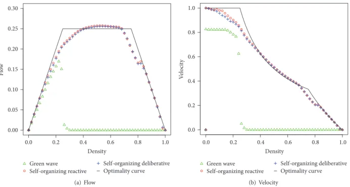
The experiments consist in running the simulation with 50 different densities for the green- and the reactive and deliberative self-organizing methods. For each density, ten runs were executed and the results were averaged. Each run consisted of the following: there is an initial state where vehicles are placed randomly and homogeneously. Then, half an hour (5,400 ticks) is simulated. After these initial 5,400 ticks, the system is considered to have stabilized, that is, gone through a transient, so another half hour is simulated, where the velocity is measured at every tick. At the end of the simulation, the velocities of the second half hour are averaged to obtain the average velocityV and average flow 𝐽. The results are shown in Figure 8.

Table 1 shows the values of the parameters used by the self-organizing methods, as proposed in [4].

The simulator with which we performed our experiments was developed in the C language. The reader is invited

Table 1: Parameters used by the self-organizing method [4]. The size of each block is80 meters. Variable Abstract value Scaled value Description

Δ𝑡 1 tick 1/3 s Time step in the simulation.

𝑑 10 cells 50 m Distance where the vehicles are detected approaching the intersection. 𝑟 5 cells 25 m Short distance where the vehicles are detected approaching the intersection. 𝑒 3 cells 15 m Distance where stationary vehicles are detected.

𝑢 10 ticks 3.33 s Minimum waiting time behind a red light. 𝑤 600 ticks 200 s Maximum waiting time behind a red light. 𝑛 40 veh⋅ticks 13.33 veh⋅s Accumulated number of vehicles at distance𝑑. 𝑚 2 vehicles 2 vehicles Number of vehicles at distance𝑟.

to access the code at https://github.com/Zapotecatl/Traffic-Light.

In the green wave method, we found the following phases: (i) The intermittent phase is between𝜌 > 0 and 𝜌 ⪅ 0.22. At this phase, some vehicles are stationary behind a red light. The phase transition lies at𝜌 ≈ 0.22, where there is a maximum flow of𝐽≈ 0.17 (see Figure 8). (ii) The gridlock phase is presented for densities 𝜌 ⪆

0.22; vehicles flowing on streets with green wave (southbound and eastbound) cannot keep the velocity of the green wave, so traffic jams move in the opposite direction of the flow. The queues of vehicles and platoons groups waiting behind a red light grow in opposite directions of the green wave and block intersections. Consequently, gridlocks occur (see Fig-ure 8).

For the reactive and deliberative self-organizing methods, we found the following phases:

(i) The free-flow phase is presented only for very low den-sities in the reactive and deliberative self-organizing methods in0 < 𝜌 ⪅ 0.000006, where V = 1 and no vehicle has to stop. It should be noted that this phase almost disappeared because of the introduction of a maximum time𝑤 in rule 2. Nevertheless, this phase does not exist in realistic scenarios, as it requires periodic boundaries and no turning vehicles. (ii) The quasi-free-flow phase is presented in the

reac-tive and deliberareac-tive self-organizing method in 0.000006 < 𝜌 ⪅ 0.12, where few vehicles stop for little time. Most intersections have only one platoon requesting a green light, so this one is able to flow without having to stop, unless another platoon is crossing at the same time.

(iii) The intermittent underutilized phase is presented in the reactive and deliberative self-organizing method between𝜌 ≈ 0.12 and 𝜌 ≈ 0.22, where intersections are idling some of the time; that is, no vehicle uses them. The difference with the quasi-free-flow phase is that in the underutilized intermittent phase there are two platoons requesting a green light in most of the cases. Thus, one platoon has to wait until the other one crosses.

(iv) The quasi-full capacity intermittent phase is presented in the reactive and deliberative self-organizing meth-ods between 𝜌 ≈ 0.22 and 𝜌 ≈ 0.4. There are always two platoons requesting a green light; however, there is a certain probability that the platoons are of different sizes. The smallest platoons generate lower demand and lead to idle intersections.

(v) The full capacity intermittent phase is presented in the reactive and deliberative self-organizing method between𝜌 ≈ 0.4 and 𝜌 ≈ 0.68 with a maximum flow𝐽≈ 0.257. This implies that the intersections are being used at full capacity. In the full capacity intermittent phase there are no resources “lost” of free space because the intersections are being used constantly; that is, there are always vehicles crossing all intersections.

(vi) The overutilized intermittent phase is presented in the reactive and deliberative self-organizing methods between𝜌 ≈ 0.68 and 𝜌 ≈ 0.8, where the density is such that rule6 sometimes forces both directions to stop, thus reducing the flow of the intersections. This phase is similar to the underutilized intermittent phase in the sense that the intersections cannot be used at their full flow capacity. In the underutilized intermittent case, this is because there are no enough vehicles. In the overutilized intermittent case, by contrast, this is because there are too many vehicles and intersections need to wait before one street can get a green light.

(vii) The quasi-gridlock phase is presented in the reactive and deliberative self-organizing methods between 𝜌 ≈ 0.8 and 𝜌 < 1.0. Most vehicles are stationary, but free spaces move in the direction opposite of the vehicles between traffic jams at a velocity of one cell per tick.

(viii) The gridlock phase is presented for high densities in the reactive and deliberative self-organizing method in𝜌 = 1.0; that is, V = 0. The vehicles cannot move because the density is too high and intersections are blocked from initial conditions.

5.1. Errors on Sensors. Each sensor has associated a proba-bility𝑃 that represents the precision to detect vehicles, for example, if𝑃 = 0.9 sensor will detect 90% of vehicles. This

0.8 1.0 0.6 0.2 0.4 0.0 Density 0.00 0.05 0.10 0.15 0.20 0.25 0.30 Flo w P = 80% P = 90% P = 100% P = 50% P = 60% P = 70%

(a) Reactive self-organizing

0.8 1.0 0.6 0.2 0.4 0.0 Density 0.00 0.05 0.10 0.15 0.20 0.25 0.30 Flo w P = 80% P = 90% P = 100% P = 50% P = 60% P = 70% (b) Deliberative self-organizing

Figure 9: Flow-density diagrams for different error rates.𝑃 represents the accuracy of the sensor.

probability of precision is implemented within the function

IsThereVehicle. Therefore, in the reactive self-organizing

method, the function IsThereVehicle is called to verify the𝑘 cells contained within the sensing zone between the distances 𝑑 and 𝑒. Moreover, in the case of deliberative self-organizing method, the function IsThereVehicle is called once because the sensing area is only formed by a cell. In addition, at the time a vehicle is no longer detected by the sensor, the vehicle will remain imperceptible throughout its entire trajectory in the sensing area.

The experiment consists in executing the simulation with six different degrees of sensor precision𝑃, 1.0, 0.9, 0.8, 0.7, 0.6, and 0.5, to evaluate the robustness of reactive and deliberative self-organizing methods against errors sensing.

The configuration used for each run is the same as the experiments of the previous section to evaluate the performance of the three methods to control traffic lights. The results of the self-organizing reactive approach compared to the self-organizing deliberative method are shown in Figure 9.

The simulation results with sensors to different levels of precision show that the deliberative self-organizing approach is more robust to sensing errors. This is because the delib-erative method maintains the state of the environment in memory and sensing error only affects a cell. On the other hand, in the traditional approach, the state of the system is not maintained and the error is distributed in all cells because it is inherent in the sensing area. Therefore, the reactive method has no way to recover and requires a high degree of precision of the sensor because even when the precision of sensor is 90%, the flow collapses.

6. Discussion

In our green wave method, the cycle𝑇 controls the synchro-nization of the traffic light with the travel time of vehicles around the torus. This synchronization is achieved in our model if the street length is a multiple of𝑇, a condition for free-flow. Otherwise, the cycle of the traffic light and the travel time of the vehicles are out of synchrony. Thus, vehicles need to wait for a green light and the average velocity is less than one. We contrast the green wave method using the same settings in section 5 (Results) applying a global cycle𝑇 = 85 with the green wave method applying a local cycle𝑇_𝑖at each traffic light set in a random value in the range of[2, 𝑇]. The lower limit of the range is 2 so as to give at least one time step for the green light and one time step for the red light. When the value of𝑇 is not the same for all traffic lights, there is no coordination between traffic lights and the flow is reduced because the movement of the vehicles is interfered by red lights (see Figure 10).

Our deliberative self-organizing algorithm bases its per-formance on the precision of the computer-sensor to detect and predict the movement of the vehicles in its block. However, if our ACE model allows vehicles to turn, the computer-sensor receives information from another block, a situation for which the deliberative self-organizing algorithm is not designed. In addition, when a vehicle tries to turn to enter a transverse street that is saturated, the flow stops because the vehicle obstructs the intersection and there is only one lane. The flow is not released until there is a space in the street where the vehicle is trying to enter or the vehicle decides to continue in the same direction in which it was.

0.8 1.0 0.6 0.2 0.4 0.0 Density 0.00 0.05 0.10 0.15 0.20 0.25 0.30 Flo w

Green wave, global T = 85 Green wave, global Ti = [2, T]

(a) Flow 0.8 1.0 0.6 0.2 0.4 0.0 Density 0.0 0.2 0.4 0.6 0.8 1.0 Ve lo ci ty

Green wave, global T = 85 Green wave, global Ti = [2, T]

(b) Velocity

Figure 10: Flow-density and velocity-density diagrams for green wave with the same global cycle𝑇 and a local cycle in the range of [2, 𝑇].

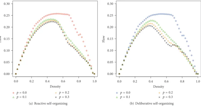
0.8 1.0 0.6 0.2 0.4 0.0 Density 0.00 0.05 0.10 0.15 0.20 0.25 0.30 Flo w p = 0.0 p = 0.1 p = 0.3 p = 0.2

(a) Reactive self-organizing

0.8 1.0 0.6 0.2 0.4 0.0 Density 0.00 0.05 0.10 0.15 0.20 0.25 0.30 Flo w p = 0.0 p = 0.1 p = 0.3 p = 0.2 (b) Deliberative self-organizing

Figure 11: Flow-density and velocity-density diagrams for different probabilities of turn in the reactive and deliberative algorithm.

Approximately 20% of the vehicles turn into important avenues. However, the percentage is different depending on the topology of each city. In order to explore the effects produced in the reactive and deliberative self-organizing algorithm with the previously mentioned situations, we did an experiment consisting in varying the probability that a vehicle decides to turn at an intersection at 𝑝 = {0.0, 0.1, 0.2, 0.3} (see Figure 11). The case with 𝑝 = 0 is

relevant for its quasi symmetry and for the identification of phase transitions. A greater probability will cause more vehicles to attempt to enter other transversal streets, but there will also be a greater probability that such vehicles will again decide to change direction and continue their travel in the direction in which they were.

Figure 11 shows that the flow decreases in the deliberative and reactive self-organizing algorithm when vehicles turn.

When the density is increased, the possibility that a vehicle tries to enter a transverse street that is saturated is greater and therefore the flow is reduced.

Although our deliberative self-organizing algorithm was designed with the restriction that vehicles can only go in one direction, when vehicles are allowed to turn, the algorithm shows a similar performance to that of the reactive self-organizing algorithm. A future extension to our deliberative self-organizing algorithm is to delegate to the computer-light the responsibility of applying or not applying the compen-sation (through epsilon) to mitigate the prediction errors. For example, if an intersection has horizontal downstream computer-light with a missing vehicle but in the vertical downstream computer-light there is a surplus vehicle, the computer-light infers that a vehicle turns and would not apply compensations.

Our experiments with errors on sensors show that a convenient strategy when sensors fail more than 10% is that the traffic lights apply the green wave method because it has a better performance in that case.

7. Conclusions

All major cities suffer from traffic jams. Technological improvements such as the one presented here can increase the capacity of urban infrastructure. However, if it becomes very efficient to travel by private vehicle, more people will be inclined to do so, increasing density and eventually decreasing traffic flow. This means that improvements to traffic infrastructure can actually generate a worse situation than the one they are trying to solve [28, 29]. For this reason, an integrated transportation plan is required to balance the demands and improvements over all transportation modes.

Our city traffic model [13] is more useful for descriptive than predictive purposes. Its vehicle-space duality (both occupy the same space) yields symmetry in the flow opti-mality curves. Its simplicity allows the clear identification of phase transitions. We have also worked with realistic city traffic models [30, 31], obtaining similar results. We are in the process of developing a more realistic city traffic model to bridge both lines of research.

It is clear that adaptive algorithms will outperform tra-ditional static methods [32], as it was shown here. It is also important to develop robust methods, and the deliberative sensors achieve a considerable improvement over sophisti-cated sensors. In the performed experiments, 30% failure rate of the deliberative sensors performed better than 10% failure rate with sophisticated sensors.

Sophisticated sensors could be improved to increase their robustness, for example, adding more cameras or processing, but this would increase their cost even more. As sensor technology evolves, probably it will be common to deploy robust and cheap sensors in cities in the near future. There might be other ways to increase the robustness of this approach, but its exploration is beyond the scope of this work. Considering the recent progress made in the development of autonomous vehicles [33, 34], decentralized algorithms such as the ones presented here will be useful in the coor-dination of autonomous vehicles at intersections as well.

Notations

𝑙𝑖𝑔ℎ𝑡𝑠𝑡𝑎𝑡𝑒: If the value is set totrue, the traffic light is green. Otherwise, the light is red 𝑠𝑒𝑛𝑡: Number of vehicles sent to the

downstream block

𝑟𝑒𝑐𝑒𝑖V𝑒𝑑: Number of vehicles received

𝑠𝑡𝑜𝑝: If the value is set totrue, a stationary vehicle is in the sensing area

𝑟𝑒𝑐𝑒𝑖V𝑒𝑑_{𝑑𝑠𝑡𝑟𝑒𝑎𝑚}: Number of vehicles received in the downstream block

𝑠𝑡𝑜𝑝_{𝑑𝑠𝑡𝑟𝑒𝑎𝑚}: If the value is set totrue, there is a stationary vehicle in the sensing area of downstream block

𝜖: Absolute difference between the number of vehicles received and virtual vehicles sent on the downstream block.

Conflicts of Interest

The authors declare that there are no conflicts of interest regarding the publication of this paper.

Acknowledgments

The authors gratefully acknowledge the facilities provided by Department of Computer Science, Instituto de Investiga-ciones en Matem´aticas Aplicadas y en Sistemas at Universi-dad Nacional Aut´onoma de M´exico. Jorge L. Zapotecatl was supported by the scholarship 380281 of CONACyT, M´exico. The authors acknowledge support from CONACyT Grants 221341 and 212802.

References

[1] R. A. Vincent and C. P. Young, “Self optimising traffic signal control using microprocessors—the TRRL MOVA strategy for isolated intersections,” Traffic Engineering and Control, vol. 27, no. 7-8, pp. 385–387, 1986.

[2] P. Mirchandani and L. Head, “A real-time traffic signal control system: architecture, algorithms, and analysis,” Transportation

Research Part C: Emerging Technologies, vol. 9, no. 6, pp. 415–

432, 2001.

[3] S. F. Smith, G. J. Barlow, X. F. Xie, and Z. B. Rubinstein, “Smart urban signal networks: initial application of the SURTRAC adaptive traffic signal control system,” in Proceedings of the 23rd

International Conference on Automated Planning and Scheduling (ICAPS ’13), June 2013.

[4] C. Gershenson and D. A. Rosenblueth, “Adaptive self-organization vs static optimization: a qualitative comparison in traffic light coordination,” Kybernetes, vol. 41, no. 3, pp. 386–403, 2012.

[5] C. Gershenson and D. A. Rosenblueth, “Self-organizing traffic lights at multiple-street intersections,” Complexity, vol. 17, no. 4, pp. 23–39, 2012.

[6] J. de Gier, T. M. Garoni, and O. Rojas, “Traffic flow on realistic road networks with adaptive traffic lights,” Journal of Statistical

Mechanics, vol. 2011, no. 4, Article ID P04008, 2011.

[7] S. L¨ammer and D. Helbing, “Self-control of traffic lights and vehicle flows in urban road networks,” Journal of

Statisti-cal Mechanics: Theory and Experiment, vol. 2008, Article ID

[8] J. T¨or¨ok and J. Kert´esz, “The green wave model of two-dimensional traffic: transitions in the flow properties and in the geometry of the traffic jam,” Physica A: Statistical Mechanics and

Its Applications, vol. 231, no. 4, pp. 515–533, 1996.

[9] S. Yukawa, M. Kikuchi, and S.-I. Tadaki, “Dynamical phase transition in one dimensional traffic flow model with blockage,”

Journal of the Physical Society of Japan, vol. 63, no. 10, pp. 3609–

3618, 1994.

[10] D. Chowdhury, L. Santen, and A. Schadschneider, “Statistical physics of vehicular traffic and some related systems,” Physics

Reports. A Review Section of Physics Letters, vol. 329, no. 4–6,

pp. 199–329, 2000.

[11] S. Maerivoet and B. De Moor, “Cellular automata models of road traffic,” Physics Reports. A Review Section of Physics Letters, vol. 419, no. 1, pp. 1–64, 2005.

[12] M. Kanai, “Calibration of the particle density in cellular-automaton models for traffic flow,” Journal of the Physical Society

of Japan, vol. 79, no. 7, Article ID 075002, 2010.

[13] D. A. Rosenblueth and C. Gershenson, “A model of city traffic based on elementary cellular automata,” Complex Systems, vol. 19, no. 4, pp. 305–322, 2011.

[14] K. Nagel and M. Schreckenberg, “A cellular automaton model for freeway traffic,” Journal of Physics I France, vol. 2, no. 12, pp. 2221–2229, 1992.

[15] K. Nagel and M. Paczuski, “Emergent traffic jams,” Physical

Review E, vol. 51, no. 4, pp. 2909–2918, 1995.

[16] C. Gershenson and D. Helbing, “When slower is faster,”

Com-plexity, vol. 21, no. 2, pp. 9–15, 2015.

[17] M. Fukui and Y. Ishibashi, “Traffic flow in 1d cellular automaton model including cars moving with high speed,” Journal of the

Physical Society of Japan, vol. 65, no. 6, pp. 1868–1870, 1996.

[18] O. Biham, A. A. Middleton, and D. Levine, “Self-organization and a dynamical transition in traffic-flow models,” Physical

Review A, vol. 46, no. 10, pp. R6124–R6127, 1992.

[19] P. M. Simon and K. Nagel, “A simplified cellular automaton model for city traffic,” Tech. Rep. LA-UR 97-707, LANL, 1997. [20] D. Chowdhury and A. Schadschneider, “Self-organization of

traffic jams in cities: effects of stochastic dynamics and signal periods,” Physical Review E, vol. 59, no. 2, pp. R1311–R1314, 1999. [21] A. Schadschneider, D. Chowdhury, E. Brockfeld, K. Klauck, L. Santen, and J. Zittartz, “A new cellular automata model for city traffic,” in Proceedings of the Traffic and Granular Flow ’99:

Social, Traffic, and Granular Dynamics, Springer, 1999.

[22] E. Brockfeld, R. Barlovic, A. Schadschneider, and M. Schreck-enberg, “Optimizing traffic lights in a cellular automaton model for city traffic,” Physical Review E, vol. 64, no. 5, Article ID 056132, 12 pages, 2001.

[23] C. Gershenson, “Self-organizing traffic lights,” Complex

Sys-tems, vol. 16, no. 1, pp. 29–53, 2005.

[24] S. Goel, S. F. Bush, and K. Ravindranathan, “Self-organization of traffic lights for minimizing vehicle delay,” in Proceedings of

the 3rd International Conference on Connected Vehicles and Expo (ICCVE ’14), pp. 931–936, aut, November 2014.

[25] B. Cesme and P. G. Furth, “Self-organizing traffic signals using secondary extension and dynamic coordination,”

Transporta-tion Research Part C: Emerging Technologies, vol. 48, pp. 1–15,

2014.

[26] J. Wahle, J. Esser, L. Neubert, and M. Schreckenberg, A Cellular

Automaton Traffic Flow Model for Online-Simulation of Urban Traffic, Springer, London, UK, 1998.

[27] J. Wahle, L. Neubert, J. Esser, and M. Schreckenberg, “A cellular automaton traffic flow model for online simulation of traffic,”

Parallel Computing, vol. 27, no. 5, pp. 719–735, 2001.

[28] D. Braess, A. Nagurney, and T. Wakolbinger, “On a paradox of traffic planning,” Transportation Science, vol. 39, no. 4, pp. 446– 450, 2005.

[29] R. Steinberg and W. I. Zangwill, “The prevalence of Braess’ paradox,” Transportation Science, vol. 17, no. 3, pp. 301–318, 1983. [30] S. B. Cools, C. Gershenson, and B. D’Hooghe, “Self-organizing traffic lights: a realistic simulation,” in Self-Organization:

Applied Multi-Agent Systems, M. Prokopenko, Ed., pp. 41–49,

Springer, 2007.

[31] D. Zubillaga, G. Cruz, L. D. Aguilar et al., “Measuring the complexity of self-organizing traffic lights,” Entropy, vol. 16, no. 5, pp. 2384–2407, 2014.

[32] C. Gershenson, “Living in living cities,” Artificial Life, vol. 19, no. 3-4, pp. 401–420, 2013.

[33] R. Bishop, “A survey of intelligent vehicle applications world-wide,” in Proceedings of the Intelligent Vehicles Symposium IV ’20, pp. 25–30, IEEE, 2000.

[34] R. Tachet, P. Santi, S. Sobolevsky et al., “Revisiting Street Intersections Using Slot-Based Systems,” PLoS ONE, vol. 11, no. 3, pp. 1–9, 2016.