Evaluation of two ozone air quality modelling systems

(1)

HAL Id: hal-00301173

https://hal.archives-ouvertes.fr/hal-00301173

Submitted on 24 Mar 2004

HAL is a multi-disciplinary open access

archive for the deposit and dissemination of sci-entific research documents, whether they are pub-lished or not. The documents may come from teaching and research institutions in France or abroad, or from public or private research centers.

L’archive ouverte pluridisciplinaire HAL, est destinée au dépôt et à la diffusion de documents scientifiques de niveau recherche, publiés ou non, émanant des établissements d’enseignement et de recherche français ou étrangers, des laboratoires publics ou privés.

Evaluation of two ozone air quality modelling systems

S. Ortega, M. R. Soler, J. Beneito, D. Pino

To cite this version:

S. Ortega, M. R. Soler, J. Beneito, D. Pino. Evaluation of two ozone air quality modelling systems. Atmospheric Chemistry and Physics Discussions, European Geosciences Union, 2004, 4 (2), pp.1855-1885. �hal-00301173�

(2)

ACPD

4, 1855–1885, 2004

Evaluation of two ozone air quality modelling systems S. Ortega et al. Title Page Abstract Introduction Conclusions References Tables Figures J I J I Back Close Full Screen / Esc

Print Version Interactive Discussion

Atmos. Chem. Phys. Discuss., 4, 1855–1885, 2004 www.atmos-chem-phys.org/acpd/4/1855/

SRef-ID: 1680-7375/acpd/2004-4-1855 © European Geosciences Union 2004

Atmospheric Chemistry and Physics Discussions

Evaluation of two ozone air quality

modelling systems

S. Ortega1, M. R. Soler1, J. Beneito1, and D. Pino2, 3

1

Department of Astronomy and Meteorology, University of Barcelona, Avd. Diagonal 647, 08028 Barcelona, Spain

2

Institute for Space Studies of Catalonia, Edifici Nexus 2, Gran Capit `a 2–4, 08034 Barcelona, Spain

3

Applied Physics Departament, Technical University of Catalonia, Avd. Del Canal Ol´ımpic s/n, 08860 Castelldefels, Barcelona, Spain

Received: 30 September 2003 – Accepted: 9 March 2003 – Published: 24 March 2004 Correspondence to: S. Ortega (sortega@am.ub.es)

(3)

ACPD

4, 1855–1885, 2004

Abstract

The aim of this paper is to evaluate and compare two models of ozone air quality used in the north of Spain near the metropolitan area of Barcelona. As the focus of the paper is the comparison of the two systems, we do not attempt to improve the agreement by adjusting the emission inventory or model parameters.

5

The first model, or forecasting system, is made up of three modules. The first mod-ule is a mesoscale model (MASS). This provides the initial condition for the second module, which is a nonlocal boundary layer model based on the transilient turbulence scheme. The third module is a photochemical box model (OZIPR), which is applied in Eulerian and Lagrangian modes and receives suitable information from the two

pre-10

vious modules. The model forecast is evaluated against ground base stations during summer 2001. The second model is the MM5/UAM-V. This is a grid model designed to predict the hourly three-dimensional ozone concentration fields. The model is applied during an ozone episode that occurred between 21 and 23 June 2001. Our results reflect the good performance of the two modelling systems when they are used in a

15

specific episode.

1. Introduction

Ozone has recently become a problem pollutant in both industrial and rural areas of southern Europe (Silibello et al., 1998; Grossi et al., 2000) during spring and summer. It is associated with increasing emissions of nitrogen oxides and organic compounds,

20

which, activated by solar radiation, produce ozone in the planetary boundary layer. Evidence of this is provided by the elevated ozone concentrations measured in the last few decades in urban and industrial areas and especially in many downwind rural areas, where local ozone precursors are lacking.

For several reasons, tropospheric ozone is considered to be one of the worst

pol-25

(4)

ACPD

4, 1855–1885, 2004

contribute to a potentially important climate forcing, which needs to be properly as-sessed (Chalita et al., 1996). It is toxic to plants so it reduces crop yields (Guderian et al., 1985; Hewitt et al., 1990). To humans it acts as a respiratory irritant that reduces lung function (Lippmann, 1991). It also damages both natural and artificial materials such as stone, brickwork and rubber. Controlling and forecasting ozone concentrations

5

can therefore benefit humans, vegetation and the economy. This control is also needed for assessing the scale of ozone impacts and for developing control strategies through appropriate measurements and modelling.

In the last three decades, significant progress has been made in air-quality mod-elling systems. The simple Eulerian box models have evolved into complex

variable-10

grid models. The early box models were a first approach to incorporating the complex chemistry that links primary and secondary pollutants and to including some meteoro-logical variables, but they were an oversimplification of the processes and mechanisms that act in the troposphere. The Lagrangian box models were improvements of the Eu-lerian box models because the column of air (the box) moved along the trajectory of

15

certain initial pollutant concentrations. In fact, they were an expansion of the simple box model to a series of adjacent, interconnected boxes.

The most recent models are grid-based or Eulerian-grid models. The area to be modelled is divided into grids, or boxes, in both the horizontal and vertical directions. This kind of model takes into account interactions between the different cells and

in-20

volves many physical and chemical processes but requires a complete description of the zone in which they are applied. This is usually more extensive than in box models, which makes it more difficult to obtain successful results.

Today many photochemical models are applied in different parts of the world. Suf-ficient good results have been obtained in the modelling of tropospheric ozone.

How-25

ever, few models have been used in Catalonia (NE Spain), which has an important industrial area on the coast around Barcelona. This area acts as an important anthro-pogenic source of ozone and precursors, which increases the air pollution, especially of ozone, in a neighbouring area called La Plana. This is a topographically complex

(5)

ACPD

4, 1855–1885, 2004

area northeast of Barcelona (see Sect. 2 for a detailed description). One of the causes of this increased air pollution, apart from its own production, is pollutant advection from the area of Barcelona to La Plana via sea breeze, which penetrates further inland to reach the whole area. La Plana also frequently presents stagnating meteorological conditions that, coupled with high solar radiation, lead to maximum ozone levels that

5

exceed the threshold prescribed. This is why in this study we apply two different models to this area to forecast ozone concentration.

The first modelling system is a photochemical box model (OZIPR),which has been applied in an Eulerian and Lagrangian modes. Beside, this modelling system is inte-grated by a meteorological module composed by a mesoscale model (MASS) which

10

provide the trajectory followed by the box model when it is applied in a Lagrangian mode and the initial condition to a non local boundary layer model based on the tran-silient turbulence scheme model.

The second modelling system is made up of a three-dimensional grid-based photo-chemical model (UAM-V) applied in a non-nested mode and a mesoscale model (MM5)

15

that provides the meteorological conditions for the photochemical model. This system was applied in a small domain covering part of the industrial zone near Barcelona and the whole of La Plana, where high ozone levels are frequently observed.

The importance of emissions in photochemical models is well known. For this reason an emission model covering the whole area in which the models were applied was

20

integrated in order to supply the corresponding emissions from surface and elevated sources.

Section 3 presents a detailed description of both modelling systems. Section 4 de-scribes the emission model. Section 5 presents the model applications, the results, the discussion and validation of the models and Sect. 6 compares the models. Finally,

25

(6)

ACPD

4, 1855–1885, 2004

2. The experiment

2.1. Area characteristics

The area we studied, La Plana (see Fig. 1), is a large basin – a plateau surrounded by mountains that are very often over 1000 m above sea level. La Plana is between 450 m and 600 m above sea level. With regard to atmospheric circulation, this zone is almost

5

isolated, with only two exits. In the south, the Congost exit, E₁, is situated between the Tagamanent and Berti Mountains. In the east, the Les Guilleries exit, E₂, is situated between two high mountain ranges.

This complex topography makes for a particularly thermic and dynamic regime in the area studied (Soler et al., 2003). In this section, we highlight only two phenomena

10

that have a climatic value due to their frequency. The first one is the stagnation that takes place at night, usually in anticyclonic situations, when the wind regime is calm (an average of 77% of the data analysed). The height of this stagnation is roughly 100 m, which causes stagnant cold air masses, the formation of strong thermic inversions and fog. Especially in winter, the number of days with fog can be as much as 80 a year. The

15

second phenomenon is the occurrence of a sea breeze. This starts in spring and ends in autumn and increases ozone concentrations and related primary and secondary pollutants. This area, therefore, has pollution problems caused mainly by the weak dispersive capacity of its air and the arrival of pollutants from industrial coastal areas when the wind regime is dominated by the sea breeze. These factors lead to maximum

20

ozone levels in which the 180 µgm−3 threshold is exceeded a few days every year. High ozone levels in the area require some careful strategies for reducing the emission of primary pollutants and reaching the prescribed health and environmental targets. 2.2. Meteorological and air pollution data

In this study we used data from meteorological and air quality ground stations at

25

(7)

Man-ACPD

4, 1855–1885, 2004

lleu (MA) and Mollet (M), which are located inside and outside the La Plana region (Fig. 1) and belong to a network of surface stations. Every 30 min they provide data about solar radiation, temperature, wind speed and direction, relative humidity, and CO, NO, NO₂and O₃concentrations.

In addition, a Doppler Sodar reported measurements of the boundary layer structure

5

in complex terrain. The Doppler Sodar used in this experiment was the SCINTEC MFAS64 SODAR, which was largely described in Soler et al. (2003). Measurements of the three wind components, their standard deviation and echo intensity, which provide vertical atmospheric thermal structure, were stored in 15 min mean value. The Doppler Sodar was deployed in the Manlleu area (SODAR in Fig. 1), which is situated in the

10

lowest part of La Plana.

3. Modelling systems

3.1. Box model

The box modelling system is made up of three fundamental modules containing two meteorological models, a column or a box photochemical model and an emission

15

model, respectively. In this section we will briefly describe the first two modules and in Sect. 4 we will describe the emission model, which is shared by the two modelling systems.

The meteorological module comprises two models. The first one was an upgrade of the Mesoscale Atmospheric Simulation System, hereafter referred to as MASS (Kaplan

20

et al., 1982; Zack and Kaplan., 1987), which is the operational model of the Catalonian Weather Service. The second one was a 1-D atmospheric boundary layer (ABL) model based on transilient turbulence scheme (Stull, 1984).

MASS is a 3-dimensional hydrostatic primitive mesoscale model executed with two domains one way nested, which are defined using resolutions of 30 and 8 km. The

25

(8)

ACPD

4, 1855–1885, 2004

grid points for the inner domain. The biggest domain is centred at (40.00◦N, 10◦E) and the smallest domain is centred at (41.00◦N, 3.00◦W), covering an area from 37.5◦N to 44.5◦N. The initial and boundary conditions are updated every 6 h with information from the AVN model with a 0.55◦×0.55◦resolution. For both domains, we used a topography and land-use date base with 10 min resolution. High vertical resolution is prescribed

5

in the ABL with 21 levels, with higher resolution on the lower levels. More information about model physics and numerics are described in Codina et al. (1997).

The 1-D atmospheric boundary layer model is based on the non-local transilient tur-bulence closure (Stull, 1984; Stull and Hasegawa, 1984), which was first developed by Stull as an alternative to local closure schemes such as K-theory and higher-order

10

closure. In this approach, we used the matrix of mixing (transilient) coefficients devel-oped by Stull and Driedonks (1987) and calculated from a simplified form of turbulence kinetic energy. In the model, each time step is split into two parts. In the first one, ex-ternal forcing (e.g. the dynamics, thermo-dynamics, boundary conditions) destabilize the flow, and in the second one the transilient turbulence scheme reacts to instabilities

15

via mixing. In this way mean wind, potential temperature and specific humidity are destabilized by momentum and sensible and latent heat fluxes from the ground. Sur-face momentum fluxes are calculated using the drag coefficient method, while sensitive and latent heat fluxes are calculated using the Blackadar (1976, 1979) surface model. In addition, turbulence profiles of kinematic turbulent fluxes are calculated using the

20

transilient turbulent closure scheme. With this information we were able to calculate the height of the boundary layer, defined as the height of most negative heat flux or as the average base of the overlying stable layer. The height of the boundary layer is the height of the photochemical box model. It is therefore very important to correctly estimate it in order to determine the ozone concentration (Berman et al., 1997).

25

The photochemical model used in this study was the OZIPR model (Ozone Isopleth Plotting Programme, Research), (Gery and Crouse, 1990). This is a column or a box model developed by the EPA (Environmental Protection Agency). It is a single day forecast model designed to focus on the atmospheric chemistry that leads to ozone

(9)

ACPD

4, 1855–1885, 2004

formation. The chemical mechanism we used in this paper was the carbon bond ap-proach (Gery et al., 1989; Stockwell et al., 1990). Dry deposition at the surface is included in the model in a simple way. For each species, values are fixed for two types of surface – urban and rural.

This idealized column contains specified initial concentrations of VOC, CO and NO_x,

5

and updated emissions from the surface and elevated sources are included during the day. The model is executed in Eulerian and Lagrangian modes. In the first mode, the air mass, which is taken as 20×20 km2over a region, is treated as a box in which pollutants are emitted. Transport into and out of the box by meteorological processes and dilution is taken into account. However, in this Eulerian mode, mesoscale effects such as

10

sea breeze are not considered. To take this into account, therefore, the box model must be applied in the Lagrangian mode following the trajectory, which is calculated using a backtrajectory model (Alarcon et al., 1995; Alarcon and Alonso, 2001). For more accurate information to obtain trajectories than those provided by MASS model (horizontal resolution 8 km), the MM5 model with a 1 km resolution is executed. The

15

trajectory integration domain is located in Vic (V) and covers a 1 km resolution grid of 60×90 grid points.

3.2. Grid model

The other photochemical model we used was the three-dimensional grid-based Variable-Grid Urban Airshed Model (UAM-V), version 1.30 (fast chemistry solver).

20

This model has been widely used for regulatory purposes (Biswas et al., 2001). The UAM-V modelling system employs an updated version of the original Carbon Bond IV chemical kinetics mechanism (Gery, et al.,1989), which contains the CB-TOX mech-anism (Ligocki and Whitten, 1992; Ligocki et al., 1992). In addition to the isoprene update, this includes an expanded chemical treatment for aldehydes and selected

25

toxic species. Considering so many species takes the model closer to reality. How-ever, emissions and initial and boundary conditions must take into account all of these species, and as their behaviour is not always well-known new uncertainties are

(10)

intro-ACPD

4, 1855–1885, 2004

duced.

The model simulation was performed in a non-nested mode as in Hogrefe et al. (2001) with a horizontal grid-cell dimension of 3×3 km. The model covered a 60×36 km area of the northeast of Spain in a domain extending from 2.1◦E to 2.5◦E and from 41.6◦N to 42.1◦N (Fig. 2). The vertical structure consisted of 8 vertical layers

5

extending from the surface up to 3.5 km.

The meteorological data was provided by the Penn State University/National Center of Atmospheric Research mesoscale Model (MM5), version 3.4 (Grell, 1993). Four domains two way nested are defined using the following resolution: 27, 9, 3 and 1 km. To simulate the sea breeze, the dimensions of each domain are 31×31 grid points for

10

the two outer domains, and 37×43 and 37x61 grid points for the two inner domains, respectively. The biggest domain is centred at (41.70◦N, 2.27◦E) and the smallest domain covers an area from 41.6◦N to 42.1◦N (Fig. 2). The initial and boundary con-ditions are updated every 6 h with information from the European Centre for Medium Range Weather Forecast (ECMWF) model with a 0.5◦×0.5◦ resolution. For the two

15

inner domains, we used a topography and land-use date base with 3000 resolution. For the two outer domains the horizontal resolution was 50. High vertical resolution is prescribed in the atmospheric boundary layer with 14 levels. More details about the performance of the MM5 can be found in Soler et al. (2003). The meteorological out-puts of the smallest domain are made compatible with the UAM-V grid configuration by

20

performing interpolations along the horizontal and vertical levels.

4. Emissions inventory

The emissions were calculated over a domain of 50×30 horizontal cells of 3×3 km2, covering an area of 150×90 km2 (Fig. 1). Two types of emissions (anthropogenic and biogenic) were considered.

(11)

ACPD

4, 1855–1885, 2004

4.1. Anthropogenic emission

Anthropogenic emissions are basically produced by traffic and industrial activities. To calculate emissions for the traffic network, databases that make the distinction between motorways and roads were taken from the monthly traffic statistics (2000) provided by the Ministry of Public Works of the Spanish government and the Department of

Terri-5

torial Policy and Public Works of the Catalan government. For motorways, the mean daily traffic intensity (MDI) is specified for heavy and light vehicles. For other roads, the database of the Statistical Institute of Catalonia (2000) provided the percentage of heavy and light vehicles, which are useful for calculating the MDI for heavy and light vehicles. We took the holiday periods into account by reducing the MDI by 30%.

10

The emissions were therefore calculated from the following expression:

E_i = (MHI_h∗ e_{i h}+ MHI_l ∗ e_{i l}) ∗ L, (1)

where:

– E_i (kg/h) is the mass emission for a specific pollutant, time and section of the motorway.

15

– MHI_h(number of vehicles per hour) is the mean hourly traffic intensity for heavy vehicles and MHI_l (number of vehicles per hour) is the mean hourly traffic in-tensity for light vehicles. Both are directly calculated from MDI by assigning a percentage of the total traffic intensity to every hour (according to databases pro-vided by the Spanish and the Catalan governments).

20

– e_{i h} (kg/km) is the emission factor for heavy vehicles and e_{i l} (kg/km) is the emis-sion factor for light vehicles. According to the Emisemis-sion Inventory Guidebook from EMEP/CORINAIR (1999), these factors depend on the vehicle’s fuel consumption and the type of pollutant. Because hydrocarbon speciation is required, we used the emission factors from Sagebiel et al. (1996).

(12)

ACPD

4, 1855–1885, 2004

– The fuel consumption depends on the type of fuel used by the vehicles. To

de-termine the use of petrol or diesel by vehicles, we used information from the Directorate General for Traffic (2001).

– L is the length of the stretch of motorway.

To take into account industrial emissions, we used information provided by the

Cata-5

lan government about industrial activities. For every emitting source, the flow, emission level and industrial activity is specified. To calculate industrial emissions we used the following expression:

E_i = f ∗ ni (2)

where E_i (kg/h) is the hourly emission of a specific pollutant for a particular source,

10

f is the flow (m3/s) of the source and n_i (ppm or µg/m3) is the emission level for the pollutant.

4.2. Biogenic emissions

To estimate emissions from vegetation, we used the procedure described by Pierce et al. (1998). Only isoprene, the main biogenic VOC, and nitrogen oxide were considered.

15

To determine these emissions, we used the MM5 model to calculate the surface air and subsoil temperatures. We obtained the photosynthetically active radiation (PAR) from measured global radiation by assuming that 48% of global radiation is PAR (Mc-Cree, 1972). The same database as used for MM5 model provided land use classes (Dudhia et al., 2000).

(13)

ACPD

4, 1855–1885, 2004

5. Applications of the models

5.1. Box model

An initial pre-processed meteorological profile and hourly turbulent surface fluxes, cal-culated from the MASS model at 06:00 UTC (which corresponds to the grid point at which the photochemical model will be applied), are passed on to the transilient model,

5

which supplies the time evolution of temperature, the wind speed, the turbulent heat flux profiles and the height of the mixing layer. Also, data transferred on line from the Doppler Sodar is used as a diagnosis tool for updating the wind forecast provided by the MASS model. At the same time, solar radiation and cloudiness fraction are very im-portant in the formation of ozone, so RADAR and METEOSAT images are also used to

10

improve ozone forecasting. Finally, all this information combined with emissions inven-tory is transferred to the photochemical model, which provides hourly ozone forecasts. During anticyclonic situations, when the main wind is the sea breeze, the polluted air mass transported from the industrial area south of La Plana is taken into account, and the box model is executed in Eulerian and Lagrangian forms. In this case, the trajectory

15

followed by the column air mass starts in the south (M in Fig. 1) and ends in the Vic area (V in Fig. 1). We therefore applied the chemical Eulerian model in the Mollet area from 06:00 UTC to 10:00 UTC, at which point the sea breeze arrives and this idealized column moves with the wind (along the wind trajectory) and includes emissions as the column passes over various sources of emission. This column transports ozone and

20

allows its advection along the way.

The box model was applied during the summer of 2001. We did not consider the summer of 2002 because some of the ground stations were out of order at that time. To evaluate the ozone forecast model in La Plana, we calculated statistics such as accuracy and bias. For daily peak ozone concentration, accuracy was 16 µg/m3 and

25

bias was 3 µg/m3. When we evaluated the model forecast according to threshold or category, we found that accuracy was 90% and bias was 0.5 for [O₃]>180 µg m−3and

(14)

ACPD

4, 1855–1885, 2004

that accuracy was 86% and bias was 1.22 for 140<[O₃]≤180 µgm−3. Bias lower than 1 indicates that the model under-forecasts concentrations. Bias was greater than 1 for second threshold, in this case, the model overforecasts concentrations, i.e. ozone values really fall in a category lower than 140 µg/m3. The main causes of the dis-crepancies between measurements and simulations may be sources of errors such as

5

indetermination in the emission model, uncertainties in the determination of the column depth or height of the mixing layer or cloudiness fraction

5.2. Grid model

We applied the modelling system MM5-UAMV for an ozone episode that occurred be-tween 21 and 23 June 2001. On these dates, the synoptic weather situation was

char-10

acterized by high pressures. High pressures favour sunny days, which allow the total radiation to reach the surface, high temperatures, which accelerate reactions involving ozone and its precursors, and sea breeze, which has a major role in the advection of pollutants from coastal industrialized areas.

The simulation began at 00:00 UTC on 21 June 2001 and ended at 23:00 UTC on 23

15

June 2001. The model was run each day with different initial and boundary conditions, appropriately interpolated meteorological data provided by the MM5, and the same emissions inventory for the same grid by the method described in Sect. 4.

We used time-varying boundary conditions based on surface observations and typi-cal range values in urban and rural areas (Finlayson-Pitts et al., 2000).

20

The initial conditions were background concentrations based on information from the six monitoring stations inside the domain and typical values for the species without measurement. The second and third days began with the concentrations from the preceding day. In any case, the daily results for the model were not at all sensitive to the initial conditions.

25

The usages of the soil were identified with those used by MM5, a 25-category database of 3000resolution from the United States Geological Survey (USGS) i.e. each

(15)

ACPD

4, 1855–1885, 2004

of the 25 types of MM5 was assigned to one of the 11 categories recognised by UAMV. This was done from the description of each category and from the roughness.

Figure 3 shows the model output for two different times. Figure 3 (left panel) rep-resents the spatial distribution of ozone on the early morning of 22 June, when the sun was weak and there was little formation of ozone. The predominant ozone

con-5

centrations were less than 80 µg/m3 and in some areas near contours they were less than 20 µg/m3. This was probably due to the wind, which actively disperses pollu-tants. Figure 3 (right panel) represents the spatial distribution of ozone concentrations at 15:00 UTC. At this time the advection of air by the incoming sea breeze loaded with ozone precursors leads to high ozone concentrations. We can see the influence of the

10

southern emissions in the central zone, which is rural and poorly inhabited. Note the major area of ozone concentration in dark red in the centre-left of the domain. This area has no measurement station, so we must be careful with this result. This area contains forested high mountain ranges, which emit large quantities of isoprens, and is strongly influenced by industrial emissions, so these high ozone concentrations are

15

possible. To control and validate the results provided by the model, an experimental campaign of measurements and some ground measurement stations are required.

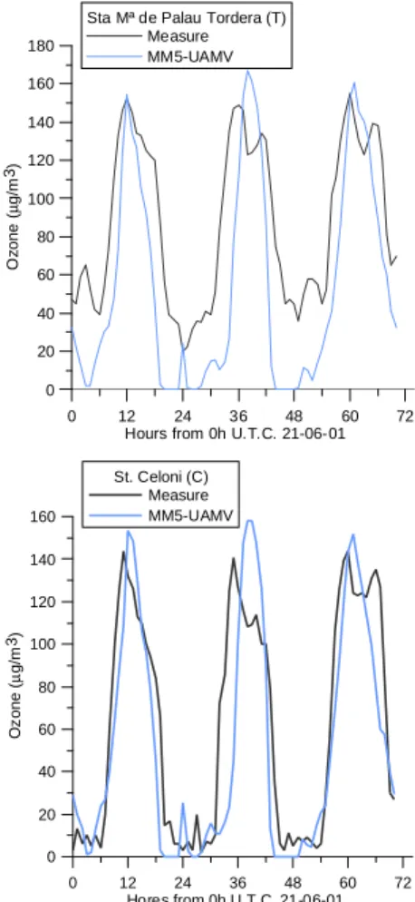
Figures 4, 5 and 6 compare the 3-day series of modelled ozone concentrations by UAMV with those observed at the six monitoring stations inside the domain. Concen-trations on the lowest level of the model, which is approximately 25 m, are compared

20

with the ambient data. Figures 4, 5 and 6 show the graphical validation of the MM5-UAMV performance for 72 h, except for the Manlleu station (M), where, due to several problems, data were only available for the first 40 h (Fig. 6). Qualitatively, the model simulates the ozone patterns reasonably well, particularly at the Granollers (G) station (Fig. 4). The low night values at the St. Celoni (C) (Fig. 5) and Granollers (G) stations

25

were simulated well, as was the strong increment between the night time minimum and the day time peak. However, at Sta. Ma de Palautordera (T) (Fig. 5), the model overpredicted the night time minimum ozone concentration, perhaps because of the rural nature of the station and the lack of precursors at night time. In the day time, the

(16)

ACPD

4, 1855–1885, 2004

model simulated the peak ozone concentrations quite accurately, especially in Vic (V) and Manlleu (M) (Fig. 6). As there are often high ozone values at these stations, this was one of the main goals of the simulation. Most of the stations in this study are closer to the boundary than those at Vic (V) and Manlleu (M) and, although the peak ozone concentrations were not simulated so accurately, we considered the slight mismatch in

5

peak ozone concentrations to be quite normal in current models. A larger domain may reduce the influence of the contour on these cells.

As well as graphical methods, we used eight statistical criteria (Jiang et al., 1998) to evaluate the results in Table 1. The negative values of mean bias and relative mean bias indicate that the model tends to underestimate ozone concentration. This

under-10

estimation may be due to the low values estimated by the model at nightime, since the model estimates the peak ozone concentration well. We can see in Table 1 that the statistics related to the maximum concentration bias are small and positive. When the relative mean gross error was compared in other simulations e.g. in Jiang et al. (1998), a value of 34.8% was assigned to the CALGRID model and a value of 36.9% was

as-15

signed to the UAMV model in a four-day simulation. In our simulation, relative mean gross error was 36.6% for MM5-UAMV, which is the order of magnitude of the other two modelling systems. Our results were very good when we analysed the agreement of the peak ozone concentrations. An average station peak normalized error of 5.6% improved the results from these other simulations.

20

6. Models comparison

Because the box model predicted ozone only in La Plana, more specifically in the Vic area, we can compare the two models only in Vic (V). There are many differences between the models, but the greatest difference is the extension of the domains. While the box model was only used for forecasting in La Plana, the grid model was more

25

widely used and shows the ozone in areas where there were no measurements. Also, the box model has been widely used as a forecasting tool. As it has been tested more

(17)

ACPD

4, 1855–1885, 2004

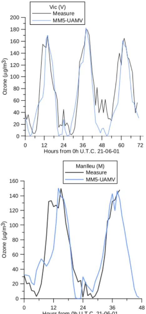
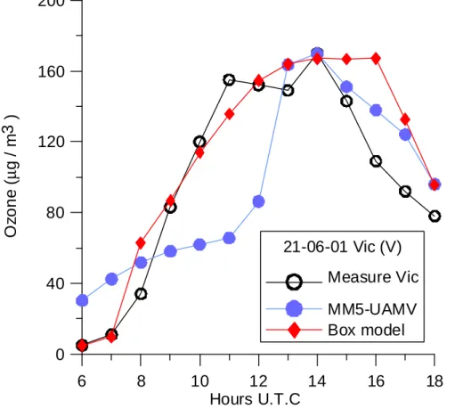
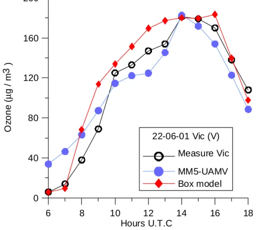
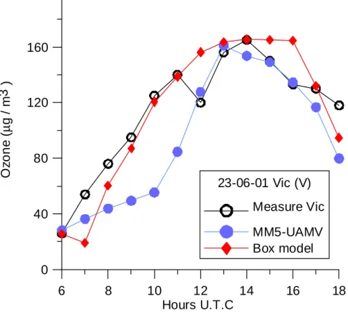
often it has been improved by slight modifications and is now a model that represents real ozone concentrations. The grid model, on the other hand, is in its first stage of development and needs more work and more simulations to become an effective tool that provides accurate and reliable forecasts of ozone concentration. However, we have made a preliminary comparison. Figures 7, 8 and 9 show the daily ozone

5

values predicted by both models and ozone measurements in Vic (V). Both models reproduced the ozone peak for the three days. However, the box model adjusted the measurements better during most of the daytime hours, while the grid model had a similar agreement only for 22 June. These discrepancies may be due to the fact that the box model has been specifically adjusted for the Vic area, while the grid model

10

represents the spatial distribution of ozone concentration in a larger domain, so it is more difficult to obtain an accurate diurnal concentration pattern. In addition to the graphical comparison, we have calculated some statistics for each model but, as the periods evaluated are different, the results may not be representative enough. In any case, we found that for the box model over the summer 2001 maximum concentration

15

accuracy was 16 µg/m3and bias was 3 µg/m3, and that for the grid model for the three days and the six stations considered in this study, maximum concentration accuracy was 7 µg/m3and bias was 2 µg/m3.

7. Conclusions

The aim of this paper was to apply two models over an area characterized by a complex

20

orography and affected by the presence of a nearby industrial area in which a sea breeze advects ozone and precursors to produce high ozone levels.

We analyzed the performances of a box model and a grid model in this area during different periods.

The box model was applied during the summer of 2001 in a nonoperative way but it

25

was used in the summer of 2003 as a forecasting tool. This helped to adjust the model specifically for this area and the results over this longer period are quite satisfactory.

(18)

ACPD

4, 1855–1885, 2004

Daily application of this model has shown that the main sources of error are indeter-mination in the emission model and in the height of the box model, but mainly in the cloudiness fraction, which is not accurately forecasted by the meteorological model.

The grid model was used during an ozone episode on three days of the summer of 2001. Although this model is only in its first stage of development, our results

demon-5

strate its capability as its performance was good over the area we studied. Grid models take into account a wider area and can therefore forecast ozone concentrations in sev-eral locations. This requires control and quantification in order to assess the scale of ozone impacts and develop control strategies. Although the performance of the model was tested for only a short period, we found that it was highly sensitive to boundary

10

conditions and only slightly sensitive to initial conditions. We therefore made a great ef-fort to adjust the model’s boundary conditions, especially those regarding hydrocarbon speciation. We believe the performance of the model would improve if a larger domain were used. This would reduce the boundary effects because the La Plana area would not be so close. Another way to improve performance is to execute a nested simulation.

15

This would require a great effort because a vast domain would have to be modelled. However, the model would be more operative because the boundary conditions for the inner domain (which would include La Plana) would come from this vast domain.

The comparison of the two models for the episode days showed good agreement between them and the measurement station. Although the box model reproduce the

20

daily ozone behaviour better than the grid model, both maximum values are really close to the peak ozone measured.

To conclude, we should stress that we validated and compared the whole modelling systems, not just the photochemical models. The modelling system includes the mete-orological model, the emission system and the photochemical model. In this way, we

25

have demonstrated two systems with sufficient accuracy for predicting ozone concen-trations.

Acknowledgements. The forecasting project was supported by the “Departament de Medi

(19)

ACPD

4, 1855–1885, 2004

REN2003-03436/CLI. The authors are grateful to the very competent help of the “Medi Ambient” (Environment) Department technicians, especially Carme Call ´es, Sonia S ´anchez and Joaquim Cot.

Edited by: J. Brandt

5

References

Alarc ´on, M., Alonso S., and Cruzado A.: Atmospheric trajectory models for simulation of long-range transport and diffusion over the Western Mediterranean, J. Env. Sc. & Health, A30, 9, 1973–1994, 1995.

Alarc ´on, M. and Alonso, S.: Computing 3-D atmospheric trajectories for complex orography:

10

application to a case study of strong convection in the western Mediterranea, Computers & Geosciences, 27, 583–596, 2001.

Blackadar, A. K.: Modelling the nocturnal boundary layer. Third Symposium on Atmospheric Turbulence, Diffusion and Air Quality, Raleigh, NC, 19–22 October, American Meteorological Society, 46–49, 1976.

15

Blackadar, A. K.: Modelling pollutant transfer during daytime convection, Fourth Symposium on Atmospheric Turbulence, Diffusion and Air Quality, Reno, NV, 15–18 January, American Meteorological Society, 443–447, 1979.

Berman, S., Ku, J. Y., Zhang, J., and Trivikrama, R.: Uncertainties in estimating the mixing depth – Comparing three mixing depth models with profiler measurements, Atmos. Env., 31,

20

18, 3023–3039, 1997.

Biswas, J., Hogrefe, C., Rao, S.T., Hao, W., and Sistla, G.: Evaluating the performance of regional-scale photochemical modeling systems, Part III-Precursor predictions, Atmos. Env., 35, 6129–6149, 2001.

Biswas, J., and Rao, S. T.: Uncertainties in episodic ozone modelling stemming from

uncertain-25

ties in the meteorological fields, J. Appl. Meteor., 40, 117–136, 2001.

EPA: Guideline for developing an ozone forecasting program. Office of Air Quality Planning and Standards, Research Triangle Park, N.C., EPA-254/R-99-009, July, 1999.

Chalita, S., Hauglustaine, D., LeTreut, H., and Muller, J.-F.: Radiative forcing due to increased tropospheric ozone concentrations, Atmos. Env., 30, 1641–1646, 1996.

(20)

ACPD

4, 1855–1885, 2004

Codina, B., Aran, M., Young, S., and Reda ˜no, A.: Prediction of a Mesoscale Convective Sys-tem over Catalonia (Northeastern Spain) with a Nested Numerical Model, Meteorology and Atmospheric Physics, 62, 9–22, 1997.

EMEP/CORINAIR: Emission Inventory Guidebook – 3rd edition, 1999.

Department of Territorial Policy and Public Works of Spain: Monthly Traffic Statistics:

Es-5

tad´ıstica mensual de tr`afic, 2000.

Directorate General for Traffic: Anuario estad´ıstico general, 2001.

Dudhia, J., Gill, D., Guo, Y. -R., Manning, K., Wang, W., and Chiszar, J.: PSU/NCAR Mesoscale Modeling System Tutorial Class Notes and User’s Guide: MM5 Modeling System Version

3, National Center for Atmospheric Research, http://www.mmm.ucar.edu/mm5/documents/

10

MM5 tut Web notes/TutTOC.html, 138, 2000.

Finlayson-Pitts, B. J. and Pitts, J. N.: Chemistry of the upper and lower atmosphere, Academic Press, 2000.

Gery, M., Whitten, G. Z., Killus, J. P., and Dodge, M. C.: A photochemical kinematics mecha-nism for urban and regional scale computer modeling, Journal Geophysical Research, 94,

15

12, 925–946, 1989.

Gery, M. W. and Crouse, R. R.: User’s Guide for Executing OZIPR, U.S. Environmental Protec-tion Agency, Research Triangle Park, N.C., EPA-9D2196NASA, 1990.

Grell, G. A.: Prognostic Evaluation of Assumptions used by Cumulus Parameterization, Monthly Weather Review, 121, 764–787, 1993.

20

Grossi, P., Thunis, P., Martilli, A., and Clappier, A.: Effect of sea breeze on air pollution in the greather Athens area. Part II: Analysis of different Emissions Scenarios, J. Appl. Meteor., 39, 4, 563–575, 2000.

Guderian, R., Tingey, D. T., and Rabe, R.: Effects of photochemical oxidants on plants in Air Pollution by Photochemical Oxidants, edited by Guderian, R., 129–333, Springer, Berlin,

25

1985.

Hewit, C., Lucas, P., Wellburn, A., and Fall, R.: Chemistry of ozone damage to plants, Chemistry and Industry, 15, 478–481, 1990.

Hogrefe, C., Rao, S. T., Kasibhatla, P., Kallos, G., Tremback, C. J., Hao, W., Olerud, D., Xiu, A., McHenry, J., and Alapaty, K.: Evaluating the performance of regional-scale photochemical

30

modelling systems: Part I- metorological predictions, Atmos. Env., 35, 4159–4174, 2001.

Jiang, W., Hedley, M., and Singleton, D. L.: comparison of the MC2/CALGRID and

(21)

ACPD

4, 1855–1885, 2004

Atmos. Env., 32, 17, 2969–2980, 1998.

Kaplan, M. L., Zack, J. W., Wong, V. C., and Tuccillo, J. J.: Initial results from a mesoscale atmospheric simulation system and comparisons with an AVE-SESAME I data set, Monthly Weather Review, 110, 1564–1590, 1982.

Ligocki, M. P. and Whitten, G. Z.: Modelling of Air Toxics with the Urban Airshed model, Air and

5

Waste Management Association 85th Annual Meeting and Exhibition, Kansas City, Missouri, paper 92-84.12, 1992.

Ligocki, M. P., Schulhof, R. R., Jackson, R. E., Jimenez, M. M., Whitten, G. Z., Wilson, G. M., Myers, T. C., and Fieber, J. L.: Modelling the Effects of Reformulated Gasoline on Ozone and Toxics Concentration in Baltimore and Houston Areas, SYSAPP-92/127, 1992.

10

Lippmann, M.: Health effects of tropospheric ozone, Environ. Sci. Technol., 25, 12, 1991. McCree, K. J.: Test of current definitions of photosynthetically active radiation against leaf

pho-tosynthetically active radiation against lead photosynthesis data, Agricultural Meteorology, 10, 442–453, 1972.

Ministry of Public Works of the Spanish Government: Monthly traffic statistics, Estad´ıstica

men-15

sual de tr ´afico, 2000.

Pierce, T., Geron, C., Bender, L., Dennis, R., Tonnesen, G. and Guenter, A.: Influence of iso-prene emissions on regional ozone modeling, J. Geophys. Res., 103, D 19, 25 611–25 629, 1998.

Sagebiel, J. C., Zielinska, B., Pierson, W. R., and Gertler, A. W.: Real-world emissions and

20

calculated reactivities of organic species from motor vehicles, Atmos. Env., 30, 12, 2287– 2296, 1996.

Silibello, C., Calori, G., Brusasca, G., Catenacci, G., and Finzi, G.: Application of a photochem-ical grid model to Milan metropolitan area, Atmos. Env., 32, 11, 2025–2038, 1998.

Soler, M. R., Hinojosa, J., Bravo, M., Pino, D., and Vil `a Guerau de Arellano, J.: Analizing the

25

basic features of different complex terrain flows by means a Doppler Sodar and a numerical model: Some implications to air pollution problems, Meteorology and Atmospheric Physics, Meteorology and Atmospheric Physics, 85, 1–3, 141–154, 2003.

Statistical Institute of Catalonia: Anuari Estad´ıstic, 2000.

Stockwell, R. W., Middleton, P., and Chang J. S.: The second generation Regional Acid

depo-30

sition model. Chemical mechanism for regional air quality modeling, J. Geophys. Res., 95, 16343–16367, 1990.

(22)

ACPD

4, 1855–1885, 2004

Distances. J. Atmos. Sc., 41, 3351–3367, 1984.

Stull, R. B. and Hasegawa, T.: Transilient Turbulence Theory, Part II: Turbulence Adjustment, J. Atmos. Sc., 41, 3368–3379, 1984.

Stull, R. B. and Driedonks, A. G. M.: Applications of the Transilient Turbulence Parameterization to Atmospheric Boundary Layer Simulations, Boundary-Layer Meteorology, 40, 209–239,

5

1987.

Zack, J. W. and Kaplan, M. L.: Numerical simulations of the subsynoptic features associated with the AVE-SESAME I Case, Part I: The preconvective environment, Monthly Weather Review, 115, 2367–239, 1987.

(23)

ACPD

4, 1855–1885, 2004

Table 1. Statistics results for MM5-UAMV performance.

MM5-UAMV

Mean Bias (µg/m3) −13.2

Relative Mean Bias (%) −20.7

Mean Gross Error (µg/m3) 23.8

Relative Mean Gross Error (%) 36.6

Bias for maximums (µg/m3) 1.78

Average Station Peak Normalized Bias (%) 2.0

Accuracy for maximum (µg/m3) 7.23

(24)

ACPD

4, 1855–1885, 2004

Fig. 1. Orography of the studied area. The black points are the location of the measurement stations.

(25)

ACPD

4, 1855–1885, 2004

(26)

ACPD

4, 1855–1885, 2004

Print Version Interactive Discussion © EGU 2004 430 435 440 445 450 455 4605 4610 4615 4620 4625 4630 4635 4640 4645 4650 4655 20 40 60 80 100 120 140 160 180 MM5-UAMV simulation 22-6-2001 Ozone h 10 X UTM (km) Y U T M ( km) 430 435 440 445 450 455 4605 4610 4615 4620 4625 4630 4635 4640 4645 4650 4655 20 40 60 80 100 120 140 160 180 MM5-UAMV simulation 22-6-2001 Ozone h 15 X UTM (km) Y U T M ( km)

Fig. 3. Spatial distribution of ozone from UAMV simulation on 22 June left panel at 10:00 UTC and right panel at 15:00 UTC. The colour ozone scale is in µgm−3and the white rhombus show Vic location.

(27)

ACPD

4, 1855–1885, 2004

0 12 24 36 48 60 72

Hours from 0h U.T.C. 21-06-01 0 20 40 60 80 100 120 140 O z o n e ( µ g /m 3) Sabadell (S) Measure MM5-UAMV 0 12 24 36 48 60 72

Hours from 0h U.T.C. 21-06-01 0 20 40 60 80 100 120 140 O z o n e ( µ g /m 3) Granollers (G) Measure MM5-UAMV

Fig. 4. Hourly ozone measurement (black) and UAMV prediction (blue) for 21, 22 and 23 June 2001. The upper panel corresponds to Sabadell, and the lower to Granollers.

(28)

ACPD

4, 1855–1885, 2004

Hours from 0h U.T.C. 21-06-01 0 20 40 60 80 100 120 140 160 180 O z o n e ( µ g /m 3)

Sta Mª de Palau Tordera (T) Measure MM5-UAMV

0 12 24 36 48 60 72 Hores from 0h U.T.C. 21-06-01 0 20 40 60 80 100 120 140 160 O z o n e ( µ g /m 3) St. Celoni (C) Measure MM5-UAMV

Fig. 5. Hourly ozone measurement (black) and UAMV prediction (blue) for 21, 22 and 23 June 2001. The upper panel corresponds to Sta. Made Palau Tordera, and the lower to St. Celoni.

(29)

ACPD

4, 1855–1885, 2004

Hours from 0h U.T.C. 21-06-01 0 20 40 60 80 100 120 140 160 180 200 O z o n e ( µ g /m 3) Vic (V) Measure MM5-UAMV 0 12 24 36 48

Hours from 0h U.T.C. 21-06-01 0 20 40 60 80 100 120 140 160 O z o n e ( µ g /m 3) Manlleu (M) Measure MM5-UAMV

Fig. 6. Hourly ozone measurement (black) and UAMV prediction (blue). The upper panel corresponds to Vic, for 21, 22 and 23 June 2001, and the lower to Manlleu, for 21 and 22 June 2001.

(30)

ACPD

4, 1855–1885, 2004

6

8

10

12

14

16

18 Hours U.T.C

0

40

80

120

160

200 O

z

o

n

e

(

µ

g

/

m

3 )

21-06-01 Vic (V)

Measure Vic

MM5-UAMV

Box model

Fig. 7. Graphical comparison of ozone from measurement station (black), UAMV simulation (blue) and box model forecast (red), in Vic on 21 June 2001.