Dynamic reduced order modeling of entrained flow gasifiers

(1)

Dynamic Reduced Order Modeling of Entrained Flow Gasifiers

by

Rory F. D. Monaghan

B.E. (Honors), Mechanical Engineering (2002) National University of Ireland, Galway

MAY 0

5 2010

LIBRAR IES

S.M., Mechanical Engineering (2005)

Massachusetts Institute of Technology

Submitted to the Department of Mechanical Engineering in Partial Fulfillment of the Requirements for the Degree of

Doctor of Philosophy in Mechanical Engineering at the

MASSACHUSETTS INSTITUTE OF TECHNOLOGY

FEBRUARY 2010

0 2010 Massachusetts

/r,)

A

Signature of Autho ...

Department of Mechanical Engineering December 16, 2009

Certified by... ...

..r..-Ahmed F. Ghoniem Ronald C. Crane (1972) Professor Thesis Supervisor

A ccepted by ... ...

David E. Hardt Chairman, Department Committee on Graduate Students

(2)

(3)

Dynamic Reduced Order Modeling of Entrained Flow Gasifiers

by

Rory F. D. Monaghan

Submitted to the Department of Mechanical Engineering on December 16, 2009 in Partial Fulfillment of the Requirements for the Degree of Doctor of Philosophy in

Mechanical Engineering

ABSTRACT

Gasification-based energy systems coupled with carbon dioxide capture and storage technologies have the potential to reduce greenhouse gas emissions from continued use of abundant and secure fossil fuels. Dynamic reduced order models (ROMs) that predict the operation of entrained flow gasifiers (EFGs) within IGCC (integrated gasification combined cycle) or polygeneration plants are essential for understanding the fundamental processes of importance. Such knowledge can be used to improve gasifier reliability, availability and maintainability, leading to greater commercialization of gasification technology.

A dynamic ROM, implemented in Aspen Custom Modeler, has been developed for a range of EFGs. The ROM incorporates multiple feedstocks, mixing and recirculation, particle properties, drying and devolatilization, chemical kinetics, fluid dynamics, heat transfer, pollutant formation, slag behavior and syngas cooling. The ROM employs a reactor network model (RNM) that approximates complex fluid mixing and recirculation using a series of idealized chemical reactors. The ROM was successfully validated for steady-state simulation of four experimental gasifiers. The throughputs of these gasifiers range from 0.1 to 1000 metric tonnes per day (3 kWth - 240 MWth). Sensitivity analysis was performed to identify the parameters most important to ROM accuracy. The most important parameters are found to be those that determine RNM geometry, particle physical and kinetic properties, and slagging.

The ROM was used to simulate the steady-state and dynamic performance of a full-scale EFG system. In steady-state mode, the ROM was used to establish base case and fluxant requirements. The base case performance agreed with design specifications. Steady-state simulation was also used to determine important states for dynamic simulation. Six cases were examined in dynamic mode, including gasifier cold start. Dynamic results showed agreement with industrial experience for gasifier start-up times.

Thesis Supervisor: Ahmed F. Ghoniem Title: Ronald C. Crane (1972) Professor

(4)

(5)

ACKNOWLEDGEMENTS

I wish to sincerely thank my Thesis Supervisor, Professor Ahmed Ghoniem, and my Thesis Committee, Professor Janos Beer, Professor John Brisson, Mr. Randy Field and Professor Greg McRae. I must single out Professors Ghoniem and Brisson, who have supported me through teaching and research for almost my entire time at MIT. Their dedication and conscientiousness made it possible for me to pursue what I have come to regard as my dream-project to the best of my abilities. Randy Field, more than anyone else, was directly involved in the day-to-day development of the model, especially in the early day-to-days of helping me find my feet with ACM. I have no doubt that my experience has been richer for the help and guidance I received from Randy, and from James Goom at AspenTech. Professors Beer and McRae have immense experience in the fields of combustion, gasification, simulation and experimentation, and were always available for advice and assistance.

The sponsors of this work, BP, have been all a graduate student could hope for in an industrial sponsor. This work has benefitted hugely from the contributions of George Huff, David Jeffers, Liguang Wang and Mike Desmond. They gave me the freedom to pursue my own avenues of investigation, while providing invaluable insight into the practical, real-world applications and requirements of the work. I also could not have wished for better, more capable work-mates than my colleagues in gasification modeling, Mayank Kumar, Simcha Singer and Dr. Cheng Zhang. The same can be said of my lab-mates in the Reacting Gas Dynamics Lab. The rapid expansion of the group is a testament to the high quality of work produced by this team. It has been a pleasure and a privilege to work with Professor Ghoniem, Lorraine Rabb and the rest of the RGD group.

But academia is only one aspect of my time at MIT. Of at least equal importance are the friendships I built during my 6 years here. My friends have always been there for me, to lift me up and occasionally bring me back down to earth! I have made far too many good friends to list them all so I will simply thank the Unbelievables, the lads of 32 Adrian, Chez Jay and 7D Tang, the Irish Association, MechE coffee hour, basketball and grad office, the Cryo Lab, the boys at the Field, 2.005/2.006, my fellow GSC ski-trippers, the Energy Club, and the ISO. You all made my time here the most memorable and rich of my life. But I would not have come to MIT in the first place were it not for my family, Anne, Paul and Fergal. I owe them a huge debt of gratitude for everything they have done for me in my life and during my time here. Finally I wish to thank my amazing fiancee, Sinead. For more than four years, Sinead has endured my PhD with super-human patience, loyalty and commitment. I cannot believe how much you have done for me throughout my time here, and I hope you realize just how much you helped me get through. I dedicate this work to Sinead, Anne, Paul and Fergal.

(6)

(7)

LIST OF FIGURES

Figure 1-1: W orld energy dem and to 2030 ... 26

Figure 1-2: W orld CO2 emissions to 2030... 26

Figure 1-3: Geological storage options for CO2 (from [3]) ... 29

Figure 1-4: Levelized costs of electricity for fossil plants with and without CCS...31

Figure 1-5: 2007 solid-feedstock-derived syngas capacity by product ... 33

Figure 1-6: The gasifier in a highly simplified plant schematic...34

Figure 1-7: (a) GE (radiant), (b) CoP E-GAS and (c) SCGP gasifiers ... 40

Figure 1-8: Times between gasifier switches and shutdowns for 1984-2004 ... 47

Figure 2-1: Particle trajectories, stream lines and zero axial velocity boundaries for an axially-fired coal combustor (reproduced from [1])...56

Figure 2-2: Flow field and RNM for a one-stage gasifier...57

Figure 2-3: Flexible RNM for a one- or two-stage gasifier with syngas cooling ... 60

Figure 2-4: Model implementation using submodels ... 70

Figure 2-5: Mass balance for devolatilization submodel...75

Figure 2-6: Heat transfer term s evaluated... 88

Figure 2-7: Nitrogen global reaction mechanism ... 90

Figure 2-8: Trends of gas phase sulfur chemistry using the Savel'ev submodel...92

Figure 2-9: Sulfur global reaction mechanism ... 93

Figure 2-10: Mass and energy flows for one- and two-layer slag submodels ... 94

Figure 2-11: Syngas cooling subm odel... 97

Figure 2-12: Node-spacings for PFRs used in the ROM...100

Figure 3-1: Example of sensitivity analysis results...115

Figure 3-2: 2 tpd MHI gasifier schematic and characteristics ... 116

Figure 3-3: Reactor Network Model for 2 tpd MHI gasifier ... 120

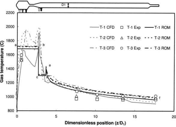
Figure 3-4: Temperature profiles for Coal M from CFD, experiments and ROM. 122 Figure 3-5: Temperature profiles for Coal T from CFD, experiments and ROM .123 Figure 3-6: Syngas composition from CFD, experiments and ROM ... 124

Figure 3-7: Carbon conversion from CFD, experiments and ROM...125

Figure 3-8: Char mass flow rate from CFD, experiments and ROM ... 126

Figure 3-9: Syngas heating value from CFD, experiments and ROM...127

Figure 3-10: Cold gas efficiency from CFD, experiments and ROM...127

Figure 3-11: Ultimate analysis profile for Test M-1 for MHI lab-scale gasifier ... 129

Figure 3-12: Proximate analysis profiles for MHI lab-scale gasifier...129

(13)

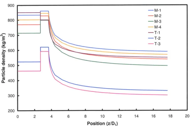
Figure 3-14: Particle bulk density profiles for MHI lab-scale gasifier...131

Figure 3-15: Particle mass profiles for MHI lab-scale gasifier ... 131

Figure 3-16: Particle volume fraction profiles for MHI lab-scale gasifier ... 132

Figure 3-17: Extrinsic heterogeneous reaction rate profiles for MHI lab-scale gasifier ... 1 3 3 Figure 3-18: Wall heat flux profiles for MHI lab-scale gasifier...134

Figure 3-19: Sensitivity of MHI exit carbon conversion to input parameters ... 135

Figure 3-20: Sensitivity of MHI temperature profile to selected parameters...137

Figure 3-21: 0.1 tpd CSIRO gasifier schematic and characteristics...140

Figure 3-22: Reactor Network Model for 0.1 tpd CSIRO gasifier ... 143

Figure 3-23: Gas composition profile comparisons for CRC299 ... 145

Figure 3-24: Carbon conversion profile comparisons for CRC299...145

Figure 3-26: Carbon conversion profile comparisons for CRC358 ... 146

Figure 3-31: Ultimate analysis profile for test CRC252 for CSIRO lab-scale gasifier ... 1 4 9 Figure 3-32: Proximate analysis profiles for CSIRO lab-scale gasifier ... 150

Figure 3-33: Particle bulk density profiles for CSIRO lab-scale gasifier ... 151

Figure 3-34: Particle mass profiles for CSIRO lab-scale gasifier ... 151

Figure 3-35: Particle volume fraction profiles for CSIRO lab-scale gasifier ... 152

Figure 3-36: Particle internal surface area profiles for CSIRO lab-scale gasifier... 154

Figure 3-37: Heterogeneous intrinsic reaction rate profiles for CSIRO lab-scale g a sifier ... 1 5 4 Figure 3-38: Heterogeneous extrinsic reaction rate profiles for CSIRO lab-scale g a sifie r ... 1 5 5 Figure 3-39: Effectiveness factor profiles for heterogeneous reactions for CSIRO lab-scale g a sifier ... 15 5 Figure 3-40: Resistivities of film diffusion and pore diffusion-reaction for test C R C 3 5 8 ... 15 7 Figure 3-41: Resistivities of film diffusion and pore diffusion-reaction for test C R C 2 5 2 ... 1 5 8 Figure 3-42: Temperature profiles for CSIRO lab-scale gasifier...159

(14)

Figure 3-43: Wall heat flux profiles for CSIRO lab-scale gasifier...160

Figure 3-44: Sensitivity of CSIRO exit carbon conversion to input parameters ... 162

Figure 3-45: 1 tpd BYU gasifier schematic and characteristics...166

Figure 3-46: Reactor Network Model for 1 tpd BYU gasifier...169

Figure 3-47: Gas composition profile comparisons for 1 tpd BYU gasifier...171

Figure 3-48 Nitrogenous pollutant profile comparisons for 1 tpd BYU gasifier.. 172

Figure 3-49 : Sulfurous pollutant profile comparisons for 1 tpd BYU gasifier ... 173

Figure 3-50: Particle ultimate analysis profile for BYU lab-scale gasifier ... 174

Figure 3-51: Particle proximate analysis profile for BYU lab-scale gasifier ... 175

Figure 3-52: Particle bulk density profile for BYU lab-scale gasifier ... 176

Figure 3-53: Particle mass profile for BYU lab-scale gasifier ... 176

Figure 3-54: Particle volume fraction profile for BYU lab-scale gasifier ... 177

Figure 3-55: Heterogeneous extrinsic reaction rate profiles for BYU lab-scale g a sifie r ... 1 7 8 Figure 3-56: Temperature profiles for BYU lab-scale gasifier ... 179

Figure 3-57: Wall heat flux profiles for BYU lab-scale gasifier ... 180

Figure 3-58: Sensitivity of BYU exit carbon conversion to input parameters...182

Figure 3-59: Sensitivity of BYU exit NH3:HCN ratio to nitrogenous pollutant p ara m eters ... 18 4 Figure 3-60: Sensitivity of BYU exit H2S:SO2 ratio to sulfurous pollutant p a ram eters ... 18 5 Figure 3-61: 1000 tpd GE gasifier schematic and characteristics...189

Figure 3-62: GE gasifier schematic from Saint-Gobain website [12]...190

Figure 3-63: Reactor Network Model for 1000 tpd GE gasifier ... 192

Figure 3-64: Temperature profiles for 1000 tpd GE gasifier design case ... 194

Figure 3-65: Exit carbon conversions for 1000 tpd GE gasifier ... 195

Figure 3-66: Syngas compositions for ROM with and without reaction in the RSC ... 1 9 6 Figure 3-67: Ultimate analysis profile for Test 1 for GE pilot-scale gasifier ... 197

Figure 3-68: Proximate analysis profiles for GE pilot-scale gasifier ... 198

Figure 3-69: Gas composition profiles for Test 1 for GE pilot-scale gasifier ... 199

Figure 3-70: Particle bulk density profiles for GE pilot-scale gasifier ... 200

Figure 3-71: Particle mass profiles for GE pilot-scale gasifier ... 200

Figure 3-72: Particle volume fraction profiles for GE pilot-scale gasifier ... 201 Figure 3-73: Heterogeneous extrinsic reaction rate profiles for GE pilot-scale gasifier ... 2 0 2

(15)

Figure 3-74: Wall heat flux profiles for GE pilot-scale gasifier ... 203

Figure 3-75: Sensitivity of GE exit carbon conversion to input parameters ... 204

Figure 3-76: Sensitivity of GE exit temperature to input parameters...205

Figure 3-77: Sensitivity of RSC exit temperature to RSC parameters...208

Figure 3-78: Sensitivity of RSC exit H2:CO ratio to RSC parameters ... 208

Figure 4-1: Schematic of gasifier and syngas cooler for Reference Plant...219

Figure 4-2: Reactor Network Model for GE gasifier in Reference Plant ... 221

Figure 4-3: Temperature profiles for GE gasifier in Reference Plant ... 223

Figure 4-4: Temperature profiles for RSC in Reference Plant ... 224

Figure 4-5: Gas composition profiles for GE gasifier in Reference Plant ... 225

Figure 4-6: Gas composition profiles for RSC in Reference Plant...225

Figure 4-7: Nitrogen species profiles for GE gasifier in Reference Plant ... 226

Figure 4-8: Sulfur species profiles for GE gasifier in Reference Plant ... 227

Figure 4-9: Composition of Illinois No. 6 coal-ash...228

Figure 4-10: Temperature-viscosity curves for Illinois No. 6 slag with fluxant a d d itio n ... 2 3 0 Figure 4-11: Slag viscosity, velocity, thickness and mass flow rate profiles for GE gasifier in R eference P lant...231

Figure 4-12: Recording positions for important dynamic ROM simulation outputs ... 2 4 1 Figure 4-13: Temperature history for Case 1: Removal of Fluxant...243

Figure 4-14: Quenched gas composition history for Case 1: Removal of Fluxant .243 Figure 4-15: Syngas production history for Case 1: Removal of Fluxant ... 244

Figure 4-16: Slag behavior history for Case 1: Removal of Fluxant...244

Figure 4-17: Temperature history for Case 2: Load Following...246

Figure 4-18: Quenched gas composition history for Case 2: Load Following ... 247

Figure 4-19: Syngas production history for Case 2: Load Following...247

Figure 4-20: Slag behavior history for Case 2: Load Following...248

Figure 4-21: Temperature history for Case 3: Feed Switching...249

Figure 4-22: Quenched gas composition history for Case 3: Feed Switching ... 250

Figure 4-23: Slag behavior history for Case 3: Feed Switching ... 250

Figure 4-24: Pollutant species history for Case 3: Feed Switching...251

Figure 4-25: Temperature history for Case 4: Coal-Petcoke Co-firing ... 253

Figure 4-26: Quenched gas composition history for Case 4: Coal-Petcoke Co-firing ... 2 5 3 Figure 4-27: Syngas production history for Case 4: Coal-Petcoke Co-firing ... 254

(16)

Figure 4-28: Slag behavior history for Case 4: Coal-Petcoke Co-firing ... 254

Figure 4-29: Pollutant species history for Case 4: Coal-Petcoke Co-firing...255

Figure 4-30: Temperature history for Case 5: Coal-Biomass Co-firing...257

Figure 4-31: Quenched gas composition history for Case 5: Coal-Biomass Co-firing ... 2 5 7 Figure 4-32: Syngas production history for Case 5: Coal-Biomass Co-firing...258

Figure 4-33: Slag behavior history for Case 5: Coal-Biomass Co-firing...258

Figure 4-34: Pollutant species history for Case 5: Coal-Biomass Co-firing ... 259

Figure 4-35: Temperature history for Case 6: Gasifier Cold Start ... 261

Figure 4-36: Refractory heating rate histories for Case 6: Gasifier Cold Start ... 262

Figure 4-37: Gasifier exit gas composition history for Case 6: Gasifier Cold Start263 Figure 4-38: Syngas production history for Case 6: Gasifier Cold Start ... 264

Figure 4-39: Slag behavior history for Case 6: Gasifier Cold Start ... 266

Figure 4-40: Pollutant species history for Case 6: Gasifier Cold Start...267

Figure 5-1: Flexible RNM for a one- or two-stage gasifier with syngas cooling .... 273

Figure 5-2: ROM and CFD predictions and experimental measurement of temperature profiles for Coal M in MHI gasifier ... 277

Figure 5-3: ROM prediction and experimental measurement of gas composition profiles for test CRC252 in CSIRO gasifier...277

Figure 5-4: ROM prediction and experimental measurement of gas composition profiles for B Y U gasifier ... 278

Figure 5-5: ROM prediction of temperature profiles for BYU gasifier ... 278

Figure 5-6: ROM-predicted heterogeneous extrinsic reaction rate profiles for MHI g a sifie r ... 2 8 1 Figure 5-7: ROM-predicted heterogeneous extrinsic reaction rate profiles for BYU g a sifie r ... 2 8 1 Figure 5-8: ROM-predicted heterogeneous extrinsic reaction rate profiles for GE g a sifier ... 2 8 2 Figure 5-9: ROM-predicted particle internal surface area profiles for CSIRO gasifier ... 2 8 3 Figure 5-10: ROM-predicted heterogeneous intrinsic reaction rate profiles for C S IR O gasifier ... 284

Figure 5-11: ROM-predicted resistivities of film diffusion and pore diffusion-reaction for C SIR O test CR C 358 ... 284

Figure 5-12: ROM-predicted resistivities of film diffusion and pore diffusion-reaction for C SIR O test C R C 252 ... 285

(17)

Figure 5-13: ROM-predicted effect of fluxant on slag temperature-viscosity profile for full-scale G E gasifier ... 289

(18)

LIST OF TABLES

Table 1-1: Currently and planned CCS projects ... 30

Table 1-2: Characteristics of gasifier fam ilies ... 35

Table 1-3: Commercial entrained flow gasifier characteristics ... 41

Table 1-4: Gasifier shutdowns for January-September 2004 ... 47

Table 1-5: The roles of simulation in addressing current EFG problems...48

Table 1-6: Important characteristics of gasifier models that incorporate RNMs...51

Table 2-1: Switches used in flexible one- or two-stage RNM ... 62

Table 2-2: Conservation equations for 1-D PFR (part 1) ... 67

Table 2-3: Calculated solid phase properties... 73

Table 2-4: Source terms for solid phase proximate and ultimate species ... 76

Table 2-5: Homogeneous reaction rate expressions...77

Table 2-6: Semi-global mechanisms for heterogeneous gasification reactions (part 1) ... 8 0 T able 2-7: V iscous interactions... 85

Table 2-8: Reactions, expression and parameters for nitrogen submodel...90

Table 3-1: Experimental data for entrained flow gasifiers...110

Table 3-2: Input parameters and base case values for the ROM ... 114

Table 3-3: Test conditions for 2 tpd M HI gasifier ... 118

Table 3-4: Specifications of coal tested in 2 tpd MHI gasifier...118

Table 3-5: Kinetic rate parameters for Coal NL...119

Table 3-6: Calculations for recycled char proximate and ultimate analyses ... 121

Table 3-7: Sensitivity of MHI exit carbon conversion to input parameters ... 136

Table 3-8: Test conditions and coal specification for 0.1 tpd CSIRO gasifier...141

Table 3-9: Kinetic rate parameters for CSIRO gasifier test coals from [3]...142

Table 3-10: Sensitivity of CSIRO exit carbon conversion to input parameters .... 163

Table 3-11: Test conditions and coal composition for 1 tpd BYU gasifier...167

Table 3-12: Original and tuned pollutant reaction frequency factors...173

Table 3-13: Sensitivity of BYU exit carbon conversion to input parameters...183

Table 3-14: Sensitivity of BYU exit NH3:HCN and H2S:SO2 ratios to pollutant p a ram eters ... 18 5 T able 3-15: G E gasifier sizes... 188

Table 3-16: Test conditions and results for Cool Water gasifier ... 191 Table 3-17: Sensitivity of GE carbon conversion and exit temperature to input p ara m eters ... 2 0 6

(19)

Table 3-18: Sensitivity of RSC exit temperatures and H2:CO ratio to RSC p aram eters ... 2 0 9 Table 4-1: Flow rates and conditions for Reference Plant gasifier and syngas cooler

... 2 1 9 T able 4-2: Feedstock description ... 220 Table 4-3: Gasifier operations for dynamic ROM simulation...232 Table 4-4: Important properties of feedstocks used in dynamic ROM simulation 234 Table 4-5: Test matrix for dynamic ROM simulations ... 238 Table 5-1: Total heat capacities of gasifier and syngas cooler components...291

(20)

NOMENCLATURE

Capital Letters

A Area (m2

) or Frequency factor (kg/m2_/atm"/s)

A' Area per unit volume (m2_/m3₎

ACH Stoichiometric ratio of air to char (kg/kg) AcO Stoichiometric ratio of air to coal (kg/kg) B Length scale for radiation heat transfer (m)

c Particle conversion

CD Drag coefficient

D _{Diffusivity (m}2_/s)

E Activation energy (kJ/kmol)

F~ Viscous frictional force per unit volume (N/m3) K _{Equilibrium constant or Absorption coefficient (m)}

L Length (m)

M Reaction rate multiplier

N Number density (m~)

Nu Nusselt number

P Pressure (atm, bar, MPa or Pa) Peh Peclet number for heat transfer Pe. Peclet number for mass transfer

Heat transfer rate per unit axial length (kW/m) Heat transfer rate per unit area (kW/m2₎

R Rate of chemical reaction (kg/m3/s)

h Rate of chemical reaction (kmol/m3/s) 91 Ideal gas constant (kJ/kmol/K)

Ra Rayleigh number

Re Reynolds number

S Rate of species formation (kg/m3_{) or Swirl number}

s1

Sensitivity of output (o) to input (z)

Sh Sherwood number T Temperature (K) v Volume (m3 ) x Mass fraction (kg/kg) Mole fraction Yield (kg/kg) CO-CO2 ratio (kmol/kmol) at particle surface

Lowercase Letters

a Specific area (m2_/kg) act Actual

c, Specific heat capacity (kJ/kg/K)

d Diameter (m)

f Friction factor

Correction factor

Mass fraction of flow leaving ERZ to enter JEZ directly

fc y z

fc.

(21)

fN fsiag g h ki k k(T) I m n n r r rp. S t U V w x

Greek Letters

Recirculation ratio (kg/kg) or switch

Particle density evolution parameter or Slag surface angle (deg) or Inverse film temperature (K-)

Chemical species Thickness (m)

Arbitrarily small number

Volume fraction (m3/m3_{) or Porosity (m}3_/m3_{) or emissivity} Mechanism factor or Thiele Modulus

Effectiveness factor

Mass transfer coefficient (kmol/m2_/s)

Air ratio (kg/kg)

Gasifier air ratio (kg/kg) Dynamic viscosity (Pa.s) Jet expansion angle (deg) Density (kg/m3)

Molar density (kmol/m3)

Stefan-Boltzmann constant (5.67x10~" kW/m2/K4) Stoichiometric coefficient or Kinematic viscosity (m2_/s)

Particle roughness (-) or Wall roughness (m) Particle structural parameter

Mass fraction of devolatilized nitrogen evolving as HCN Slag deposition factor

Gravitational acceleration (m/s2₎

Enthalpy (kJ/kg) or Heat transfer coefficient (kW/m2_/K)

Enthalpy (kJ/kmol) Conductivity (kW/m/K)

Reaction rate constant ((kg/m 2_{/atm"/s) for heterogeneous)}

Length per unit mass (m/kg) Mass (kg)

Mass flow rate (kg/s)

Mass flow rate per unit axial length (kg/m/s) Mass flow rate per unit area (mass flux) (kg/m2_/s)

Heterogeneous reaction order Molar flux (kmol/m2_/s)

Radius (m)

Resistivity (s/m)

Average pore radius (m) Silica ratio

Time (s) or Thickness (m) Internal energy (kJ/kg) Velocity (m/s)

Mole weight (kg/kmol) Axial position (m)

(22)

Subscripts

A Molecular diffusion act Actual amb Ambient c Characteristic C Carbon or Concentration CS Cross section cond Conduction conv Convection

CV _{Critical value (slag temperature)} dev Devolatilization d Diameter diff Diffusion dry Drying e Electric eff Effective ex Extrinsic

exit Gasifier exit

ext External

f Formation or Film

fus Fusion (heat of)

g Gas

H Hydrogen (elemental)

HT Heat transfer

i Gas phase species

in Intrinsic

int Internal

j

Solid phase species

(proximate)

k _{Solid phase species (ultimate)}

K Knudsen diffusion

1 Wall layer (i.e. firebrick (refractory), insulating brick, steel wall)

liq Liquid

m Heterogeneous reaction

M Moisture

n Homogeneous reaction

p Particle

pore Intraparticle pore

r Recirculated rad Radiation ref Refractory rxn Reaction s Particle surface sens Sensible

slag Slag on wall

slagging Slag transport to wall

sol Solid

th Thermal

w Wall

x Axial direction

(23)

Acronyms

ACM Aspen Custom Modeler

ar As received

ASU Air Separation Unit

BYU Brigham Young University

CCS _{Carbon dioxide Capture and Storage (or Sequestration)}

CCSD Cooperative Research Centre for Coal in Sustainable Development CCZ Coal Combustion Zone

CFD Computational Fluid Dynamics CGE Cold Gas Efficiency

CoP ConocoPhillips

CRIEPI Central Research Institute of the Electric Industry

CS Cross Section

CSC Convective Syngas Cooler

CSIRO Commonwealth Scientific and Industrial Research Organization CSTR Continuously Stirred Tank Reactor (also WSR)

CWS Coal-Water Slurry

daf Dry, Ash-Free (also dmmf: "dry, mineral matter free") DOE United States Department of Energy

DSZ Downstream Zone

ECBM Enhanced Coal Bed Methane Recovery

ECUST East China University of Science and Technology EFG Entrained Flow Gasifier

EGR Enhanced Gas Recovery

EIA Energy Information Administration EOR Enhanced Oil Recovery

ERZ External Recirculation Zone

FC Fixed Carbon

FB Firebrick (refractory)

GE General Electric

GHG Greenhouse Gas

Gt _{Gigatonne (one billion metric tonnes)}

GW Gigawatt

HHV Higher Heating Value HV High-Volatile (for feedstock)

IB Insulating brick

IGCC Integrated Gasification Combined Cycle IRZ Internal Recirculation Zone

JEZ Jet Expansion Zone

kW Kilowatt

LCOE Levelized Cost of Electricity LHV Lower Heating Value

MHI Mitsubishi Heavy Industries

Mt _{Megatonne (one million metric tonnes)}

MW Megawatt

NETL National Energy Technology Laboratory

NG Natural Gas

NGCC Natural Gas Combined Cycle OMB Opposed Multi Burner

PC Pulverized Coal

PFR Plug Flow Reactor ppm Parts per million

(24)

PRENFLO PWR RAD RNM ROM RPM RSC SCPC SCGP SFG SUFCo TGA tpd VM WGS WGSR WSR

Pressurized Entrained Flow Pratt and Whitney Rocketdyne Radiation-as-diffusion

Reactor Network Model Reduced Order Model Random Pore Model Radiant Syngas Cooler Supercritical Pulverized Coal Shell Coal Gasification Process Solid Fuel Gasification

Southern Utah Fuel Company Thermogravimetric analysis Metric tonnes per day Volatile Matter

Water-Gas Shift

Water-Gas Shift Reactor

(25)

Chapter 1 INTRODUCTION

1.1 Chapter Overview

This chapter introduces the dual issues of increasing energy demand and greenhouse gas emissions. The potential role of carbon dioxide capture and storage in general, and gasification-based energy systems in particular are discussed. The various families of gasifiers are introduced and focus is given to entrained flow gasifiers. The various physical and chemical phenomena that occur during gasification are briefly described. Commercial entrained flow gasifier designs are discussed, as are the various problems associated with their operation. The role of computer-based modeling in general, and reduced order modeling in particular are presented with respect to better understanding gasification and improving reliability, availability and maintainability.

1.2 Energy and the Environment

The world currently consumes over 500 exajoules (EJ) of energy every year. That is the equivalent of over 220 million barrels of oil every day. As consumption increases in developed countries and as developing countries continue to industrialize, this figure is growing at an annual rate of over 2%. The Energy Information Administration (EIA) predicts that by 2030, the world will consume 45% more energy than it does at present [1]. Figure 1-1 shows EIA predictions of world energy demand to 2030.

Coupled with this rising demand is the threat of global climate change. There is near-universal consensus that human activities are contributing to a steady increase in the earth's average temperature [2]. The dominant cause of climate change is the increased level of carbon dioxide (C0 2) in the atmosphere. This is mostly due to fossil fuel combustion. Atmospheric CO2 concentration has increased from a pre-industrial value of 280 ppm (parts per million) to 379 ppm in 2005. The world currently emits 26-29 gigatonnes (billion metric tonnes) of CO2 (GtCO2)

every year, from

[2]

and [1], respectively. Increasing energy use means that this figure is growing at an annual rate of over 2%. Figure 1-2 shows EIA predictions of world CO2emissions to 2030.

(26)

600 E U E 400 c 200 0 1990 2025 2030 1995 2000 2005 2010 2015 2020

Figure 1-2: World C02 emissions to 2030

2025 2030

1995 2000 2005 2010 2015 2020

Figure 1-1: World energy demand to 2030

50 -40 0 C 30 0 E 10 0 1990

(27)

The key issue facing society is how to stabilize and eventually decrease CO2 emissions while allowing economic growth, especially in the developing world. There are a number of technology-based options, which include: increased energy efficiency, switching to less carbon-intensive fuels, renewable forms of energy,

nuclear energy, and CO2 capture and storage (CCS) [3-5].

1.3 Carbon Dioxide Capture and Storage

CCS is a technology that involves the capture of CO2 from combustion or industrial processes, its transport, and its long-term storage, so that it cannot be emitted to the atmosphere. Its component processes are summarized below.

1.3.1 Carbon Dioxide Capture

1.3.1.1 Post-Combustion Capture

Carbon dioxide is removed from the mix of CO2, water vapor and nitrogen in the

exhaust stream (flue gas) of the plant. For a coal-fired plant, CO2 concentration in the flue gas is around 12-13% by volume. Post-combustion capture is the least capital-intensive option for retrofitting existing pulverized coal plants.

1.3.1.2 Oxy-Fuel Capture

Coal is burned in nearly-pure oxygen, as opposed to air, which produces a stream of CO2 and water vapor. When the flue gas is cooled, the water vapor condenses, leaving a high-purity stream of CO2. In this method, CO2 capture is very simple, but the energy penalty and capital costs of generating high-purity oxygen are substantial.

1.3.1.3 Pre-Combustion Capture

Coal is gasified, not burned, in a mix of oxygen and steam, producing a synthesis gas (syngas) stream of carbon monoxide (CO), hydrogen (H2), carbon dioxide

(CO2) and water vapor (H20). After a straightforward catalytic reaction

downstream of the gasifier, which converts CO to CO2 and H20 to H2, the syngas

(28)

energy-intensive than post-combustion capture, at the cost of expensive equipment (air separation unit, gasifier, water-gas shift reactors) upstream of the power generation equipment (gas turbines, heat-recovery steam-generator, steam turbines). Applications of gasification-based energy systems include IGCC plants for the production of power, and polygeneration plants for the production of industrial chemicals, fuels, hydrogen, and potentially power. The gasification process will be discussed in greater detail in later sections.

1.3.2 Carbon Dioxide Transport and Storage

After capture, the CO2 must be transported to its storage site. This is proposed to

be done through the use of pipelines or liquefied tanker transport. Carbon dioxide storage for utility or industrial scale projects is typically assumed to imply storage in subterranean or sub-seabed geological formations. The most probable formations are described below and in Figure 1-3 [3].

1.3.2.1 Deep saline aquifers

These are large salt water (brine) bodies that lie thousands of meters below the surface of the earth. It is estimated 1000-10000 GtCO2 could be stored in the

world's saline aquifers [3].

1.3.2.2 Depleted oil and gas reservoirs

These formations have contained pressurized gases and liquids for millennia, so assuming they were not excessively damaged during exploitation, they should be able to contain pressurized CO2.

1.3.2.3 Enhanced hydrocarbon recovery

As oil and gas fields are depleted, the pressure that drives production decreases. Fluids, including C0 2, can be pumped into the fields to maintain the pressure and

flow. Oil viscosity is also reduced by the presence of CO2. This is done on a large

scale for enhanced oil recovery (EOR). It is also under investigation for enhanced gas recovery (EGR). Unmineable coal seams may be used for methane production, using a technique known as enhanced coalbed methane recovery (ECBM). This

(29)

involves a fluid, possibly CO2, being injected into the coal seams and displacing

methane, which is then recovered.

2 Ue of conm i oAW 0"aon mf my

3 ww e

4 Li t~i ~o2c~ 1 SW

- MW*ior

-o

o

1.3.3 Application of CCS

The application of CCS technologies has been slow due to high costs and uncertainty with respect to CO2 emissions regulations. There are however, a small

number projects around the world that currently or plan to capture and store CO2

from various industrial or energy processes. A sample of these projects is shown Table 1-1. For a full list of and information on current and planned worldwide CCS projects, refer to the interactive map on the website of the Carbon Capture

and Sequestration Technologies Program at MIT (http://sequestration.mit.edu/).

The first CCS project, Sleipner in Norway, was motivated by a national carbon tax of $40/tonne of CO2. Most of the projects shown receive funding for research into

(30)

Table 1-1: Currently and planned CCS projects

Project Status Location Capacity CO2 source CO2 storage Comments

onnes

type

C02/yr)

HECA (BP-Rio Planned Kern County, 2,000,000 Coal and Enhanced Will be first

Tinto) California, petcoke-fired oil recovery IGCC-based CCS

USA IGCC project

In Salah (BP) Active In Salah, 1,200,000 Stripped from Depleted Largest CCS Algeria natural gas natural gas project by CO₂ Laqfield Lacq(oa& Active Lacq, France 75,000 35 MW heavy Depleted capacityFirst oxyfuel CCS

others) oil oxyfuel natural gas project

unit field

Mountaineer Active New Haven, 100,000 Slipstream Saline First CCS project

(AEP & Alstom) West from 1300 aquifer at US power plant

Virginia, USA MWe coal

plant

Schwarze Pumpe Active Spremberg, 100,000 30 MWh coal Depleted First CCS project

(Vattenfall) Germany oxyfuel unit natural gas at a power plant

field

Sleipner (Statoil Active Norwegian 1,000,000 Stripped from Subsea First CCS project

& others) North Sea natural gas saline of any kind.

aquifer Motivated by

carbon tax. Snohvit (Statoil Active Norwegian 700,000 Stripped from Subsea Facility located on

&others) Barents Sea natural gas saline the seabed

aquifer

Weyburn (Pan Active Weyburn, 1,000,000 Great Plains Enhanced CO₂source is a

Canadian &Saskatchewan Synfuel Plant, oil recovery gasification-based

others) Canada Beulah, North coal-to-gas plant

Dakota

In its study of fossil fuel electricity generation, the National Energy Technology Laboratory (NETL) compared the costs of applying CCS to bituminous coal plants (pre- and post-combustion capture) and natural gas plants (post- combustion capture only)

[51.

No widely accepted cost figures are available for oxy-fuel CCS. The levelized cost of electricity (LCOE) produced by coal and gas plants with and without CCS is shown in Figure 1-4. In the figure, "NGCC" refers to natural gas combined cycle, "PC" refers to subcritical pulverized coal, "SCPC" refers to supercritical pulverized coal, and "GE", "CoP" and "Shell" refer to IGCC plants using GE, ConocoPhillips E-GAS and Shell SCGP gasifiers, respectively. The figure is reproduced from data presented in the NETL report on fossil-fuel-based

(31)

10 N Fuel costs .M U Variable costs ' Fixed costs . 8 E Capital costs 0 6 4 0

NGCC PC SCPC GETCoP Shell INGCC PC SCPC GE CoP Shell

IGCC IGC

Without CCS L With CCS

Figure 1-4: Levelized costs of electricity for fossil plants with and without CCS

From the point of view of baseload power generation, the main findings from the analysis are that without CO2 capture, pulverized coal (PC) plants are cheaper

sources of fossil fuel electricity than integrated gasification combined cycle (IGCC) plants. But when CO2 is to be captured the picture changes. IGCC plants now

have lower LCOE than pulverized-coal-based systems. Furthermore, it is apparent that capital cost is the major LCOE component for IGCC plants with and without CCS. For IGCC plants, the single largest capital expenditure is the gasifier itself. Gasification, its role in energy systems and gasifier designs are discussed in the next section.

1.4 Gasifcation

1.4.1 Overview

The gasification process can be defined as feedstock with steam (H20) and oxygen

containing H2 and CO. It can be viewed

usually refers to solid or liquid feedstocks.

the process of reacting a carbonaceous

(02) to form a synthesis gas (syngas) globally as incomplete combustion and Gasification has been used in various

... N NW

(32)

industrial and energy processes for centuries [61. The first large-scale applications of gasification were for the production of town gas from coal for municipal lighting in the 18' and 19* centuries. Nazi Germany used coal gasification extensively for fuel production before and during the Second World War. The Apartheid government of South Africa also pursued large-scale coal gasification for transportation fuel production during the international oil embargo against that regime. The legacy of these courses of action is that South Africa has the most installed capacity of gasifiers of any country, mostly at SASOL's synthetic fuel plants at Secunda and Sasolburg. Furthermore, the technology used in South Africa is licensed by the German vendor, Lurgi. The United States has also made extensive use of gasification, constructing the Great Plain Synfuels plant in the aftermath of the oil shocks of the 1970s.

Figure 1-5 shows currently installed solid-feedstock-gasification-derived syngas capacity by product, according to the DOE/NETL 2007 Gasification Database [7]. It can be seen that chemicals and liquid fuels are the main products of gasification worldwide. China, South Africa and the United States are the main countries that employ gasification. Small plants in India, Finland Sweden, Serbia and Portugal are not shown in Figure 1-5. Solid-fuel-fired gasification-based power plants, in the form of IGCCs, have not been deployed globally at scale. At the time of publication of the database, only six utility-scale IGCC plants were in operation; Polk County and Wabash River in the United States, Schwarze Pumpe in Germany, Vresova in the Czech Republic, Puertollano in Spain, and Buggenum in the Netherlands. An additional coal-fired IGCC began operation in Nakoso, Japan in late 2007. Duke Energy are currently building a 630 MWe IGCC plant in Edwardsport, Indiana, which, when complete, will be the largest such plant in the world. Note the absence of gasification-based polygeneration plants in the currently installed capacity.

(33)

8,000 7,000 6,914 U Polygeneration 2 6,000 U Gaseous Fuels 5,000 U Power O 4,000 3,984 U Liquid Fuels 0 Chemicals 3,000 cn 2,000 1,169 1,000 ₆₃₆ ₅₈₈ ₅₅₀ ₃₂₁ 0M

Figure 1-5: 2007 solid-feedstock-derived syngas capacity by product

1.4.2 The Role of the Gasifier

The role of the gasifier in energy systems is to convert solid carbonaceous feedstocks into syngas. Figure 1-6 shows the gasifier in a highly simplified IGCC/polygeneration plant schematic. Solid feedstock (coal, biomass, waste, petroleum coke, etc.) is supplied to the gasifier, along with an oxidant (02 or air) and steam or water. Devolatilization, combustion and gasification reactions occur in the gasifier, producing syngas, which consists mainly of CO and H2. These, as

well as other physical and chemical processes, will be discussed in detail in later sections. Upon leaving the gasifier at 1000-1400 'C, the syngas must be cooled prior to pollutant removal. Current commercial technologies for the removal of nitrogenous and sulfurous compounds and mercury operate at -50 to 100 'C; therefore the syngas passes through one or more coolers. Coolers may be in the form of heat exchangers (radiant or convective coolers) or quench vessels. These syngas cooling options will be discussed in detail later. After syngas cooling, particulates (fly ash and/or unconverted carbon) are removed by water washing or cyclone.

(34)

After cleaning, syngas can be used to produce chemicals, synthetic fuels or hydrogen. Syngas can also be supplied to a combined cycle gas turbine (CCGT) power plant for electricity generation. In cases where CO2 is to be captured and

stored (CCS), a water-gas shift reactor (WGSR) is used upstream of the gas turbine to produce high-purity H2 for combustion. Chemical plants that employ

gasification are particularly well suited to CCS as they already use WGSRs to change the CO:H2 ratio of the syngas for chemical synthesis. Most such plants currently vent high-purity CO2 directly to the atmosphere. The only on-site investments required to enable CCS at such chemical plants are a CO2 compressor

and a CO2off-take line. It should be noted that such investments are non-trivial.

Chemicals/ Fuels oPure CO₂ 0 H₂ Electrical Power i.Pure CO₂ Electrical Power H2,ese N2, H₂0, some C0₂) Electrical Power

Figure 1-6: The gasifier in a highly simplified plant schematic

1.4.3 Types of Gasifiers

There are three general families of commercial gasifier designs: fixed bed, fluidized bed and entrained flow. The syngas composition of each family and design of gasifier is different because of the operating conditions associated with each. At a very basic level, the characteristics of the gasifier families are shown in Table 1-2. The most striking features of this table are the figures for current and planned

(35)

deployment. According to the DOE/NETL 2007 Gasification Database [7], all but one of the planned solid fuel gasification plants worldwide will be of the entrained flow design. The reasons for this are listed in the relative advantages row of the table: highest throughput, highest conversion and "cleanest" syngas. For most applications, a syngas free of hydrocarbons is desirable. The use of the word "relative" implies that improvements are still required in order to increase performance, reliability and efficiency of all gasifier families, not just fixed, fluidized or entrained designs. These points will be addressed later. Due to the preeminence of entrained flow gasifiers (EFGs), the remainder of this work focuses solely on that design.

Table 1-2: Characteristics of gasifier families

Fixed bed Fluidized bed Entrained flow

Maximum 1420 1200 1640-1920

temperature (K)

Pressure (atm) 1-27 1-68 1-82

Feedstock delivery Dry crushed particles Dry ground particles Dry feed or slurry of pulverized particles

Feedstock particle 5-50 mm 1-5 mm <0.1 mm

size

Oxidant Air or oxygen Air or oxygen Air or oxygen

Ash condition Dry or slagging Dry Slagging

Residence time >1 hour 0.5-1 hour (with -1-5 seconds

recycle)

Sulfur removal Downstream at low In gasifier, using Downstream at low

temperature limestone or dolomite temperature

Syngas HHV 11-14 5.5 (air-blown) 11-13

(MJ/m3)

Relative advantages Widespread High throughput Highest throughput

technology Low hydrocarbons Highest conversion

Lowest hydrocarbons

Relative Lowest throughput Complex recirculation Trouble with low rank

disadvantages Highest hydrocarbons equipment coals when using

slurry-Poor fuel flexibility Trouble with caking fed designs coals

Application Synfuels and IGCC generation and IGCC generation,

chemicals production chemicals production synfuels and chemicals production

Deployment Current: 19.5 GWth Current: 0.7 GWth Current: 8.9 GWth in

Ref [7]' mostly in South mostly in Asia Asia, Europe & US

Africa & US Planned: 0.3 GWth Planned: 29.0 GWth

Planned: 0 GWth mostly in China & US

1.5 Entrained Flow Gasifcation

Entrained flow gasification consists of a number of physical and chemical sub-processes. Some of these sub-processes are similar to those that occur during

(36)

combustion of pulverized solid fuels. The sub-processes are introduced in this section, and are described in further detail in the section dealing with the submodels used in reduced order modeling.

1.5.1 Mixing and Recirculation

Inlet streams are brought into contact with each other and hot gases and particles in the gasifier by complex fluid flow fields. Vigorous mixing of inlet streams is important to ensure flame stability. To this end, various techniques are employed to mix inlet streams as quickly as possible. These approaches include the use of swirling inlet streams and opposed injection ports. Recirculation of hot combustion products to the injection ports also plays an important role in feedstock ignition.

1.5.2 Particle Heating, Drying and Devolatilization

Upon injection into the high temperature gasifier environment, the pulverized feedstock particles are exposed to heating rates of the order 105-106 K/s [81. This rapid heating rate causes the moisture present in all solid fuels to rapidly vaporize. Volatile materials present in the feedstock also leave the particles under these conditions to form CO, H2, C02, H20, aliphatics and aromatics of various sizes, and

tar. This process is known as devolatilization or pyrolysis. The combustible gases that evolve during devolatilization are essential for establishing a stable flame near the fuel injector, and providing thermal energy necessary for later heterogeneous reactions. The solid residue remaining after devolatilization is referred to as char. Its primary constituents are carbon and ash. Devolatilization is an important mechanism in the initial stages of pollutant formation during gasification.

1.5.3 Homogeneous Reactions

Homogeneous oxidation of volatiles is responsible for providing the thermal energy needed to initiate heterogeneous char reactions. In the regions of the EFG near the oxidant inlet ports, excess 02 is available for combustion. Away from the gasifier inlet, the equilibrium point of the water-gas shift (WGS) reaction (CO + H20 @ CO2

+

H2) is one of the primary determinants of syngas composition.

Under all steady-state EFG operating conditions, homogeneous reactions proceed much more rapidly than heterogeneous reactions [9].

(37)

1.5.4 Heterogeneous Reactions

Heterogeneous reactions are responsible for the conversion of char to syngas. The important heterogeneous reactions in a gasifier are:

Carbon partial combustion: C+}O2 -+ CO (Eq. 1-1) Carbon gasification: C+ H20 -> CO+ H2 (Eq. 1-2)

C+C02 -> 2CO (Eq. 1-3)

C+2H2 -+ CH4 (Eq. 1-4)

These reactions are collectively known as the "char conversion reactions". Carbon combustion is exothermic and serves a similar purpose to volatiles combustion; namely to provide thermal energy for the endothermic gasification reactions. The reaction rates of C with H20 (hydro-gasification) and C with CO2 (Boudouard reaction) are roughly one tenth that of the oxidation reaction [6]. Under EFG conditions, the reaction rate of carbon with H2 (methanation) is generally another

1-2 orders of magnitude lower [10]. Due to their importance and long reaction times, the overall rates of the hydro-gasification and Boudouard reactions are primary drivers for reactor size.

1.5.5 Char Particle Evolution

As devolatilization and char conversion occur, the structure of the particle changes. During devolatilization, voids of various sizes can form in the particle and radically alter the surface area available for reaction. The particle can also swell and deform during heating and devolatilization. As most solid feedstocks are highly porous in nature, there is a large amount of internal surface area available for reaction. How this internal area evolves with increasing levels of particle conversion has a large influence over heterogeneous reaction rates.