Reynolds number laminar boundary layer flows
The MIT Faculty has made this article openly available.
Please share
how this access benefits you. Your story matters.
Citation
Raayai-Ardakani, Shabnam and Gareth H. McKinley. “Drag
Reduction Using Wrinkled Surfaces in High Reynolds Number
Laminar Boundary Layer Flows.” Physics of Fluids 29, 9 (September
2017): 093605
As Published
http://dx.doi.org/10.1063/1.4995566
Publisher
American Institute of Physics (AIP)
Version
Author's final manuscript
Citable link
http://hdl.handle.net/1721.1/119866
Terms of Use
Creative Commons Attribution-Noncommercial-Share Alike
in the flow direction have been shown to be able to reduce skin friction drag by 4− 8%. Here, we explore the effects of periodic sinusoidal riblet surfaces aligned in the flow direction (also known as a “wrinkled” texture) on the evolution of a laminar boundary layer flow. Using numerical analysis with the open source CFD solver OpenFOAM, boundary layer flow over sinusoidal wrinkled plates with a range of wavelength to plate length ratios (λ/L), as-pect ratios (2A/λ), and inlet velocities are examined. It is shown that in the laminar boundary layer regime the riblets are able to retard the viscous flow inside the grooves creating a cushion of stagnant fluid which the high speed fluid above can partially slide over, thus reducing the shear stress inside the grooves and the total integrated viscous drag force on the plate. Additionally, we explore how the boundary layer thickness, local average shear stress distri-bution, and total drag force on the wrinkled plate vary with the aspect ratio of the riblets as well as the length of the plate. We show that riblets with an aspect ratio of close to unity lead to the highest reduction in the total drag, and that because of the interplay between the local stress distribution on the plate and stream-wise evolution of the boundary layer the plate has to exceed a critical length to give a net decrease in the total drag force.
Keywords: Drag Reduction, Riblets, Boundary Layers, Laminar, OpenFOAM
I. INTRODUCTION
The concept of achieving frictional drag reduction at high Reynolds numbers using riblets was first introduced close to 40 years ago43. In this approach to skin friction reduction, surfaces textured with stream-wise riblets (aligned in the flow direction) are used to modify the local flow near the textured surface. Previous experimental measurements and numerical calculations have shown a possibility of achieving up to 10 % reduction in the total frictional drag on an immersed and textured surface38.
The concepts underpinning riblet-based drag reduction were originally motivated by a number of independent ideas: First, biological observation of fine ridges aligned in the flow direction on the denticles of fast-swimming sharks (which are closely packed all over the sharks’ body) raised the possibility of achieving drag reduction using stream-wise grooves.2,4,11,42Second, it was suggested that riblets or stream-wise grooved textures could constrain the growth of turbulent structures and reduce the Reynolds shear stress near the wall by choosing physical rib sizes smaller than the radius of the vortices.8,10,18,26,42 Inde-pendent DNS calculations and experimental measurements in turbulent boundary layer and channel flows for various Reynolds numbers in the range of ReL≈ 3 × 10⁴− 8 × 10⁵ have
shown that the diameter of the stream-wise vortical structures near the wall have values of between 10 and 44 δ∗ and the mean spacing of these structures is about 100 δ∗.24,25,33Here
the Reynolds number is defined as ReL = ρV L/µ where ρ and µ are the fluid density and
viscosity, V is the characteristic velocity, and L the characteristic length, and the viscous length scale δ∗ is defined as ν/v∗ where v∗ =√τw/ρ and τw is the magnitude of the wall
shear stress.
Third, advances in techniques used to manufacture pipes with straight or spiral fins lead to new experiments in 1970s on the heat transfer of turbulent flows past walls with stream-wise fins, and sharp internal corners (i.e. rectangular ducts and conduits). Experimentally, it has been observed that the secondary flow structures that develop inside the corners of non-circular ducts, and at the base of the fins (the intersection of the fins with the conduit walls) result in a reduced local shear stress.17,22,42 In addition, it was shown that such corners can weaken the spatial development of the three dimensional flow inside the corner by limiting the span-wise component of the velocity, therefore resulting in a local re-laminarization of flow inside the corners.34,42 Thus, it was hypothesised that walls with periodic textures aligned in the stream-wise directions (such as riblets) that contributed a large number of independent corner regions could perform in a similar manner.17,22,34,42
Independently, in recent decades, new developments in soft materials research have demonstrated the possibility of creating surfaces with various types of wrinkled textures in the forms of sinusoidal periodic and non-periodic wrinkles and herringbone patterns using hyper-elastic materials.7,31,45 Using 3D printing methods, Wen et al. have used micro-CT scans of a shortfin mako shark to replicate shark denticles. They arrayed the printed denticles linearly on a flexible substrate that was then immersed in a tow tank used for hydrodynamic testing, including net drag force measurements. Their results showed drag reduction for channel Reynolds number larger than ReL > 9.6× 10⁴ and for denticles
with rib spacing of 51 µm and rib heights between 11− 21 µm.44 With the advances in our understanding of the tunability of the wavelength and amplitude of textured surfaces with geometric, dynamic and material parameters, it is also of interest to investigate the possibility of using such surfaces for applications such as smart adhesion6, and flow con-trol. Terwagne et al. have recently used dimpling patterns of wavelength of 4.37 mm and average dimple depth of between 0− 0.8 mm on spherical surfaces of 20 mm radius and showed the potential of dynamically controlling the total drag for Reynolds numbers between 5× 10³− 105.35
In order, to understand the integrated effect of the riblets on the structure of a viscous boundary layer, it is important to first systematically unravel how the laminar boundary layer spatially evolves over riblet textured surfaces prior to the transition to turbulence, and whether changes in the corresponding laminar flow evolution could lead to an increase or reduction in the total drag force on the surface compared to a flat plate. In this paper, we explore the changes induced by periodic sinusoidal wrinkles on a spatially developing laminar viscous boundary layer flow. We study the systematic changes in velocity profiles, pressure distribution and the resulting local changes in the boundary layer thickness and the shear stress distribution along the length and breadth of the textured plate. By understanding each of these local kinematic and dynamical changes we can then ultimately evaluate the effect of the riblets on the total integrated viscous drag force. In general, unperturbed boundary layers over plates remain laminar up to Reynolds numbers close to 5× 10⁵ and then naturally transition to turbulence.32Note we also recognize that boundary layers can be tripped to transition at earlier Reynolds numbers, resulting in an increase in the total frictional drag force, however this is not the focus of this study.1,28
This paper is organized as follows: in section II, we discuss the numerical method used in the research combined with a grid resolution and benchmark study of flat plate boundary layer. Then in section III, the primary results of the numerical study are presented; first we discuss the evolution of the velocity profiles along the boundary layer that develops over periodic riblet surfaces as well as the pressure distribution in the stream-wise direction. Then we discuss the effect of wrinkles of various aspect ratio on the thickness of the boundary layer, and lastly we explore the effect of the riblets on changes in the local shear stress distribution along the length of the plate as well as on the total integrated frictional drag over riblet surfaces with various aspect ratios.
widely used for steady state problems with velocity and pressure coupling and was first intro-duced by Patankar and Spalding in 197230. In this algorithm initial guesses for the velocity and pressure components are provided at the beginning of each step of the iteration, then the discretized momentum equation is solved leading to corrections for the velocity compo-nents and lastly the pressure correction equation is solved, correcting the initial pressure estimate. The algorithm then checks for convergence and either terminates the procedure at the desired convergence criteria or continues to the next iteration step.16,37 The SIM-PLE algorithm is already implemented in the open source CFD package OpenFOAM⃝ forR three dimensional laminar viscous flows and this implementation was utilized throughout the present study.
A schematic of the geometry and the coordinate system used is shown in Figure 1(a). Stream-wise wrinkles (sinusoidal riblets) are aligned in the direction parallel to the flow (z-direction) and are fully defined by two geometric parameters, the wavelength (λ) char-acterizing the spacing of the riblets and the amplitude (A), defined here as the distance between the peak and the trough of a wave as shown in Figure 1(b). Velocities in the x, y, z direction are denoted by u, v, w respectively and the total length of the plate along the flow direction is denoted by L. To compare simulations with different riblet geometries, two dimensionless groups are used: the aspect ratio AR = 2A/λ of the riblets provides a local measure of the sharpness of the ribbed texture and λ/L provides a global measure of the size of the plate riblets with respect to the scale of the plate. Because the flow also evolves in the stream-wise direction it is also helpful in our analysis to compare the ridge wavelength to the local position using a local scaled variable z/λ. The lines y = 0 and y = −A are chosen to be at the peak and trough of the wrinkles respectively and the surface of the riblets can then be written in the form ys=−A2 +A2cos
(2π
λx
)
where x is the cross-stream direction.
(a) (b)
FIG. 1. (a) Schematic of the 3D geometry of the flow domain used in OpenFOAM simulations; (b) The cross section of a wrinkled surface (x− y plane)
The scale of the wrinkles simulated in this work were chosen based on the physical riblet sizes reported previously to show drag reduction3,9,40–42; the wavelength has been kept constant at λ = 2π/3× 10−4 m≈ 200 µm and the length of the domain (0 < L/λ < 191) and riblet amplitude (AR = 0.48, 0.72, 0.95, 1.43, 1.91) have been varied to investigate the effect of geometric changes on the level of drag reduction that can be achieved. The height of the domain has been kept constant to 1 mm and thus the surface area of the inlet and all the cross sections (in both smooth and riblet cases) is 2π× 10−7 m2. To ensure the flow is laminar, the Reynolds number of all the cases simulated were limited to ReL< 5× 10⁵,
plate.32
The appropriate Reynolds number that parametrizes the relative importance of inertial and viscous effects in this spatially developing flow is defined using the flow direction (z) as the length scale (similar to the classical boundary layer theory) plus the maximum velocity of the free stream along the plate (W∞), which is determined after the simulations are carried out. The local Reynolds number in this spatially-developing flow can thus be written as Rez = W∞z/ν, where ν = µ/ρ is the kinematic viscosity of the fluid, µ is the dynamic
viscosity and ρ is the density of the fluid.
The boundary conditions of this problem shown schematically in Figure 1(a) are similar to the case of a conventional boundary layer problem32. At the inlet (at the plane z = 0), flow enters the domain uniformly with uniform velocity Winover the computational domain.
The wrinkled surface at the bottom of the domain is non-permeable and acts as a no-slip wall, the upper surface has a zero pressure and no velocity gradient across it and the outlet (at the plane z = L) has zero velocity gradient across it and zero pressure. The two side walls have periodic boundary conditions. Note that due to leading edge effects, the maximum velocity in the simulations is up to 30% larger than the average inlet velocity Winand this value of W∞ is reported for each case studied throughout the paper.
A. Grid Resolution Study
The dimensions of the mesh elements used in this finite volume study have been kept similar for all cases, with an average size of 0.08× λ. (The average size is calculated as the cubic root of average cell volume V1/3). The smallest mesh elements are located close to the wall at the leading edge with an average size of 0.05×λ and the largest mesh element at the top boundary close to z = L have a length scale in the stream-wise direction of 0.1× λ. As an illustrative example of the problem size, to simulate the cases of L/λ = 95.5 with 3 wrinkles in the lateral direction, N = 6.72×10⁶mesh elements were used. For longer/shorter geometries, the number of mesh elements was proportionally increased/decreased.
We first take two models with AR = 1.91 and AR = 0 (flat plate), L/λ = 23.87 and ReL= 6650 and use these to investigate the effect of the spatial resolution by changing the
number of cells (or changing the average size of the elements). The results are presented in Figure 2 in terms of the change in the overall integral drag coefficient on the plate as the number of elements N in the simulation is incremented, or as the characteristic size of the mesh element is reduced. The drag coefficient on the plate is defined as
CD= D 1 2ρW∞2Aw = 1 1 2ρW∞2Aw ∫ Aw (τw.nw).ezdAw (1)
where D is the total drag force on the wall, Aw is the wetted area of the wall, nw is the
local normal to the surface of the wall, τw is the shear stress tensor evaluated at the wall.
The total drag coefficient calculated using the Blasius solution CD = 1.328/
√
ReL is also
shown in Figure 2 by a dash-dotted line. Due to the leading edge effects present for plates at moderate Reynolds numbers (lower than ReL . 104) the calculated results for this flat
plate are about 20% higher than the classical Blasius theory. This difference can be captured using a higher order theory in which the drag coefficient includes an additional term and can be written as32C
D= 1.328Re−1/2L + 2.67Re−7/8L + O(Re−1L ). The computational results
are within 1% of this higher order theory.
Results show that increasing the number of elements in the finite volume model (FVM) from 1.22×10⁶to 1.68×10⁶(equivalently, changing the average cell size from 0.09λ to 0.08λ) changes the drag coefficient by only 0.1% and thus using the latter cell size gives sufficient resolution for the simulations. It is also clear from Figure 2 that the drag coefficient on the wrinkled plate (with AR = 1.9) is substantially lower than the flat plate, but it should be noted that this drag coefficient has been normalized by the total wetted area of the plate and does not explicitly display the increase in the surface area due to the presence of the riblets. The interplay of the reduced drag coefficient and the increase in the wetted surface
(a) (b)
FIG. 2. Effect of (a) the number of mesh elements and (b) the average size of the mesh elements on computed flow over surfaces with sinusoidal riblets. The results are presented for the calculated drag coefficient on the riblet walls for a geometry with AR = 1.91 and AR = 0 (flat plate), ReL= 6650 and L/λ = 23.87. The theoretical results for a corresponding flat plate are shown with a dashed line (classical Blasius theory) and with a dash-dot line (higher order theory32).
area is discussed further in section III C. A similar average mesh size as the N = 1.68× 10⁶ (V1/3/λ = 0.08) cells used for L/λ = 23.7 has been employed throughout this study. For L/λ = 47.75 and L/λ = 95.5 , N = 3.36×10⁶and N = 6.72×10⁶cells are used respectively.
B. Benchmark - Flat Plate Boundary Layer
As an initial benchmark, the problem of a flat plate boundary layer has been solved with the method outlined in section II. For this benchmark study the same geometry as Figure 1(a) has been used with a flat no-slip wall instead of the wrinkled one located at y = 0. The rest of the boundary conditions are the same as explained above. Water has been chosen as the working fluid with ν = 10−6 m2/s and the inlet velocity is Win = 6 m/s.
The corresponding maximum free-stream velocity is found to be W∞= 6.56 m/s and the Reynolds number based on the length is ReL = 31550, corresponding to a flat plate of
length L = 0.1 m.
In order to validate the solution, the results from the numerical simulations are compared with the original laminar boundary layer theory. Based on the Blasius solution for the laminar boundary layer flow over a flat plate under zero pressure gradient, the velocity profiles along the length of the flat plate are self-similar when expressed in terms of a similarity variable η defined as η = y/z√Rez. Using this rescaled wall variable η and
non-dimensionalizing the velocity with the free-stream velocity w/W∞, the velocity profiles collapse on each other, having the form shown by the solid line in Figure 3(a), as calculated by Blasius in 1907 19,32. The numerically computed velocity profile w/W
∞ at the end of the plate, z = L (corresponding to ReL = 31550) and scaled using the definition of
η = y/L√ReL is also shown on Figure 3(a) by the points. As shown, the results of the
theory and the numerical simulation match very well.
Additionally, the computed values of the wall shear stress along the plate can be compared with the Blasius boundary layer theory. According to the Blasius solution for the flat plate boundary layer, the shear stress at each point along the plate can be expressed in the form of a non-dimensional local skin friction coefficient Cf at each point on the flat wall and is
given as32 Cf(z) = τyz(y = 0, z) 1 2ρW∞2 = √0.664 Rez . (2)
The local skin friction distribution at the wall τyz(y = 0, z) is also extracted from the
simulations, scaled with 1/2 ρW2
to the theoretical line (solid line) in Figure 3(b). It is clear that good agreement with the Blasius result is obtained all along the plate.
(a) (b)
FIG. 3. Results of finite volume modeling (FVM) of flat plate boundary layer using OpenFOAM and comparison with classical boundary layer theory for a flat plate with ReL= 31550; (a) Velocity profile as a function of the similarity variable η = y/z√Rezat z = L. Maximum difference between the numerical calculations and the Blasius theory is 2.7%. (b) Distribution of skin friction coefficient Cf(z) along the plate as a function of the local Reynolds number Rez.
III. RESULTS
Having established the fidelity and convergence of our simulation technique we now pro-ceed to use the finite volume code to investigate how the presence and shape of the sinusoidal riblet structures influence the development of the boundary layer flow. We first investigate the evolution of velocity profiles in the stream-wise and span-wise direction as well as the pressure distribution along the flow direction in section III A. Then we discuss different measures used to calculate the boundary layer thickness and how the riblets affect the evolution in the boundary layer thickness in section III B. Lastly, we examine the effect of the riblets on the shear stress distribution along the length of the plate as well as the total viscous drag acting on the surface in section III C and conclude whether drag reducing behavior can be observed.
A. Evolution of Velocity & Pressure Field
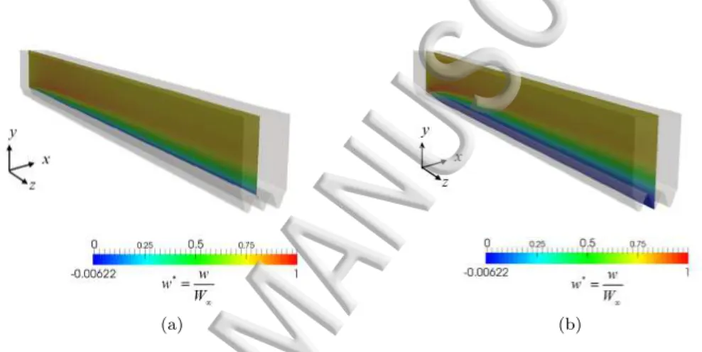
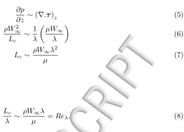
In contrast to the flat plate boundary layer, with a textured plate the velocity profile takes various shapes at each cross section depending on the span-wise (x-direction) location across the plate. As an example, the velocity profiles at 7 equi-spaced distances across a single sinusoidal wrinkle with AR = 1.91 at ReL= 13300 and L/λ = 47.75 are presented in Figure
4. Similar shaped velocity profiles have been previously reported in both experimental and numerical simulations by Djenidi et al.12,13 They reported velocity profiles, further away from the leading edge at a Reynolds number of ReL = 7.13× 10⁴ for a plate of L/λ = 92
featuring V-shaped grooves with AR = 1.72. Their profiles were comparable with the key features reported here, showing a retarded (nearly stagnant) flow inside the grooves (with a local velocity less than 20% of the free-stream velocity) while outside of the riblets all velocity profiles collapsed onto the same universal profile. Similar flow retardation and mean velocity profiles have been reported for turbulent flow over thin rectangular riblets as well as V-groove and U-groove textures of different sizes15,18,29.
Because the differences in the shape of the velocity profiles vary systematically with the cross sectional position (x), the velocity profiles at the peak (x = λ) and in the trough (x = λ/2) of the wrinkles are chosen as the representative profiles to be discussed further as they
(a) (b)
FIG. 4. (a) Contours of dimensionless velocity and (b) velocity profiles w(x, y)/W∞at 7 different locations of x = iλ/6 and 0≤ i ≤ 6, within a single groove of a wrinkled plate with AR = 1.91 and L/λ = 47.75 at ReL= 13300; Here η = y/L
√
ReLwhich is the same definition as used in the flat plate boundary layer theory. The dashed line denotes the theoretical profile from the Blasius solution to boundary layer equation for a flat plate (AR = 0).
(a) (b)
FIG. 5. Schematic of the evolution in the boundary layer at (a) the peak (x = λ , ymin= 0) and (b) the trough (x = λ/2 , ymin=−A) of a sinusoidal riblet surface with ReL= 13300, L/λ = 47.75 and AR = 1.91.
present the two extrema of the problem. To illustrate qualitatively the three-dimensional evolution in the flow, contours of the dimensionless velocity distribution (w/W∞) at the peak and trough for ribbed plates at ReL= 13300, L/λ = 47.75 and AR = 1.9 are shown in
Figures 5(a) and 5(b) respectively. Qualitatively the velocity contours at the peak appear very similar to the evolution observed along a flat plate boundary layer while the contour distribution in the trough differs from the peak and depict a thicker boundary layer for which most of the region inside the groove has velocities lower than 25% of the free-stream velocity.
The evolution in the velocity distributions can be studied more quantitatively by plotting the spatial changes of the velocity profiles in the flow direction, as shown in Figure 6. Here we non-dimensionalize the position along the plate using a characteristic diffusive scale ν/W∞ so that the dimensionless position corresponds to a local Reynolds number Rez= W∞z/ν. Although the wrinkles (sinusoidal riblets) result in different velocity profiles
at different locations, the main features and the local differences induced by the riblets can be effectively contrasted by comparing the velocity profiles at the peak and trough of a single riblet. Figures 6(a) and 6(b) present the velocity profiles at the peak and trough respectively (corresponding to the velocity contours in Figure 5). As we have noted, the stream-wise profiles at the peak, w(x = λ, y) closely resemble the profiles of flat plate boundary layer theory. In the trough, the profiles w(x = λ/2, y) look markedly different and reveal a thicker boundary layer, with the velocity inside the groove (y < 0) much lower than the free-stream velocity. For this case with AR = 1.91 the minimum velocity observed in each profile i.e. wmin = min(w(x = λ/2, y)) is not always zero (as it is for the velocity
(a)
(b)
FIG. 6. Evolution of stream-wise velocity profiles w(x, y, z) in the flow direction along (a) a peak x = λ and ymin= 0 and (b) along a trough x = λ/2 and ymin=−A of a surface with sinusoidal riblets with L/λ = 47.75 and AR = 1.91 at ReL= 13300.
profiles at the peak x = λ), but can in fact become negative and within a region between about 2500 < Rez< 10500, a local re-circulation is observed. The location of the minimum
velocity at each position z along the plate is shown in Figures 6(a) and 6(b) by the red circles joined by a line. If there is a re-circulation present, then the line of minimum velocity is displaced from the wall inside the groove. As a consequence above this line of points, a stagnation line is also formed inside the grooves and shown in each figure by the solid green line and triangular symbols.
At three representative local positions (corresponding to local Reynolds numbers of Rez=
4000, 8000 and 12000) velocity profiles are extracted and plotted as shown in Figures 7. For Rez = 4000 and Rez = 8000 the trough profiles show a region of weak re-circulation
inside the grooves (y < 0) whereas outside the groove, the velocity profiles at the peak and at the trough collapse on each other and evolve in similar fashion toward the outer inviscid flow far from the plate. Further along the plate at Rez = 12000, the recirculating region
ends, and thereafter the fluid inside the groove is in an essentially stagnant condition with zero velocity. Outside the groove the two velocity profiles meet and grow similarly to reach the free-stream velocity.
Our detailed computations of the velocity field in the vicinity of the sinusoidal texture reveal that due to the presence of the wrinkles the flow inside the grooves feels a strong retardation that ultimately results in this local re-circulating region. Eventually, as the frictional effects of the walls diffuse further outwards, the recirculating region ends and the fluid in the groove becomes almost stagnant inside the grooves. This stagnant fluid acts like a “cushion” of fluid on which the fluid outside of the grooves can slide. Similar behavior is
(a) (b) (c)
FIG. 7. Normalized velocity profiles at peak and trough at different locations (a)Rez = 4000, z/λ = 14.32 , (b)Rez= 8000, z/λ = 28.65 and (c)Rez= 12000, z/λ = 42.97 along the flow direction for a riblet surface with AR = 1.91 and L/λ = 47.75.
observed for cases with higher Reynolds numbers and longer lengths (achieved by changing the inlet velocity and the length of the plate). For example, for riblets of AR = 1.91 with global Reynolds number of ReL = 120600 and L/λ = 95.5, velocity profiles in the trough
are presented in Figure 8 and as it can be seen the re-circulation starts at a later position (i.e. a higher local Rez) and it extends to a larger distance downstream.
FIG. 8. Normalized velocity profiles along the flow direction in the trough of a wrinkle for ReL= 120600 , L/λ = 95.5 and AR = 1.91.
However, the aspect ratio AR of the wrinkles also has an effect on whether a re-circulating region is created or not. The progression of local velocity profiles for a wrinkled texture with global Reynolds number ReL = 13300 and L/λ = 47.75 with a lower aspect ratio of
AR = 0.95 (compared to AR = 1.91 in Figure 6(b)) is presented in Figure 9. Again we can see flow retardation inside the grooves with a stagnant layer of fluid and a bounding stagnation line, shown with a green line with triangular symbols. However for this shallower riblet geometry the minimum velocity is zero and located at the wall (shown by red line with circular symbols) and thus no re-circulation develops in the groove (y < 0).
This local re-circulation in the grooves can also be identified by using other vortex identi-fication methods such as the scalar measure Q defined as Q = Ω : Ω−S : S.21This measure based on the the second invariant of the velocity gradient tensor, compares the rotation rate in the fluid (the anti-symmetric part of the velocity gradient tensor Ω =1
2(∇u−∇u
T) ) with
the irrotational straining (symmetric part of the velocity gradient tensor S = 12(∇u+∇uT)) in the fluid.21. For example for Re
L = 13300 and L/λ = 47.75 the iso-Q surfaces of
Q = 1206.5 < ωz,w >2 are shown in Figure 10 where ωz is the z component of the vorticity
FIG. 9. Normalized velocity profiles along the flow direction in the trough of a wrinkle for ReL= 13300, L/λ = 47.75 and AR = 0.95.
the wall. The observed vortical structures develop in the same region within the grooves as the local flow re-circulation that was observed in Figure 6(b).
FIG. 10. Vortical structures in the grooves of a wrinkled surface for ReL= 13300, L/λ = 47.75 and AR = 1.91 revealed by an iso-Q surface with Q = 1206.5 < ωz,w>2; As seen in the figure the vortical structures are located in the middle of the re-circulating region identified in Figure 6(b).
Close to the leading edge of the plate, the effects of stream-wise pressure gradients are not negligible and this results in velocity profiles with a higher maximum velocity than the bulk fluid velocity Win at the inlet27,32. To evaluate the effects of this local acceleration near
the leading edge, the stream-wise pressure distribution above one of the troughs (x = λ/2) at y = 0 is shown in Figure 11. Figure 11(a) shows the dimensionless pressure distribution p∗ (scaled as p∗ = p/12ρW∞2) as a function of the local position along the plate (or local Reynolds number, Rez) for a series of different aspect ratio wrinkles, keeping the inlet
velocity constant. As seen in the figure, close to the leading edge a favorable pressure gradient (pressure decrease) is observed. However at an intermediate location along the plate this turns into an adverse pressure gradient (local stream-wise pressure increase) and ultimately the pressure increases to an asymptotic value of zero (set by the exit boundary condition).
In the case of the boundary layer over a flat plate (AR = 0), the changes in pressure disappear after Rez ≈ 15000, and from there onwards, the classical flat plate boundary
layer approximation of ∂P∂z ≈ 0 is a valid assumption to simplify the equations of motion. However, in the presence of the riblets, the region of favorable pressure gradient is extended and the pressure decreases to progressively lower values as the riblet aspect ratio increases. This results in the need for a larger pressure recovery in the adverse pressure gradient region, and this contributes to the establishment of local flow re-circulation. Comparing the case of AR = 1.91 from Figures 11(a) and 6(b) we can observe that the location of the minimum pressure is consistent with the location of the start of the re-circulation
textured plate does not exhibit any re-circulation in the grooves (cf. Figure 8). However, for aspect ratios of AR & 0.95 the magnitude of the local adverse pressure gradient is notably enhanced and the recirculating region shown in Figures 6(b) and 8 develops.
(a) (b)
FIG. 11. (a) Stream-wise pressure distribution at x = λ/2 and y = 0 (above a trough) as a function of the local Reynolds number down the plate for different aspect ratio riblets, keeping the inlet velocity constant (ReL= 25000 and L/λ = 95.5). Inset shows additional details for small values of Rez< 103on a logarithmic scale. (b) Pressure distribution along the direction of flow on top of a groove at y = 0 for various inlet velocities (and different global Reynolds numbers) and L/λ = 95.5.
The evolution of similar pressure distribution can be calculated for the case of AR = 1.91 and L/λ = 95.5, and different global Reynolds numbers of 2.5× 10⁴, 5.1× 10⁴ and 2.5× 10⁵ (by changing the inlet velocity) and are presented as a function of the position or local Reynolds number in Figure 11(b). Comparing the three cases shows that the location of the minimum pressure (which coincides with the start of the recirculating region in the case of AR = 1.91) evolves with changes in the inlet velocity while the magnitude of the minimum dimensionless pressure stays nearly constant. We denote the location of the minimum pressure as Lc and seek to find a scaling for Lc as the flow geometry changes.
Since the flow in the boundary layer close to the leading edge is quasi-steady and inertial pressure effects balance viscous stresses we expect that the pressure drop is of the same order as the divergence of the shear stress tensor in the z direction inside the grooves. A scaling estimate for the pressure gradient in this region gives
∂p ∂z ∼ ρW2 ∞ Lc (3)
and the divergence of the shear stress tensor in the z direction for the viscous flow inside the grooves (with characteristic groove length scale λ) can be expressed as
(∇.τ )z∼ 1 λ ( µW∞ λ ) . (4)
Therefore for the pressure gradient to balance with the shear stress gradient inside the grooves, we require
∂p ∂z ∼ (∇.τ )z (5) ρW∞2 Lc ∼ 1 λ ( µW∞ λ ) (6) Lc∼ ρW∞λ2 µ (7) or in dimensionless form Lc λ ∼ ρW∞λ µ = Reλ. (8)
Therefore, the location of the minimum pressure along the plate is expected to increase linearly with increases in the inlet velocity. Figure 12 shows the calculated location of the minimum pressure for cases with inlet velocities 0.5≤ Win ≤ 7 m/s (and calculated
maximum velocities of 0.6 ≤ W∞ ≤ 8.2 m/s, respectively) for wrinkles with AR = 1.91 plotted as a function of ρW∞λ/µ. It can be seen from the figure that the calculated location scales linearly with the Reynolds number based on the wrinkle length scale (λ) Reλ = ρW∞λ/µ as predicted using the scaling above. Additional computations indicate
that keeping the inlet velocity constant and varying the wavelength at a constant aspect ratio of AR = 1.9 results in the same scaling as Equation 8 and in Figure 12.
FIG. 12. Location of the minimum pressure for flow over textured surfaces with various inlet velocities 0.5 ≤ Win ≤ 7 m/s and the calculated maximum velocities of 0.6 ≤ W∞ ≤ 8.2 for AR = 1.91.
A principal goal of the present study is to investigate the source of friction reduction arising from variations in the texture of the surface. The local shear stress acting on the surface is directly proportional to the velocity gradient at the wall. Furthermore, as was seen earlier, the presence of the wrinkled topography provides a method to alter the curvature of the velocity profiles near the plate, especially inside the grooves, thus resulting in lower velocity gradients at the walls (for example, compare the peak and trough profiles in Figures 7). This results in a lower local wall shear stress inside the grooves compared with an equivalent flat plate and thus can result in a net reduction in the local average shear stress. This is especially seen in the recirculating region and stagnant areas where there is a cushion of almost stationary fluid. In these regions the velocity gradient is small or close to zero (as seen in Figure 6(b)). However, conversely, the total surface area of a grooved or ridged surface over which the shear stress is acting increases with the ridge scales and this can potentially offset or even overwhelm the local friction reduction. We therefore now proceed to carefully evaluate each contribution to the total skin friction on a wrinkled surface.
∆∗ z αλ = 1 z αλ ∫ S ( 1− w W∞ ) dS (9)
where ∆∗is now a displacement area, α is the number of wrinkles modelled in the simulation, z is the local stream-wise location and S is the cross sectional area of the flow in the x− y plane. This expression for ∆∗(z) is defined locally but the equation can be extended to a global definition by replacing the position z with the total plate length L. The boundary layer thickness for a flat plate (AR = 0) and three different wrinkle textures of AR = 0.48, AR = 0.95 and AR = 1.91 are calculated for cases with various inlet velocities and a fixed L/λ = 47.75 and plotted on double logarithmic axes versus the global Reynolds number ReL= ρW∞L/µ in Figure 13. From the figure, it is clearly seen that increasing the aspect
ratio of the riblets (AR) results in an increase in the thickness of the boundary layer, as expected from the velocity contours shown in figure 6.
At higher Reynolds numbers ReL > 104 when the initial pressure gradient is negligible,
the flat plate results extracted from the computations follow the Re−0.5L scaling as calculated by Blasius. However, for lower Reynolds numbers, where the effects of the initial pressure gradient are non-negligible along the entire length of the plate, the data follows the scaling found from the higher order boundary layer theory results presented by van de Vooren and Dijkstra36, which can be fitted to a power law proportional to Re−0.44
L .
FIG. 13. Boundary layer thickness for different ReL and different wrinkle aspect ratios; in all cases L/λ = 47.75 and for each profile the change in the Reynolds number is due to systematically changing the inlet velocity Winwhich results in changes of the calculated maximum velocity W∞. In addition to the displacement area, a momentum area (the equivalent of the classical momentum thickness for a boundary layer that now varies in both x and y) can be calculated using the following expression14,32
Θ z αλ = 1 z αλ ∫ S w W∞ ( 1− w W∞ ) dS. (10)
Similar to displacement area, the above definition is local and it can be extended to a global definition by replacing the position z with the length of the plate L.
Keeping the inlet velocity constant, the variation of the displacement area (∆∗) and mo-mentum area (Θ) locally along the flow direction (z) are plotted in Figure 14 for wrinkles
with various aspect ratios, showing an increase in the local displacement area of the bound-ary layer as AR increases. For all wrinkled cases studied this value is larger than for a flat plate with AR = 0 but the results slowly converge as Rez increases beyond 104. This
provides a clear indication that the effects of the wrinkled texture on the boundary layer size decay away as the flow progresses along the plate. In the case of the momentum area, again the local value of the momentum area for wrinkled walls is always larger than the flat wall, but as Rez increases beyond 104, the data once again converges to the flat plate
results.
(a) (b)
FIG. 14. Evolution of (a) the local displacement area (∆∗) and (b) the local momentum area (Θ) along the plate (plotted in the form of a local Reynolds number Rez) for wrinkles with different aspect ratios 0 < AR < 2 keeping the length (L/λ = 191) and inlet velocity constant Win= 1 m/s. For these conditions, calculations for a flat plate (AR = 0) give W∞= 1.33 m/s.
The shape factor H = ∆∗/Θ, is used frequently in aerodynamics as an indicator of boundary layer separation and re-circulation5,14,32. For flow over a flat plate in the laminar regime, H < 2.65 and at higher Reynolds numbers it reaches the value of H = 2.65 as given by the Blasius solution. The shape factor of the evolving boundary layer profiles along the length of the plates are shown in Figure 15 for wrinkles with different aspect ratios as a function of the local Reynolds number Rez (corresponding to Figure 14). The
introduction of stream-wise wrinkles results in an increase in the local shape factor of the viscous boundary layer and as the aspect ratio of the wrinkles progressively increases the shape factor H increases. This indicates a retardation in the local velocity close to the wall compared with the flat wall (H < 4)14, but no re-circulation for 0 < AR < 1.5. For the case with the highest aspect ratio (AR = 1.91), the shape factor reaches a peak value of H = 4.5 at Rez∼ 4000 and then as the flow progresses along the plate H monotonically decays to
a nearly constant value. The region with local Reynolds number of 3000 6 Rez 6 8000
where the shape factor goes through an increase and then a decrease corresponds to the re-circulation region documented earlier in Figure 6(b). At distances further down the plate the amplified value of the shape factor (H > 2.65) is a quantitative indication of fluid flowing over a cushion of stagnant fluid.
It is of interest to understand the differences between the calculated velocity profiles obtained for flow over wrinkled surfaces with different aspect ratios and the corresponding Blasius solution for the flat plate at every location of the riblet cross section. As we saw earlier, far from the surface of the riblets, the velocity profiles at different cross sectional locations collapse onto the same profile and behave similarly to the Blasius solution (Figure 4). Additionally, as we move further down the plate, the effects of the riblets on the velocity profile are confined to the creation of a cushion of stagnant fluid inside the grooves and are barely noticeable outside the grooves. In order to examine the difference between the classical two dimensional boundary layer and the current computations, the velocity contours at each cross section are decomposed into two additive contributions; the first contribution assumes the flat plate boundary layer solution of Blasius holds at every location in the cross section and is here denoted by wBL(x, y). The second contribution is obtained from the difference between the actual velocity profile w(x, y) and the flat plate boundary
FIG. 15. Shape factor (H = ∆∗/Θ) of the velocity profile in a viscous boundary layer for different aspect ratio wrinkles corresponding to Figure 14.
layer solution at every cross sectional location, denoted by ∆w(x, y) = w(x, y)− wBL(x, y); therefore: w(x, y) W∞ = wBL(x, y) W∞ + ∆w(x, y) W∞ . (11)
The velocity gradient and the shear stress (proportional to the velocity gradient at the wall or n = 0) can thus also be decomposed into two parts:
∂w ∂n = ∂wBL ∂n + ∂∆w ∂n → τ = τBL+ µ ∂∆w ∂n (12)
where τBL is the wall shear stress on the wrinkled wall, assuming the flat plate boundary layer solution holds at every location. This decomposition can be used to understand the increase or reduction in the local shear stress due to the periodic texture of the wall and illustrative examples of this decomposition are presented in Figures 16, 17 and 18. If the flat plate solution was the solution everywhere to the velocity field (wBL), then the gradient
of the velocity field normal to the wall (n) evaluated at the wall (n = 0 or y = ys) could be
found from the expression
∂wBL ∂n n=0 = √ 1 +(πAλ sin(2πλx))2 ∂wBL,f ∂y y=ys (13)
where wBL,f is the Blasius solution on the flat plate. The shear stress at the wall is defined as τ = µ ∂w/∂n|n=0, thus
τBL= √
1 +(πAλ sin(2πλx))2 τBL,f (14) where τBL,f is the wall shear stress for the flat wall as calculated by the Blasius solution. Since the first trigonometric term in the expression in Equation 14 is always larger than or equal to unity, the shear stress at the wall of a textured surface (in this case a sinusoidally wrinkled surface) would be higher than that of the flat plate if the Blasius solution were to hold everywhere for flow over a riblet surfaces (τBL > τBL,f). Therefore, any local decrease in the shear stress on the wrinkled plate (compared with the flat plate) will be dependent on the sign of the last term in Equation 12. This decomposition can be used to explain how wrinkle size affects changes in the viscous shear stress compared to the stress distribution above a flat plate at the same local Reynolds number Rez. For example the cross sectional
(a) (b) (c)
FIG. 16. Decomposition of the full computed velocity profile (w/W∞) shown in (a) into two pieces; the first one shown in (b) is based on the flat plate boundary layer wBL/W∞plus a velocity defect (∆w/W∞) shown in (c). Figures above shown for Rez= 4000 and z/λ = 14.32 with AR = 0.48.
(a) (b) (c)
FIG. 17. Decomposition of the full computed velocity profile (w/W∞) shown in (a) into two pieces; the first one shown in (b) is based on the flat plate boundary layer wBL/W∞plus a velocity defect
(∆w/W∞) shown in (c). Figures above are for Rez= 4000 and z/λ = 14.32 with AR = 0.95.
(a)w/W∞ (b)wBL/W∞ (c)∆w/W∞
FIG. 18. Decomposition of the full computed velocity profile (w/W∞) shown in (a) into two pieces; the first one shown in (b) is based on the flat plate boundary layer wBL/W∞plus a velocity defect
(∆w/W∞) shown in (c). Figures above are for Rez= 4000 and z/λ = 14.32 with AR = 1.91.
velocity contours for three different wrinkle sizes (AR = 0.48, AR = 0.95 and AR = 1.91) with Rez = 4000 and z/λ = 14.32 are shown in Figures 16, 17 and 18. In each case the
wrinkles have the same wavelength while only the amplitude of the wrinkles is changed. In all the figures, the y direction is normalized with the constant wavelength (λ) of the wrinkle. The most prominent differences between the actual velocity profiles shown in Figures 16(a), 17(a) and 18(a) and the locally-shifted form of the Blasius solution wBL (Figures
16(b), 17(b) and 18(b)) is inside the grooves where the velocity boundary layer is thicker and the flow is almost stagnant close to the wall (as was also demonstrated earlier). There-fore, the velocity defect ∆w (shown in Figures 16(c), 17(c) and 18(c)) shows non-zero and negative values which results in a lower velocity gradient in the grooves compared with ∂wBL/∂n|n=0inside the grooves. Another region of difference is at the peak of the riblets. Here the difference is not as clearly discernible, but is clearly non-zero and yields posi-tive values of the velocity defect ∆w (with magnitudes lower than those observed inside the grooves). This results in a slightly higher velocity gradient at the peak of the riblets
result in an increase in the wall shear stress calculated by using just the Blasius solution for the riblets (τBL) without correction. However when examining the actual velocity defect
structure in Figures 17(c), 16(c), and 18(c) we see a stronger negative velocity gradient inside the grooves which, from Equation 12, can result in a reduction in the net local shear stress evaluated at each cross section along the plate.
C. Wall Shear Stress and Drag
Finally, we investigate the ability of the riblets to reduce the total drag force exerted on the wall. To do this we evaluate the average skin friction coefficient Cf (Figure 19(a)) and
the total integrated drag force D (Figure 19(b)) with respect to the flat surface. We consider cases with different aspect ratios (0 < AR < 2) and constant L/λ = 47.75, as a function of the global Reynolds number ReL (by using different inlet velocities Win and computing
the maximum calculated velocity W∞) for each case. If the stress tensor at the wall and local wall normal vector evaluated at a position xs, ys on the riblet surface are defined as
τw(xs, ys; z) and nw(xs, ys; z) respectively (where ys=−A2 +A2 cos(2πλxs)), then the total
drag force on a plate of length L and the average skin friction coefficient are defined as
D = ∫ L 0 [ τw(xs, ys; z).nw(xs, ys; z) ] .ez dAw (15) and Cf = D 1 2ρW∞2 Aw (16)
respectively, where Awis the wetted area of the riblet wall. A reduction in the skin friction
coefficient is defined as ∆Cf = Cf− Cf,0 where Cf,0is the skin friction coefficient of a flat
plate and the reduction in total drag is defined as ∆D = D− D0 where D0 is the total drag on the flat surface. Note that negative values in both plots correspond to skin friction coefficient reduction and drag reduction respectively. The results in Figure 19 show that the presence of the riblets reduces the average skin friction coefficient on the wall in nearly all of the riblet cases considered. At the same value of the global Reynolds number (ReL)
increasing the aspect ratio (AR) results in a progressively larger decrease in the average skin friction coefficient. This also confirms our observations based on consideration of the velocity decomposition that the negative velocity defect observed inside the grooves (Figures 16(c), 17(c) and 18(c)) results in a reduction in the average shear stress compared to the flat plate. As the aspect ratio of the wrinkles increases, the increase in the magnitude of the negative velocity defect ∆w < 0 results in a higher reduction in the average skin friction coefficient.
However, reduction of the average skin friction coefficient alone cannot define whether a textured riblet surface is drag reducing or not because the total area of the wetted surface is also increased through the presence of the wrinkles. The total wetted surface area of the textured plate is larger than a flat surface and increases with AR; thus for a textured surface to be drag reducing the reduction in the skin friction coefficient due to the riblets must more than offset the increasing wetted area. For the results shown in Figure 19(b) at L/λ = 47.75 the only cases that appear to show a net drag reduction are the cases with aspect ratios of AR = 0.48 and AR = 0.95 and global Reynolds number of ReL = 13300.
(a)
AB
C
(b)
FIG. 19. Reduction in (a) the skin friction coefficient (Cf) and (b) changes in the total drag (D) for wrinkles of different aspect ratios, fixed plate length L/λ = 47.75 and different ReL (varying the inlet velocity). Points A, B and C correspond to the same points shown below in Figure 21(b).
The rest of the cases show substantial increase in the total drag when compared to an equivalent flat surface.
To better understand these drag reducing cases and how changes in the length of the plate (ReL) and aspect ratio (AR) interact to affect the total drag, we consider the following
situations: we keep the inlet velocity constant (thus keeping W∞constant) and extend our calculations to plates of longer total lengths than those used in the computations presented in Figure 19. We consider a maximum plate length of L/λ = 191 and an inlet velocity of Win= 1 m/s (thus corresponding to a maximum global Reynolds number of ReL= 5×10⁴)
for 5 different aspect ratios of 0 < AR < 2. The results are shown in Figure 20. We first consider the distribution of the wall shear stress on the wall as a function of different aspect ratios at different positions z along the length of the plate corresponding to different values of the local Reynolds number, Rez. From steady two-dimensional boundary layer theory
we know that the local shear stress on the wall decreases along the plate as τBL∼ Re−1/2z
(Equation 2). For reference we therefore plot this result as the black dashed line in Figure 20(a). For a ribbed plate, the wall shear stress is now a function of lateral position xs, ys
on the surface as well as distance down the plate. We therefore define the dimensionless local average shear stress distribution at any distance z along the plate as
τ∗(z) = 1 1 2ρW∞2 1 lC ∫ C τw(xs, ys; z).nw(xs, ys; z).ezdl (17)
where C is the riblet contour at each stream-wise cross section, lC is the total length of the
riblet contour (lC =
∫
Cdl) and dl is the line element along the rib transverse to the flow
direction. In Figure 20(a) we show the evolution in the local average shear stress along the length of the plate for wrinkled cases with 0 < AR < 2 and plates with ReL= 4× 10⁴ and
L/λ = 191 compared with the shear stress on the flat plate. It is clear that the presence of the wrinkles changes the evolution in the shear stress distribution along the flow direction. As seen in this figure, close to the leading edge of the plate, the presence of wrinkles does not reduce the large initial shear stress that results from the sudden generation of vorticity at the leading edge. However as the local Reynolds number Rez increases along the plate,
the wrinkles retard the flow in the grooves and thus reduce the local average shear stress at the wall. The case of AR = 1.91 shows a region with almost constant average shear stress between 5000 < Rez < 12000 which also corresponds with the re-circulation region
presented earlier in Figure 6(b). Smaller aspect ratios do not show any re-circulation and thus there is no region with constant shear stress distribution.
At lower local Reynolds numbers Rez6 103(close to the leading edge), the local average
shear stress for all the riblet cases is nearly the same as the shear stress distribution on the flat plate. However, as we established above, increasing the aspect ratio of the riblets
(a) (b)
FIG. 20. (a) Evolution of the local transverse average of dimensionless wall shear stress distribution (Equation 17) for the same inlet velocity and different aspect ratio riblets. (b) Increases (∆D > 0) and reductions (∆D < 0) in the total drag force (D) for wrinkled plates of different total length of the range 0 < L/λ < 191 (increasing global Reynolds number ReL) for various aspect ratio wrinkles 0 < AR < 2, keeping the wavelength λ constant.
results in an increase in the wetted area and therefore this results in a substantial increase in the total drag for plates with AR > 0.48 and global Reynolds numbers of ReL < 8000
(and nearly no change in the total drag for the case of AR = 0.48). However, further down the plate, as the cushion of stagnant fluid starts to form inside the grooves, the reduction in the local shear stress can offset the increase in the wetted area and this results in a net reduction of the total drag.
As we show in Figure 20(b) it becomes clear that riblets have the potential of reducing drag provided the plate is longer than a minimum critical length ReL,c(AR) (which can
be determined from where each of the curves cross the value of zero on the ordinate axis). Secondly, the sharpness of the riblets plays an important role in controlling the extent of total drag reduction achieved. Higher aspect ratio wrinkles provide greater local shear stress reduction but this is offset by the large increase in wetted area for very high aspect ratios. For the range of global Reynolds number ReL we have studied, the case with AR = 0.95
was found to provide the highest reduction in the total drag. We can illustrate this most clearly by holding the global Reynolds number ReL and riblet spacing L/λ constant and
calculating the total drag reduction as a function of the aspect ratio of the riblets. We illustrate this in Figure 21(a) for three different values of ReL showing that for each of the
cases there is an optimum aspect ratio providing the largest possible drag reduction. Quite generally we find that the total frictional drag reduction (corresponding to ∆D/D0< 0) at a constant global Reynolds number ReLand L/λ is first enhanced as the aspect ratio of the
wrinkles increases, then reaches an optimum and as the aspect ratio increases still further the extent of drag reduction decreases and eventually shifts to a net drag increase. For ReL> 104the optimum aspect ratio is slightly less than unity, but after that the optimum
aspect ratio is close to AR≈ 1. Previous wind tunnel experiments by Walsh with V-groove riblets of AR = 1 and AR = 2 at constant free-stream velocity also show that riblets with AR = 1 result in a larger drag reduction compared to AR = 2.39
A similar trend as discussed above can be observed for the other data points presented in Figure 19(b) as the plate length is increased. To illustrate that, at a constant aspect ratio of AR = 1.9 (which did not show any drag reduction for the case of L/λ = 47.75) the evolution in the total drag force for plates of various lengths (1 < L/λ < 191) with different inlet velocities are presented in Figure 21(b). As we discussed in section III A, changing the inlet velocity results in a change in the pressure distribution (Figure 11(b)) and thus alters the location of the minimum pressure inside the grooves (Figure 12). For short plates, the presence of the wrinkles leads to an overall increase in the frictional drag, but in each case a net drag reduction is observed when the length of the plate exceeds a critical value. However, due to the differences in the pressure distribution among the cases with different inlet velocities, the cross over from drag increase to drag decrease occurs at
(a)
A B
C
(b)
FIG. 21. (a) Drag reduction curve for plates with global Reynolds number of ReL= 15000 and plate length L/λ = 58.82, global Reynolds number ReL= 30000 and plate length L/λ = 117.64, and global Reynolds number ReL = 45000 and plate length L/λ = 176.46 (same inlet velocity Win = 1 m/s and the same wavelength λ = 2π/3× 10−1 mm) as a function of the aspect ratio of the riblets. (b) Reduction in total drag for wrinkled plates of different length ReL, AR = 1.9 and inlet velocities of Win= 1, 2 and 5 m/s corresponding to Reλ= 278.55, 534.07 and 1256.64. Points A, B and C correspond to the same points in Figure 19(b).
a longer plate length as the free-stream velocity (and thus Reλ) is increased. Points A, B
and C indicated on the figure correspond to the points A, B and C noted in figure 19(b) (ReL = 1× 10⁴, 2.4× 10⁴, and 5.9× 10⁴ respectively) where for a fixed plate length of
L/λ = 47.75 only a net drag increase was observed.
IV. CONCLUSIONS
In this paper we have examined in detail the effects of sinusoidal riblets on the structure and evolution of a steady viscous boundary layer. The presence of the riblets results in a local flow retardation inside the valleys of the riblets and even the possibility of a local flow reversal. Riblets increase the average thickness of the boundary layer as well, resulting in an increase in the shape factor of the boundary layer. The presence of riblets also change the pressure distribution close to the leading edge of the plate when compared with the flat boundary layer. This flow retardation creates a cushion of almost stagnant fluid inside the riblets upon which the fluid flowing above the plate can slide. This creates a non-uniform shear stress distribution laterally across the plate and a local average shear stress lower than the corresponding flat plate. For sufficiently long plates, this can result in a reduction of the total viscous drag force acting on the surface compared with flat surfaces, provided the aspect ratio of the wrinkles is not so large that the increase in wetted area offsets the local reduction in wall shear stress τw(xs, ys). By careful computation of the local skin friction
coefficient Cf(xs, ys) as well as the total integrated frictional drag force D we have shown
that the reduction in drag is a function of the aspect ratio of the riblets. For each ReL and
L/λ there is an optimum aspect ratio where the highest drag reduction can be achieved. For fully developed viscous boundary layers at ReL& 104 (so that leading edge effects are not
important), it appears that aspect ratios of order unity produce the maximum reduction in drag, which can be as large as ∆D/D0≈ −20% at ReL≈ 4 × 10⁴.
These detailed computations help rationalize why previous experimental measurements have reported conflicting conclusions regarding drag increases or decreases and will pro-vide guidance for selecting optimal riblet sizes and spacings for specific design applications requiring minimized frictional drag.
of shark skin,” Experiments in Fluids 28, 403–412 (2000).
3Bechert, D., Bruse, M., Hage, W., Van der Hoeven, J. T., and Hoppe, G., “Experiments on
drag-reducing surfaces and their optimization with an adjustable geometry,” Journal of Fluid Mechanics 338, 59–87 (1997).
4Bechert, D., Hoppe, G., and Reif, W.-E., “On the drag reduction of the shark skin,” in 1985 AIAA Shear
Flow Control Conference (1985).
5Blackwell, J. A., “Preliminary study of effects of reynolds number and boundary-layer transition location
on shock-induced separation,” NASA-TN-D-5003 (1969).
6Chan, E. P., Smith, E. J., Hayward, R. C., and Crosby, A. J., “Surface wrinkles for smart adhesion,”
Advanced Materials 20, 711716 (2008).
7Chen, X. and Hutchinson, J. W., “Herringbone buckling patterns of compressed thin films on compliant
substrates,” Journal of Applied Mechanics 71, 597 (2004).
8Choi, H., Moin, P., and Kim, J., “Direct numerical simulation of turbulent flow over riblets,” Journal of
Fluid Mechanics 255, 503–539 (1993).
9Choi, K., Gadd, G., Pearcey, H., Savill, A., and Svensson, S., “Tests of drag-reducing polymer coated on
a riblet surface,” Applied Scientific Research 46, 209–216 (1989).
10Chu, D. C. and Karniadakis, G. E., “A direct numerical simulation of laminar and turbulent flow over
riblet-mounted surfaces,” Journal of Fluid Mechanics 250, 1–42 (1993).
11Dinkelacker, A., Nitschke-Kowsky, P., and Reif, W.-E., “On the possibility of drag reduction with the
help of longitudinal ridges in the walls,” in Turbulence Management and Relaminarisation (Springer, 1988) pp. 109–120.
12Djenidi, L., Liandrat, J., Anselmet, F., and Fulachier, L., “Numerical and experimental investigation of
the laminar boundary layer over riblets,” Applied Scientific Research 46, 263–270 (1989).
13Djenidi, L., Squire, L., and Savill, A., “High resolution conformal mesh computations for V, U or L groove
riblets in laminar and turbulent boundary layers,” in Recent Developments in Turbulence Management (Springer, 1991) pp. 65–92.
14Drela, M., Flight vehicle aerodynamics (MIT Press, 2014).
15El-Samni, O., Chun, H., and Yoon, H., “Drag reduction of turbulent flow over thin rectangular riblets,”
International Journal of Engineering Science 45, 436–454 (2007).
16Ferziger, J. H. and Peric, M., Computational Methods for Fluid Dynamics (Springer Science & Business
Media, 2012).
17Furuya, Y., Nakamura, I., Miyata, M., and Yama, Y., “Turbulent boundary-layer along a streamwise bar
of a rectangular cross section placed on a flat plate,” Bulletin of JSME 20, 315322 (1977).
18Goldstein, D., Handler, R., and Sirovich, L., “Direct numerical simulation of turbulent flow over a
modeled riblet covered surface,” Journal of Fluid Mechanics 302, 333–376 (1995).
19Hager, W., “Blasius: A life in research and education,” Experiments in Fluids 34, 566–571 (2003). 20Hooshmand, D., Youngs, R., Wallace, J., and Balint, J., “An experimental study of changes in the
structure of a turbulent boundary layer due to surface geometry changes,” in AlAA 21st Aerospace
Sciences Meeting, 83-0230 (American Institute of Aeronautics and Astronautics, 1983).
21Hunt, J. C., Wray, A. A., and Moin, P., “Eddies, streams, and convergence zones in turbulent flows,”
Studying Turbulence Using Numerical Simulation Databases-I1 , 193 (1988).
22Kennedy, J. F., Hsu, S.-T., and Lin, J.-T., “Turbulent flows past boundaries with small streamwise fins,”
Journal of the Hydraulics Division 99 (1973).
23Khan, M., “A numerical investigation of the drag reduction by riblet-surfaces,” in 4th Joint Fluid
Me-chanics, Plasma Dynamics and Lasers Conference, 86-1127 (AIAA, 1986).
24Kim, H., Kline, S., and Reynolds, W., “The production of turbulence near a smooth wall in a turbulent
boundary layer,” Journal of Fluid Mechanics 50, 133 (1971).
25Kim, J., Moin, P., and Moser, R., “Turbulence statistics in fully developed channel flow at low Reynolds
number,” Journal of Fluid Mechanics 177, 133166 (1987).
26Lee, S.-J. and Lee, S.-H., “Flow field analysis of a turbulent boundary layer over a riblet surface,”
Experiments in Fluids 30 (2001), 10.1007/s003480000150.
27Narasimha, R. and Prasad, S., “Leading edge shape for flat plate boundary layer studies,” Experiments
in fluids 17, 358–360 (1994).
28Neumann, D. and Dinkelacker, A., “Drag measurements on V-grooved surfaces on a body of revolution
in axial flow,” Applied Scientific Research (1991), 10.1007/BF01998668.
29Park, S.-R. and Wallace, J. M., “Flow alteration and drag reduction by riblets in a turbulent boundary
layer,” AIAA Journal 32, 31–38 (1994).
30Patankar, S. V. and Spalding, D. B., “A calculation procedure for heat, mass and momentum transfer
in three-dimensional parabolic flows,” International Journal of Heat and Mass Transfer 15, 1787–1806 (1972).
31Raayai-Ardakani, S., Yague, J. L., Gleason, K. K., and Boyce, M. C., “Mechanics of graded wrinkling,”
Journal of Applied Mechanics 83 (2016), 10.1115/1.4034829.
32Schlichting, H., Gersten, K., and Gersten, K., Boundary-layer theory (Springer, 2000).
33Simpson, R. L., An investigation of the spatial structure of the viscous sublayer (Max-Planck-Institut f¨ur
Str¨omungsforschung, 1976).
34Tardu, S. F., “Coherent structures and riblets,” Applied Scientific Research 54, 349385 (1995).
35Terwagne, D., Brojan, M., and Reis, P., “Smart morphable surfaces for aerodynamic drag control,”
Advanced Materials 26, 66086611 (2014).
36Van De Vooren, A. and Dijkstra, D., “The Navier-Stokes solution for laminar flow past a semi-infinite
flat plate,” Journal of Engineering Mathematics 4, 9–27 (1970).
37Versteeg, H. and Malalasekera, W., An Introduction to Computational Fluid Dynamics (Pearson, 1995). 38Viswanath, P., “Aircraft viscous drag reduction using riblets,” Progress in Aerospace Sciences 38, 571600
(2002).
39Walsh, M., “Drag characteristics of V-groove and transverse curvature riblits,” in Symposium on Viscous
flow drag reduction (AIAA Prog. Astronaut. Aeronaut., 1980).
40Walsh, M. and Lindemann, A., “Optimization and application of riblets for turbulent drag reduction,” in
22nd Aerospace Sciences Meeting (American Institute of Aeronautics and Astronautics, 1984) p. 347.
41Walsh, M. J., “Riblets as a viscous drag reduction technique,” AIAA journal 21, 485–486 (1983). 42Walsh, M. J., Viscous drag reduction in boundary layers, edited by D. M. Bushnell, Vol. 1 (AIAA, 1990)
Chap. Riblets, pp. 203–261.
43Walsh, M. J. and Weinstein, L., “Drag and heat-transfer characteristics of small longitudinally ribbed
surfaces,” AIAA Journal 17, 770771 (1979).
44Wen, L., Weaver, J., and Lauder, G., “Biomimetic shark skin: design, fabrication and hydrodynamic
function,” The Journal of Experimental Biology 217, 16561666 (2014).
45Yin, J., Yage, J. L., Eggenspieler, D., Gleason, K. K., and Boyce, M. C., “Deterministic order in surface