RLE Technical Report No. 520
June 1986
Robert A. Ulichney
Research Laboratory of Electronics Massachusetts Institute of Technology
Cambridge, MA 02139 USA
This work has been supported by the Digital Equipment Corporation.
L ·
P
It
on April 10, 1986 in partial fulfillment of the requirements for the degree of Doctor of Philosophy.
Abstract
Digital halftoning, also referred to as spatial dithering, is the method of render-ing the illusion of continuous-tone pictures on displays that are capable of only producing binary picture elements. This report addresses the problem of de-veloping such algorithms that best match the specific parameters of any target display device, modeled as the Physical Reconstruction Function, particularly for nonstandard grid geometries. Techniques are organized by computational complexity and according to the nature of the dots produced, dispersed or clus-tered. The point process of dispersed-dot ordered dither is generalized for both rectangular and hexagonal grids, by means of the Method of Recursive Tessella-tion, a sub-tiling algorithm. Hexagonal ordered dither proves to be the solution for asymmetric rectangular grids. The concept of blue noise-high frequency white noise-is introduced and found to have desirable properties for halftoning. Very efficient algorithms for dithering with blue noise are developed, based on perturbed error diffusion. The nature of dither patterns produced is extensively examined in the frequency domain. New metrics for analyzing the frequency content of periodic and aperiodic patterns for both rectangular and hexagonal grids are developed. Generalized sampling grids are also examined in detail; presented is a new "aspect ratio immunity" argument in favor of hexagonal grids. While some techniques benefit from the use of hexagonal grids, others are found to be ideally suited for rectangular grids. Several carefully selected digitally produced examples are included.
Name and Title of Thesis Supervisor: William F. Schreiber Professor of Electrical Engineering
-A:
r
1 ·
S.B., University of Dayton (1976)
S.M., Massachusetts Institute of Technology (1979)
E.E., Massachusetts Institute of Technology (1984)
Submitted to the Department of Electrical Engineering and Computer Science
in Partial Fulfillment of the Requirements for the Degree of
DOCTOR OF PHILOSOPHY
at the
MASSACHUSETTS INSTITUTE OF TECHNOLOGY June, 1986
(Robert A. Ulichney, 1986
The author hereby grants to M.I.T. permission to reproduce and to distribute copies of this thesis document in whole or in part.
Signature of Author ... . ...
Department of Electrical Engineering and 'omputer Science April 10, 1986 Certified by Accepted by William F. Schreiber Thesis Supervisor ,..o...o...o... Arther C. Smith Chairman, Departmental Committee on Graduate Students
·---t0
dl I
1.1 Choice of Halftone Techniques. 1.2 Image Rendering Systems . . . 1.3 Image Presentation Strategy .
1.3.1 Tone Scale Adjustment
2 Physical Reconstruction Functioi
2.1 Grid Geometries ...
2.1.1 Periodic Sampling Grids 2.1.2 Semi-Regular Grids
2.1.2.1 Effect of Aspect 2.2 Dot Function and Tone Map 2.3 Reflectance and Luminance
2.3.1 Direct Measurement . . . . . . . Ratio . . . . . . .. . . ..
3 Tools for Fourier Analysis
3.1 Periodic (Ordered) Patterns ...
3.1.1 Continuous-space Fourier Transform Computation . . . 3.1.2 Composite Fourier Transform ...
5 18 23 27 28 33 37 37 40 41 47 56 57 61 62 64 71 ~_ w ·_ __1_ -- -C·_ I_ .- IIC Z-- -... ... ... ... ... ... ... ... ... ... ...
3.2 Aperiodic Patterns ...
3.2.1 Estimating the Power Spectrum ...
3.2.2 Radially Averaged Power Spectra and Anisotropy 3.2.2.1 Quality of Measurement ...
4 Dithering with White Noise
4.1 Rectangular Grids ... 4.1.1 The Mezzotint .... 4.2 Hexagonal Grids ...
5 Clustered-Dot Ordered Dither
5.1 The Classical Screen ... 5.1.1 Orientation Sensitivity. 5.2 Rectangular Grids ...
5.2.1 Classical Screen at 45°... 5.2.2 Classical Screen at 0°... 5.2.3 The Spiral and Line Screens ... 5.2.4 Asymmetric Correction ... 5.3 Hexagonal Grids ...
5.3.1 Hexagonal Version of the Classical Screen 5.3.2 Spiral Screen ...
6 Dispersed-Dot Ordered Dither
6.1 Method of Recursive Tessellation ...
6.1.1 Tessellating Regular Grids . . . . 6.1.2 Generation of Threshold Arrays ... 6.2 Examples for Regular Grids ...
6.3 Exposure Plots ... 99 ... 100 ... ... 101 ... .. 108 ... .. 108 ... .. 123 ... .. 128 ... .. 136 ... .. 142 ... .. 142 ... ... 148 153 154 154 157 169 197 6 75 75 76 82 85 86 90 95 I ... ... ... . . . . . . . . . . . . . . . . . . . .
7.2 Rectangular Grid Solution ... 7.3. Examples for a, = 1 7.4 Examples for a, 6 ... 7.5 Crossover Points ... 7.5.1 Examples for a, = 1. 7.5.2 Examples for a, = 7.6 Summary ...
8 Dithering with Blue Noise
8.1 Principal Wavelength . ... 8.2 The Error Diffusion Algorithm ...
8.2.1 The Floyd and Steinberg Filter . . 8.2.2 Filters with 12 Weights.
8.3 Error Diffusion with Perturbation ... 8.3.1 One Weight ...
8.3.2 Two Weights ... 8.3.3 Four Weights ...
8.3.4 Asymmetric Robustness ... 8.4 Hexagonal Case ...
8.4.1 Error Diffusion with Perturbation
267 ... . . . 268 ... . . . 274 ... . . . 277 ... . . . 289 ... . . . 302 ... . . . 307 ... . . . 318 ... . . . 332 ... . . . 346 ... . . . 349 ... . . . 359 9 Concluding Remarks
9.1 Other Neighborhood Processes
373 . 373 7 .... 230 .... 240 .... 251 ... . 251 .... 256 .... 266 _·_ __·__1_11··_111___C· ... ... ... ... ... ...
9.1.1 Sharpening ... 374
9.2 Blue Noise is Pleasant ... 379
9.3 Beyond Binary Displays ... 382
9.4 Suggestions for Future Research . ... 385
9.5 Summary ... 387
Glossary of Principal Symbols 391
References 397
1.3 Tone Scale Adjustment used for the Scanned Picture. 1.4 "Scanned Picture" without Tone Scale Adjustment. .
2.1 2.2 2.3 2.4 2.5 2.6 2.7 2.8 2.9 3.1 3.2 3.3 3.4 3.5
The Physical Reconstruction Function. ... General Periodic Sampling Grid ...
Pixel Shape vs. Aspect Ratio on Rectangular Grids ... Pixel Shape vs. Aspect Ratio on Hexagonal Grids ... Covering Efficiency of Pixels on Semi-regular Grids ...
Photographic Enlargements of Binary Display Output (2 pages) . Cascaded Components of a "Gaussian" Dot Function ...
Diversity and Nonlinearity in Laser Printer Output (3 pages) . . Example Reflectance Measurements (2 pages) ...
Odd and Even Spatial Periods ...
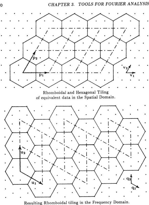
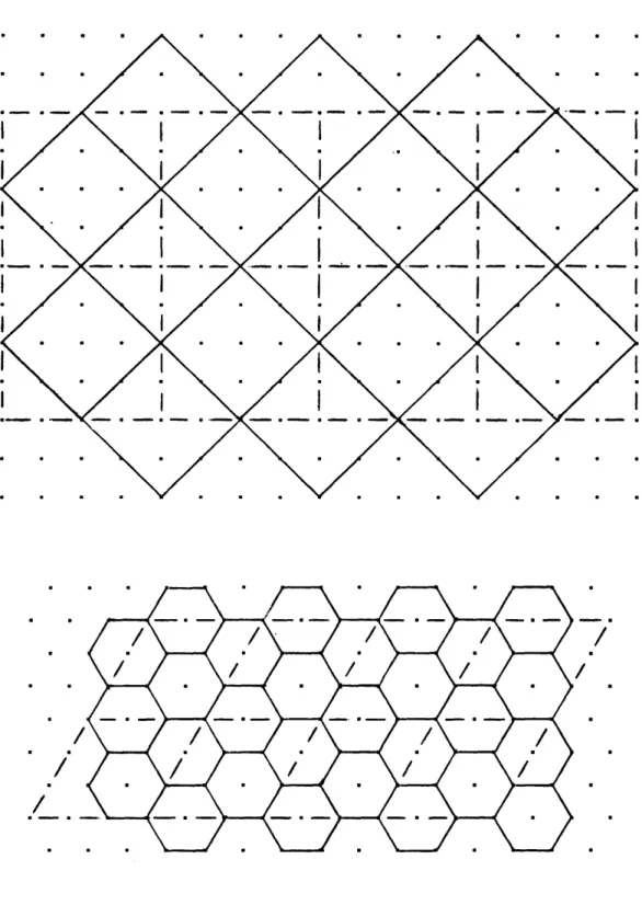
Rhomboidal Tiling of a Rectangular Array ...
Rhomboidal Tiling of a Hexagonal Array with an even period.. Packing odd periods into an even period ...
Segmentation Strategy for Spectral Estimation. ... 9 29 31 34 39 42 43 46 49 51 53 58 63 69 70 72 77 -._·L111 I--. . -l-LL-l---- -.---l.ll--PI
-·--Segmenting the Spectral Estimate into Concentric Annuli (2 pages) The dependence of 2 on gray level ...
Number of Frequency Samples within each Annulus ...
Rectangular Random Dither of a Gray Scale Ramp ... Rectangular Random Dither of a Scanned Picture ... Rectangular Random Dither of a Synthesized Image... Rectangular Radial Spectra for Random Dither (3 pages) .... Detail from a 1695 Mezzotint. ...
Hexagonal Random Dither of a Gray Scale Ramp ... Hexagonal Random Dither of a Scanned Picture. ... Hexagonal Radial Spectrum for Random Dither ...
5.1 Microphotographs of printed classical halftones (3 pages) 5.2 Orientation Perception of a 65 lpi screen.
5.3 5.4 5.5 5.6 5.7 5.8 5.9 5.10 5.11 5.12 5.13 5.14 ... .106
Spatial Frequency Sensitivity vs. Orientation ... Disparity in sensitivity to oblique and vertical gratings Threshold arrays for 45° Classical Screens (2 pages) 45° Classical Screen on a Gray Scale Ramp (3 pages) 450 Classical Screen on a Scanned Picture (3 pages) 450 Classical Screen on a Synthesized Image (2 pages) Composite Fourier Transform of the 45° Classical Screen Threshold array for a 0° Classical Screen ... 0° Classical Screen on a Gray Scale Ramp... 0° Classical Screen on a Scanned Picture ... Composite Fourier Transform of the 0° Classical Screen. Threshold arrays for Spiral and Line Screens. ... ... .107 ... .107 ... .109 ... .112 ... 115 ... .118 (3 pages) 120 ... 124 ... 125 ... 126 ... 127 ... 129 10 3.6 3.7 3.8 4.1 4.2 4.3 4.4 4.5 4.6 4.7 4.8 78 81 83 87 88 89 91 94 96 97 98 .... 103
5.20 Composite Fourier Transform of the Line Screen .... ... 135
5.21 Uncorrected Classical Screen on a Scanned Picture ... 137
5.22 Corrected Threshold Array for a grid with a = ... . 138
5.23 Corrected Classical Screen on a Gray Scale Ramp, a = . . 139
5.24 Corrected Classical Screen on a Scanned Picture, a = . 140 5.25 Composite Fourier Transforms with = . ... 141
5.26 Tri-state Ordering Scheme for the Hexagonal Classical Screen.. . 144
5.27 Threshold array for a 27 element Hexagonal Classical Screen. .. 144
5.28 Hexagonal Classical Screen on a Gray Scale Ramp ... 145
5.29 Hexagonal Classical Screen on a Scanned Picture... 146
5.30 Composite Fourier Transform of the Hexagonal Classical Screen. 147 5.31 Threshold array for a Hexagonal Spiral Screen ... 149
5.32 Hexagonal Spiral Screen on a Gray Scale Ramp. ... 150
5.33 Hexagonal Spiral Screen on a Scanned Picture. ... 151
5.34 Composite Fourier Transform of the Hexagonal Spiral Screen. .. 152
6.1 The first 8 Orders of Rectangular Tiles. ... 155
6.2 The first 5 Orders of Hexagonal Tiles. ... 156
6.3 Rectangular Recursive Tessellation ... 158
6.4 Hexagonal Recursive Tessellation (2 pages) ... 160
6.5 Rectangular Threshold Arrays (3 pages) ... 162
6.6 Hexagonal Threshold Arrays (2 pages) ... 165 11
6.7 Packing two odd ordered periods for rectangular storage .... 167
6.8 Packing two even ordered periods for rectangular storage .... 168
6.9 Rectangular Ordered Dither of a Gray Scale Ramp (8 pages) . 170 6.10 Hexagonal Ordered Dither of a Gray Scale Ramp (5 pages) . 178 6.11 Rectangular Ordered Dither of a Scanned Picture (5 pages) . . . 184
6.12 Rectangular Ordered Dither of a Synthesized Image (2 pages) . . 189
6.13 Hexagonal Ordered Dither of a Scanned Picture (4 pages) ... . 191
6.14 Importance of Hexagonal Kind ... 195
6.15 Detail from a 1844 silk weaving by the Jacquard loom ... 196
6.16 Rectangular Composite Fourier Transforms (8 pages) ... 198
6.17 Hexagonal Composite Fourier Transforms (5 pages) ... 206
6.18 Superposition of Square and Regular Hexagonal Basebands . . . 213
7.1 Failure of ordered dither on an asymmetric grid (2 pages) ... . 216
7.2 Sacrificing Resolution for Symmetry with ar=... .219
7.3 Complement Aspect Ratios Pairs ... 221
7.4 Ternary Subsampling of an Asymmetric Hexagonal Grid .... 223
7.5 Compensating Threshold Arrays by Ternary Replication .... 224
7.6 Hexagonal Subsampling of an Asymmetric Rectangular Grid. .. 227
7.7 Compensating Rectangular Arrays by Hexagonal Subsampling . 229 7.8 Compensated Threshold Array for < a, < 1. ... 230
7.9 Comparison of Gray Scale Ramp for a, = 2 (3 pages) ... 232
7.10 Comparison of Scanned Picture for a, (3 pages) ... 235
7.11 Comparison of Exposure Plots for a, = (2 pages) ... 238
7.12 Compensated Threshold Array for < < <. ... 241
7.13 Comparison of Gray Scale Ramp for ca, = 6 (4 pages) ... 242
7.14 Comparison of Scanned Picture for a, = G (4 pages) ... 247
Comparison of Scanned Picture for a, = (3 pages) ... 261
Comparison of Exposure Plots for a, =. .. 265
Principal Frequency, fg, as a function of g...
Patterns with the highest possible Spatial Frequency ... Spectral Characteristics of a Well Formed Dither Pattern. Point Processes. ...
The Error Diffusion Algorithm. ... Error Filters reported in the Literature. ...
Error Diffusion with the Floyd and Steinberg Filter (3 pages) Radial Spectra for the Floyd and Steinberg Filter (7 pages) . Error Diffusion with the Jarvis, et al. Filter (3 pages) ... Error Diffusion with the Stucki Filter (3 pages) ... Radial Spectra for the Jarvis, et al. Filter (7 pages) ... Two Processing Path Options ...
Failure of One Deterministic Weight Location ...
Effect of One Randomly Positioned Weight (2 page) ... Radial Spectra for One Randomly Positioned Weight (6 pages) Deterministic Part of a Two Weight Error Filter...
Effect of Two Deterministic Weights. ... Radial Spectra for Two Deterministic Weights ...
Effect of Two Weights on a Serpentine Raster (2 pages) ...
270 271 272 274 275 276 278 281 290 293 297 304 308 309 312 318 319 320 321 13 7.20 7.21 8.1 8.2 8.3 8.4 8.5 8.6 8.7 8.8 8.9 8.10 8.11 8.12 8.13 8.14 8.15 8.16 8.17 8.18 8.19 In-ant S --_.-L_~~ IIX---·---L1 - I---L--l_
__---14
8.20 Effect of Two 100% Random Weights (2 pages) ... 323 8.21 Effect of Two 50% Random Weights (2 pages) ... . 325 8.22 Radial Spectra for Two 50% Random Weights (5 pages) ... 327 8.23 Floyd and Steinberg Filter with a 30% Random Threshold (2 pages) 333 8.24 Floyd and Steinberg Filter with 50% Random Weights (3 pages) 335 8.25 Spectra for the F&S Filter with Random Weights (7 pages) . . . 338 8.26 Asymmetric Robustness of Error Diffusion (2 pages) ... 347 8.27 Error Diffusion with the Stevenson and Arce Filter (2 pages) . 350 8.28 Radial Spectra for the Stevenson and Arce Filter (7 pages) . . . 352 8.29 Two Hexagonal Error Filters to be Perturbed ... 359 8.30 Effect of Two 50% Random Weights on a Hexagonal Grid (2 pages)360 8.31 Effect of Four 50% Random Weights on a Hexagonal Grid (2 pages)362 8.32 Radial Spectra for the Stochastic Hexagonal Filter (7 pages) . . . 365
9.1 Digital "Laplacian" Filters, [nl . ... 376 9.2 Sharpening with a Rectangular Laplacian Filter. ... 377 9.3 Sharpening with a Hexagonal Laplacian Filter. ... 378 9.4 Comparison of Halftone Patterns for g = .Comparison~~~~~~ o. Haftn Pat .o . . . ...en .. 380
Along with text and graphics, images will become a generic data type in general purpose computer systems. This poses new problems for the system designer. To the user, displaying an image on any of a wide variety of devices must be as transparent as displaying ASCII documents. Office video displays with differing gray level capacity, laser printers, and home dot-matrix printers, all of various resolutions and aspect ratios must render a given image in a similar way.
A solution requires that associated with each device is a dedicated display preprocessor that transforms the digital image data to a form tailored to the characteristics peculiar to that device.
Digital halftoning, a key component of such a preprocessor, refers to any
algorithmic process which creates the illusion of continuous-tone images from the judicious arrangement of binary picture elements. It is often called spatial
dithering. This report addresses the problem of developing such algorithms that
best match the specific parameters of any target display device, modeled as the Physical Reconstruction Function.
Outside of using photographic film and some thermal sensitive materials, 15
_IILXIIWIYIII···ICI_·l Il*LII X -_--_ -.· __ _._·I ··-.I-Y1--··--·IIUIII-L·II)-LIII--Y----
-CHAPTER 1. INTRODUCTION
there does not exist a practical method of producing true continuous-tone hard copy. Computer hard copy devices are almost exclusively binary in nature. While the video displays associated with workstations and terminals are cer-tainly capable of true continuous-tone, they are often implemented with frame buffers that provide high spatial resolution rather that full gray scale capability. Such devices are designed for dot-matrix text and graphics; digital halftoning provides the mechanism to display images on them.
The literature is replete with approaches to this problem, but almost all of them implicitly assume target displays with nonoverlapping symmetrically spaced dots on a rectangular raster. Often the grids are not symmetric, es-pecially in the case of low resolution displays. It is frequently the case that resolution can be easily increased in one direction and not the other due to different physical constraints. Also, a conventional rectangular display can be made hexagonal by simply introducing a half pixel offset on every other line. Generalized techniques for halftoning on such grids are introduced in this report. Understanding the nature of the dither patterns created by various algo-rithms is enhanced by examining their representation in the frequency domain. New techniques for summarizing the frequency content of periodic and aperiodic patterns on both rectangular and hexagonal grids are also presented.
In describing the parameters of the Physical Reconstruction Function in the next chapter, a new aspect ratio immunity argument in favor of hexagonal grids is developed. While some halftoning schemes benefit from the use of hexagonal grids, it will be shown in Chapter 8 through revelations in the frequency domain, that a rectangular grid is preferred for others.
A list of the major symbols used throughout this report is organized in a Glossary starting on page 391. An explanation of the notational conventions 16
---CHAPTER 1. INTRODUCTION
1.1
Choice of Halftone Techniques
This is a study of controlled noise.
Contouring is a well known noise form resulting from coarse amplitude
quan-tizing; artificial contours or boundaries develop in slowly varying regions of pic-tures that are truncated to a limited number gray levels. An extreme example illustrated in Figure 1.1 is when the number of gray levels is limited to two. (A good rendition of the original images can be seen on pages 336 and 337.)
Here, the two test pictures that will be used throughout this text demon-strate dependence on image content. While the perception of gray level is com-pletely gone, much of the detail of the scanned image survives. But, because many of the details in the synthesized image fluctuate entirely above or below
the threshold, much of its content is obliterated.
Roberts [62] was the first to point out that dither does not increase noise energy, but simply redistributes that induced by fixed quantization in a way which makes it less visible. In the frequency domain, all of the error in coarse quantizing a fixed gray level is in the zero frequency (dc) term. A dithered rendition should have an error-free zero frequency term with all of the error scattered in higher frequency components.
Table 1.1 categorically lists the chapters which address particular halftone techniques. A gray level can be rendered by covering a small area with either a clustered or dispersed "dot". If a display device can successfully accommodate an isolated black or white pixel, then by far the preferred choice is dispersed-dot
·d I
Figure 1.1: Quantizing with a Fixed Threshold. (a) Scanned Picture. (See page 336.)
1111111_ ----11111
.-··II· -- ----·-C-rl·i .·itXrrlrrry·C*LI··-L----U---'lsl--L--
-20 CHAPTER 1. INTRODUCTION 0 -4 X M v cd xn Co. w ~C w bOXD E - 0-4 c e ww v " 0. b E " a 0 = -_= .I -
-Table 1.1: Categorization of Halftone Techniques.
halftoning which maximizes the use of resolution. A clustered-dot halftone mim-ics the photoengraving process used in printing, where tiny pixels collectively comprise dots of various sizes.
There is a choice of computationally complexity that can be accepted. A point operation in image processing refers to any algorithm which produces output for a given location based only on the single input pixel at that loca-tion, independent of its neighbors. For applications where the minimization of computation time and/or hardware is a premium, then a point operation is preferred. Of course, neighborhood operations generally produce higher quality results.
All of the methods listed in Table 1.1 are viable options with the exception of dithering with white noise, which is presented for heuristic reasons only. The concept of dithering with blue noise, introduced in Chapter 8, achieves the
uncorrelated features of white noise without the low frequency artifacts.
The preferred choice of a dispersed-dot point operation is ordered dither. The solution for hexagonal grids included in Chapter 6 proves to be the solution
4
white noise aperiodic point dispersed
5
ordered dither periodic point clustered
6, 7
ordered dither periodic point dispersed
8
blue noise aperiodic neighborhood dispersed
22 CHAPTER 1. INTRODUCTION
for asymmetric rectangular grids in Chapter 7.
All of these techniques can be used to augment a display with limited gray scale capability. To best examine the nature of patterns produced, the focus of this work will be on the worst case, that of binary displays. For devices that can display more that two levels of gray, a simple extrapolation is explained at the end of this report in section 9.3.
Several overviews of existing halftone algorithms have been written. Among them are surveys be Allebach [71, Jarvis, et al. [39], Stoffel and Moreland [81], and Stucki [82].
1.2
Image Rendering Systems
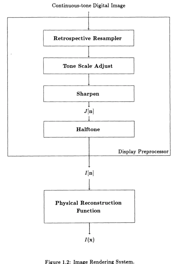
The display of high quality images on displays with only two levels of gray by halftoning can only be successful when performed as a component of the total image rendering system. The elements of such a system are identified in Figure 1.2.
The Physical Reconstruction Function is a system model of a given binary display device. It takes as its input a binary discrete-space image, I[n], and produces the continuous-space visual image, I(x). What happens in this step varies widely from device to device. It is here that the image data is given the physical dimensions of a grid geometry, with a "resolution" and aspect ratio. It is here that actual luminance values and dot structure are realized.
In a distributed system network, a given digital image may be displayed on any of several different hard copy and video devices. The role of the device dependent display preprocessor is to perform all the image processing manipula-tions necessary to transform a given continuous-tone digital image into a suitable intermediate binary digital image, I[n], that will yield the visible image when presented to the device.
The input to a halftoning process is a preprocessed continuous-tone digital image, J[n]. Halftoning is the last step in the display preprocessor seen in Fig-ure 1.2, after the other device dependent operations of Retrospective Resampler, Tone Scale Adjust, and optionally, Sharpen are executed.
The Retrospective Resampler is, in most cases, a digital scaler. Except for
I; _ ·_ilI___II _--·III^IYI--ICCI -C I ·I _ILIY1111·-l.·*liX-1IPIL·III-·Y--·
CHAPTER 1. INTRODUCTION
Continuous-tone Digital Image
I_ _ _ _ _ _____ Retrospectiv Tone Sca Sha J Hall re Resampler ile' Adjust rpen l [n] 1ftone ftone Display Preprocessor I[n]
I
Physical Reconstruction FunctionI
I(x)Figure 1.2: Image Rendering System. 24
l
.
one rectangular and the other hexagonal. The term retrospective resampling, adopted from an earlier work on scaling [851, describes the conceptual process of reconstructing the original continuous image from the given samples, then resampling this reconstruction.
A common method of performing such a reconstruction is through convo-lution with an appropriate interpolation function. Schreiber and Troxel have recently reported on the merits of such functions [73].
While resampling onto a new grid establishes the frame or "backbone" of the digital image, probably the most significant (and most underrated) contribution to image quality is tone scale. The simple point operation of mapping the gray level values of an image onto another distribution can have tremendous impact on the perceived quality of an image. The Tone Scale Adjust segment of the display preprocessor must compensate for the tone scale modification peculiar to the intended Physical Reconstruction Function in combination with the halftoning method to be used.
Once a halftoning algorithm has been selected for use on a particular de-vice, a gray scale ramp should be generated on that device for the purpose of calibration. Physical measurements of the reflectance (for hardcopy devices) or luminance (for luminous devices) should be made of the output gray scale to determine the compensating tone scale table to be employed in the display preprocessor.
The next element seen in Figure 1.2 is the Sharpen operation. Sharpening is optional but if it is to occur it should take place after resampling and before
CHAPTER 1. INTRODUCTION
halftoning. At this point, a distinction should be made between image enhance-ment and the integrity of an image rendering system. In most cases digital images "look better" if some sharpening is performed. Such an operation can be classified as image enhancement, a process that creates a changed image which, by some criteria, is better than the original. The technique of creating the illusion of a gray level by the judicious distribution of binary pixels, the essence of halftoning, tends to unsharpen an image; fine image detail can be lost in halftone patterns. Presharpening an image to compensate for this effect, to maintain as closely as possible the unadulterated integrity of the original image, is not enhancement in the usual sense.
In a well designed practical implementation, all of the operations in the display preprocessor should be carried out in one processing loop; there is no need to store intermediate images. However, these separate processes should not be compounded in the halftoning algorithm. They need to be controlled in a manner decoupled from one another.
The virtues of a halftoning method should be evaluated in terms of its ability to render the illusion of gray scale with minimum visibility of algorithmic arti-facts. Care must be used when evaluating methods which intrinsically sharpen. The "enhancement" perceived in the sharpened output can misleadingly out-weigh other shortcomings in the algorithms. The precise degree of sharpening should be controlled independently of halftoning.
.· I
1.3
Image Presentation Strategy
To assure a consistent and fair evaluation of all halftoning techniques to be presented, the same three specially selected source images are used throughout this text.
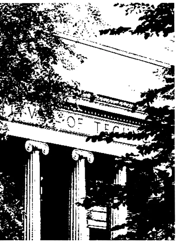
A historic picture of M.I.T. [55] of very high quality was digitized on both a rectangular and hexagonal grid with a constant number of samples per unit area. The image is a good test picture with textured and uniform regions, as well as areas of high detail such as the stone cut letters.
Scanned image data can sometimes benefit from noise inherent in the sam-pling process when halftoned. For that reason, a noiseless computer synthesized image borrowed from a work by Garcia [26] is occasionally shown for compari-son.
While a halftoning scheme may perform well rendering the gray levels seen in a particular picture, it may fail on others. For this reason, a wrapped tone scale ramp revealing all gray levels is always shown for both rectangular and hexagonal grids. The ramp proceeds linearly from white to black marked at the beginning with a one pixel wide black line for reference.
All digitally generated images were printed by an ECRM Autokon' 8400, a device whose design and operation is described by Schreiber [69,71]. The device is capable of very high resolution output, but by means of pixel replication, the images in this text are displayed at very low resolution (about 67 dots per
'Autokon is a trademark of ECRM.
CHAPTER 1. INTRODUCTION
inch for the case of a square grid). The reasons for this are to allow the reader to easily examine each of the dot patterns, and to assure that the images will survive reproduction. Higher resolution can be simulated by increasing the viewing distance. It should be noted that in the case of symmetric grids, the images in this text at the resolution shown would cover just over one square inch on a 300 dpi by 300 dpi display.
Several images are also shown on asymmetric rectangular grids, particularly in Chapter 7. To avoid overly small pixels for the same reasons stated above, the
smaller dimension of any rectangular pixel is fixed to that of the square grids, at
about 67 dots per inch. The other dimension will then have a lower resolution. Therefor, the overall resolution in pixels per unit area in this report is lower for images on asymmetric grids, by an amount proportional to the degree of asymmetry. For example, a picture shown on a grid with an aspect ratio of will have the number of pixels per unit area as that on a symmetric grid.
1.3.1
Tone Scale Adjustment
The process of printing and reproducing this report can itself be modeled with a Physical Reconstruction Function. One important characteristic that must be compensated for is the darkening due to broadening of black pixels which darkens images.
Figure 1.3 shows the actual tone scale adjustment curve used to prepare the rectangularly and hexagonally scanned images for the figures in this report. The transformation maps midrange gray levels to lighter values. (The straight superimposed line is a reference for a no-change transformation.)
Of particular importance are the horizontal portions at the top and bottom of the curve. They define the light and dark input ranges that are mapped to 28
0 1
Input Gray Level
Figure 1.3: Tone Scale Adjustment used for the Scanned Picture.
1 Q" so C5 aU -+,Go ;F? 0
30 CHAPTER 1. INTRODUCTION
complete white and complete black. Such a tone scale clipping creates an effect referred to as "snap" or "punch" in the graphic arts to pictures that would otherwise be described as "flat". The adjustment is especially important for
low resolution images as the ones in this report.
As an illustration of the dramatic difference a tone scale adjustment can make, Figure 1.4 is the scanned image used in all of the examples without the compensation of Figure 1.3. This should be compared to the identically halftoned picture on page 188.
Figure 1.4: "Scanned Picture" without Tone Scale Adjustment. Compare with Figure 6.11(e) (page 188).
CHAPTER 1. INTRODUCTION
Function
Understanding the nature of binary displays is central to designing high qual-ity halftoned images. The Physical Reconstruction Function, a general system model of a binary display shown in figure 2.1, is the topic of this chapter. The only feature of this model which makes the display binary is the fact that it will accept only binary input, that is, the input digital image, I[n], is a discrete set of ones and zeros.
The first section will address the details of the first block, D/C or the Discrete-to-Continuous Space Converter, which is a mathematically convenient mechanism to map a set of numbers to physical two-dimensional space. It is in that section that a new argument in favor of hexagonal grids is made in terms of aspect ratio.
In section 2.2 attention will be paid to the linear shift invariant function,
d(x), which governs the nature of an individual output dot along with the
generally nonlinear Tone Map, which assigns physical output luminances to 33
CHAPTER 2. PHYSICAL RECONSTRUCTION FUNCTION
I[n]
c(x)
I(x)
Figure 2.1: The Physical Reconstruction Function. 34
Noise
For completeness, two linear but space-varying components in the model of figure 2.1 are included to describe the stochastic characteristics of real physical devices.
Irregularities in the locations of dot centers is described by the Position Noise impulse. Dot-matrix impact printers have print wires that may wander in their solenoids. Perturbations in the dot positions of ink-jet printers are due to both aerodynamic and electrostatic interactions of drops in flight [44]. (x) would usually be a zero mean random process, or could have a nonzero mean at spatially dependent locations, such as seen in column misalignments.
Ink spread, dot size fluctuations, and other local degradations are described by the Dot Noise, w(x). The nature of this function can depend on anything from the size of the toner particles in laser printers [76] to the type of paper used [37].
Finally, to complete the Physical Reconstruction Function model, a "Back-ground", b(x), is added to describe the luminance from the paper or video phosphor used, along with any global degradations.
If the space varying, that is, the noise components are ignored, the relation-ship between the input and output of the Physical Reconstruction Function can be succinctly expressed as:
I(x) = TONE MAP (I[nl6(x - Vn)) * d(x) + b(x)
CHAPTER 2. PHYSICAL RECONSTRUCTION FUNCTION
the matrix, V, is described in the next section. 36
2.1
Grid Geometries
The content of this section is relevant not only to binary images and halftoning, but to digital image processing in general.
Perhaps the most important component of the Physical Reconstruction Function is the Discrete-to-Continuous Space Converter (D/C). It maps the input digital image, I[n], into a weighted set of delta functions in continuous space, c(x), expressed in vector notation as
c(x) = E I[n]6(x - Vn). (2.1)
n
It is in this step that the set of numbers, I[n], takes on real dimensions; the Discrete-to-Continuous Space Converter establishes resolution and aspect ratio. The nature of the impulses in equation (2.1) is the topic of this section.
2.1.1
Periodic Sampling Grids
A Periodic Sampling Grid is a two dimensional impulse train,
E 6(x - Vn), (2.2)
n
where the Sampling Matrix, V = [vl 1v
2], is composed of two linearly
indepen-dent Sampling Vectors,
VI i I V12 (2.3)
CHAPTER 2. PHYSICAL RECONSTRUCTION FUNCTION
with reference coordinate system, x, and index vector, n.
Figure 2.2 shows a periodic sampling grid in its most general form. The sampling vectors, vl and v2, can be thought of as grid generating vectors. Note
that if they were not linearly independent, the sampling grid would be only one dimensional.
Since antiquity, the format (frame shape) used for the overwhelming major-ity of painted and printed pictures produced has been rectangular, rather than rhomboidal as suggested by the sampling vectors or any other shape. So, the reference coordinate system (,x 2) should be orthogonal, as shown, regardless
of the grid pattern generated. The reference system can, without loss of gen-erality, be aligned anywhere. In this paper, the orthogonal coordinate system (x1',x2') is adopted.
Image data is almost always organized in lines for digitizing, storing, and displaying. It is convenient to refer to the coordinates, xl' and x2', as the
sample and line directions, respectively. Most often(but not always) the sample
axis refers to the horizontal direction, and the line axis refers to the vertical dimension. The sample period, S, is the distance between grid points in the sample direction, and the line period, L, is the distance between lines. In terms of the sampling vectors, S = Ivl and L = Iv21 cos 6, where 0 is the angle between vl and v2.
Figure 2.2 also illustrates a natural way of defining pixel shape. Pixel Shape is defined as the smallest circumscribing polygon about a given grid point con-structed from the perpendicular bisectors of lines between that point and all other grid points. Actual dot functions are most often circular in shape. The size of the circles is chosen to be just big enough to achieve complete coverage of the plane. For dots of this size and shape, an equivalent definition of pixel
l
Figure 2.2: General Periodic Sampling Grid with associated Pixel Shape.
-__ _L 11_1__ _ 1___11·___- X--
CHAPTER 2. PHYSICAL RECONSTRUCTION FUNCTION
shape results: The polygon surrounding a grid point whose vertices are the intersections of circles of this size centered at each grid point. Note that for periodic sampling grids, pixels will always be either "hexagonal parallelograms" or rectangles. It should be noted that the area of such pixels is always S x L regardless of its shape.
2.1.2
Semi-Regular Grids
A general periodic sampling grid, that is, one with v2 uncontrained, has two
shortcomings. Firstly, there is a lack of symmetry in the pixel shape and in the neighborhood surrounding it. Secondly, the offset for every line on an orthogonal coordinate system is different. This fact adds considerable complexity to simple image operations like cropping and scaling, or to the design of displays.
Semi-regular Grids are defined as Periodic sampling grids whose
correspond-ing pixel shapes are symmetric about at least two axes. There are two classes of semi-regular grids:
1. Rectangular Grids, where vl v2 = 0, (that is, vl I v2).
2. Semi-regular Hexagonal Grids, where vl .2 = v112/2,
(or IV21 COS = Iv1/2).
Note that semi-regular hexagonal grids require only one offset of exactly S/2 for every other line on an orthogonal coordinate system. Such grids have been referred to as "offset sampled" or "quincuncial". The familiar case of rectangular grids requires no offset.
An appropriate name for the shape of a pixel on semi-regular hexagonal grids is semi-regular hexagon. Of course, the shape of pixels on rectangular grids is rectangular. A useful metric which completely describes the shape of pixels on
2.1.2.1 Effect of Aspect Ratio
Aspect ratio is a parameter that often varies among display devices, particularly binary devices, but is seldom addressed theoretically. The effect of aspect ratio on pixel shape is shown for rectangular grid in figure 2.3 and for semi-regular hexagonal grids in figure 2.4.
The shape of the pixel on a rectangular grid is a regular polygon, a square, for only one value of a (a 1). The shape of pixels on semi-regular hexagonal grids is much more interesting. There are two cases where the pixel is a regular hexagon, for a = 2 and a = 23, and one special case where it is square, a = 2.
To avoid confusion between the two kinds of hexagons, a Hexagonal Grid of
the First Kind is defined to be a semi-regular hexagonal grid with a < 2 (see
the top row of figure 2.4). A Hexagonal Grid of the Second Kind is defined to be a semi-regular hexagonal grid with a > 2. (see the bottom row of figure 2.4). Mersereau [53,54] has shown that for a circularly band-limited waveform, sampling with a regular hexagonal grid involves 13.4% fewer samples to avoid aliasing (spectral overlap) than sampling with a square grid. This packing effi-ciency argument has long been recognized as one of the most important features of regular hexagonal grids. More recently, it has been shown [52] that hexagonal sampling produces samples with greater intersample dependency which allows "lost" samples to be more accurately recovered or restored. Another important argument can be made for semi-regular hexagons.
In practical display devices, the physical constraints governing the size of
PHYSICAL RECONSTRUCTION FUNCTION
a -. 5
aI-I
a -2
Figure 2.3: Pixel Shape on Rectangular Grids as a function of Aspect Ratio, a.
_ _
o
a= .7 C = 2
C73 5 a = 1.6
a = 23 a = 5.7
Figure 2.4: Pixel Shape on Hexagonal Grids as a function of Aspect Ratio, a.
a = 2.5 - - . - - - -_ -_ ~ ~ ~ * -_.ll_.lll·LI 1II__1II 1^1
CHAPTER 2. PHYSICAL RECONSTRUCTION FUNCTION
the sample and line periods, S and L, are often very different. Accepting these values as fixed, a given rectangular pixel device can be converted into a hexag-onal device by means of a very simple modification, introducing an alternate line offset of S/2. Assuming that the actual dots produced by the device are circles with a radius just large enough to achieve complete coverage of the image plane, a reasonable measure of performance is to compare the covering efficiency of the two arrangements. Note that in each case, rectangular and semi-regular hexagonal, the aspect ratio and number of pixels per unit area remain constant.
Covering Efficiency as a function of aspect ratio is defined as
Pixel Area
Circumscribing Circle Area
A high covering efficiency is a desirable property for several reasons. Higher
E(a) means
1. less dot overlap and thus a more linear tone scale rendition,
2. more similarly sized isolated black and white pixels, and
3. less spectral overlap (aliasing) for circularly band limited images.
As stated earlier, it can easily be shown that in all cases, pixel area is S x L. The radius, r, of the circumscribing circle is equal to the distance from the pixel center to any of its vertices. Simple geometry reveals that
2+ L2 for rectangular grids.
r =+ S for hexagonal grids, a < 2.
8L 4L2
+ 2 for hexagonal grids, a > 2.
4S
E(a) = 64a
- 1'
r(4a-1 + ay)2 for hexagonal grids, a < 2. (2.4)
16 for hexagonal grids, > 2.
~r(4a+ for hexagonal grids, a> 2. ·4a- 1 + a):
This function, plotted in figure 2.5, reveals several interesting features. On a plot as this one where the abscissa, x, is equal to the logarithm of a, a is proportional to eZ and the rectangular function of equation (2.4) takes the form of a hyperbolic secant, as evidenced by its shape in figure 2.5. The hexagonal curve is bimodal, peaking at E = ~ z .827 at the two aspect ratios where the pixel shapes are regular hexagons. At the cusp (a = 2), where the hexagonal grid has square pixels, the covering efficiency, E = .637, is precisely that of the peak of the rectangular grid at a = 1.
Probably the most important observation is that while semi-regular hexago-nal grids outperform rectangular grids at all aspect ratios, they achieve covering efficiencies better than or equal to the best rectangular case for aspect ratios be-tween .591 and 6.77!
Digital halftoning employs binary displays where, particularly in the case of lower resolution devices, each pixel adds an appreciable contribution to the quality of the output. Along with the increased symmetry and decreased aliasing arguments, the relative "immunity" of hexagonal grids to aspect ratio make it an important alternative to rectangular grids.
__YI1 II^II_-_·L- ~ I 1I-
CHAPTER 2. PHYSICAL RECONSTRUCTION F UNCTION 2 22v'i 2 r 2 VI
ilI
Aspect Ratio, a
Figure 2.5: Covering Efficiency of Pixels on Semi-regular Grids as a function of Aspect Ratio.
46
I. A
Ja)
a) Q eE b n n1(
'Table 2.1: Some Major Display Classes
2.2
Dot Function and Tone Map
The dot function, d(x), is the linear space invariant component of the display with superposition described by convolution, while the generally nonlinear Tone Map assigns physical output luminances to input values. Next to the Discrete-to-Continuous Space Converter, it is these two components that most distinguish display devices.
Table 2.1 identifies some basic classes of binary displays. The five classes shown are not expected to be exhaustive, but exemplify target models for halftone display.
Electroluminescent Plasma Panel
II Pillbox Hard Step Wire Impact (carbon ribbon) III Pillbox Soft Step Ink-jet
Wire Impact
IV Gaussian Hard Step Electrophotographic (Laser) Offset Printing
CHAPTER 2. PHYSICAL RECONSTRUCTION FUNCTION
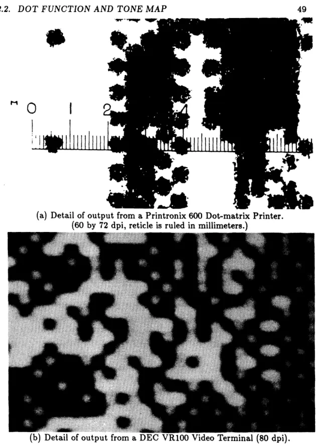
Most existing halftoning algorithms are implicitly designed for Class I dis-plays (with square grids). This, the simplest class, includes any display with nonoverlapping dots. The resulting luminance depends only on the number of dots turned on, independent of any Tone Map. The other classes in table 2.1 all have overlapping dot functions. The Tone Maps for these classes are all de-scribed as "steps" since they eventually clip the output at some minimum and maximum. "Hard" steps have no transition region between the two extremes, and thus do not increase density at areas of overlap. Photographic close-ups of a Class II device (a), and Class V devices (b and c) are shown in figure 2.6.
A very important type of binary display is Class IV, which includes the pop-ular laser printers. Plain paper laser printers operate by charging or discharging a photosensitive drum with a scanning laser illumination, leaving a latent image to which oppositely charged toner particles are attracted. Existing products are described as "positive" or "negative" printers depending on whether the laser erases white or writes black.
An example of how the dot function, d(x), can itself be composed of several linear components cascaded together in convolution is shown qualitatively in figure 2.7 for class IV and V devices. Sonnenberg [78,79] of Xerox has carefully studied the tradeoffs that must be considered in setting the parameters for d(x) in laser printers. To maintain the integrity of primitives occurring most often in text, thin horizontal and vertical lines are usually favored at the expense of isolated pixels, and thus dispersed-dot halftoning on such devices yield very nonlinear results.
Figure 2.8 illustrates both the nonlinearities and diversity in laser printer output. Since this is a cursory rather than thorough comparison of two products, the names "Product X" and "Product Y" is used to protect the innocent. The 48
I
I
1111111
(a) Detail of output from a Printronix 600 Dot-matrix Printer. (60 by 72 dpi, reticle is ruled in millimeters.)
Figure 2.6: Photographic Enlargements of Binary Display Output.
--Y --l---1L--- --- ---II--· - I l l ,
50 CHAPTER 2. PHYSICAL RECONSTRUC.
Figure 2.6 (continued)
(c) Detail of output from an ECRM Autok4 (740 dpi, reticle is ruled in millimeters.)
TION FUNCTION
:On.
Beam Shape
One Period Pulse
Video Bandwidth
2
X1
Figure 2.7: Cascaded Components of a "Gaussian" Dot Function.
J;1
31
,,1
52 CHAPTER 2. PHYSICAL RECONSTRUCTION FUNCTION
difference between figure 2.8 (b) and (c) is due to a tighter dot size and smaller toner particles in (c); both printers are "positive" in that the laser erases white area.
Figure 2.8: Diversity and Nonlinearity in Laser Printer Output. (a) Exact data to be printed, simulated by the Autokon.
54 CHAPTER 2. PHYSICAL RECONSTRUCTION FUNCTION
Figure 2.8: Diversity and Nonlinearity in Laser Printer Output (continued). (b) Detail of output from "Product X".
(300 dpi, reticle is ruled in millimeters.)
_ ____________________·
i9-. 4"-~j
. o , s.-
: W.
Figure 2.8: Diversity and Nonlinearity in Laser Printer Output (continued). (c) Detail of output from "Product Y".
CHAPTER 2. PHYSICAL RECONSTRUCTION FUNCTION
2.3
Reflectance and Luminance
It is customary to assign zero to the amplitude of a digital image sample if no output is to be produced at that location. This leads to two conventions; the hardcopy convention assigns zero to the unmarked white paper, while the convention for luminous displays, such as CRTs, assigns zero to the dark screen. In this report, the hardcopy convention is adopted, and the gray level, g, is proportional to reflectance. Reflectance is defined as the ratio of reflected to incident radiant power. g = 0 corresponds to the reflectance of the unmarked white paper, Rw, and g = 1 to the reflectance, RB, generated by all black output pixels. The desired macroscopic output reflectance is then
R = Rw + (RB - Rw) (2.5)
For the case of perfectly diffuse reflection copy, the luminance, , observed at any angle and given illumination is directly proportional to the reflectance.
£ = £w + g(£B + w) (2.6)
= LB + (1 - g)(£w + £B) (2.7)
For the luminous display convention, equation (2.7) would best describe the relationship between the desired output luminance, , and the "gray level" amplitude, (1 - g).
In either case, if dots do not overlap, then a halftoning scheme should create the desired output by setting the ratio of black dots to total dots in a given region of uniform gray level to g. However, dots usually do overlap.
that is, displays with perfect circular dots where density does not increase at areas of dot overlap.
Allebach [6] describes a solution for an imaginary device that has overlapping pixels that are perfectly square and have sizes that are exact integer multiples of the grid period. Roetling [67] examined one particular plotter with a fixed dot size. He proposed computing the overlap into a cell due to all combinations of its eight nearest neighbors, then using that information to create a compensated classical halftone screen. Similar geometric solutions were proposed to compen-sate for dot overlap in the error diffusion algorithm, a dispersed-dot technique for rectangular [831 and hexagonal [80] grids.
2.3.1 Direct Measurement
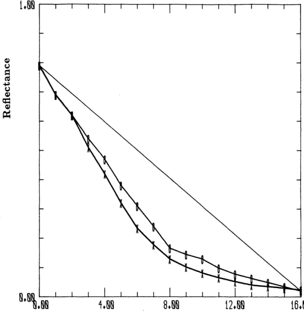
It appears the the most reliable means of compensating for nonlinearity in tone scale (reflectance or luminance) is to use the information from direct measure-ment of output from a candidate device with a given halftone technique. The suitability of a clustered of dispersed-dot method can be established, and a compensating tone scale transformation can then be made prior to halftoning.
The reflectance of three hard copy devices was measured and plotted in figure 2.9, as a function of covering 4 x 4 periods with increasing number of black output pixels with the dispersed-dot patterns of figure 6.9(d) (page 173). In each of the three plots, Rw and RB are slightly different, due to the differences in whiteness of the papers used, and blackness of the maximum densities which can be achieved.
PHYSICAL RECONSTRUCTION FUNCTION
Black Units per 4 x 4 block
(a) Xerox 2700 laser printer.
(Exhibits failure to accommodate dispersed-dot patterns.)
1.8
8.8%s
Black Units per 4 x 4 block
(b) Printronix 600 dot-matrix printer. Figure 2.9: Example Reflectance Measurements.
.l.,S
IX* BSS
4.
9
12.SS
16.M
Black Units per 4 x 4 block
Figure 2.9: Example Reflectance Measurements (continued). (c) ECRM Autokon.
"X" for individual dots, "0" for groups of 3 x 3 dots.
Q Q 0 0) 1 +D U w V V M n - 0It 1_-1--_11_-- ·I-- ··--_IIUI-·I-C---·i·---·
--11--^-CHAPTER 2. PHYSICAL RECONSTRUCTION FUNCTION
Figure 2.9(a) illustrates the failure of a particular laser printer to accom-modate dispersed-dot halftoning. The inability of this device to reliably print isolated black pixels results in a tone scale which is not only nonlinear but nonmonotonic. Clustered-dot halftoning is necessary for this device.
The devices measured in (b) and (c) of figure 2.9 can support dispersed-dot halftoning, but are nonlinear. Accounting for dot overlap and even the increase in density at regions of overlap is only part of the reason for this nonlinearity.
To minimize the effect of dot overlap, the 720 dpi Autokon generated the same patterns with "super pixels" composed of 3 x 3 Autokon dots. The output was effectively from a 240 dpi device with nearly square dots. The measured reflectance curve for this case is shown on the same plot as the measurements for patterns generated with individual dots in figure 2.9(c). The disparity from linearity in reflectance was reduced but not nearly to the degree that would be predicted by the reduction in dot overlap.
If the surface onto which a halftone was printed was completely opaque, then the reflectance could indeed be exactly calculated based on the percentage of area covered. Surprisingly, multiple internal reflections within paper contributes appreciably to the nonlinearity of reflectance, a phenomenon recognized over 30 years ago [16j. This effect depends on the translucency and thickness of the paper, as well as the size and distribution of dots on the top surface.
Considering the complexity and number of parameters that contribute to the relationship between gray level, g, and output reflectance, R, the best method of calibrating tone scale is direct measurement.
The Fourier Transform has been employed in the past to evaluate halftoned images, but only very special cases of even period ordered dither on square grids were considered [3,41,63] In this chapter, comprehensive methods for analyzing the nature of all types of patterns produced by halftoning will be developed in the frequency domain for both rectangular and hexagonal grids.
The most characteristic feature of a halftone technique is the texture gener-ated in areas of uniform gray. The rendition of high frequency detail depends primarily on how sharp the image was (or to what extent high pass filtering was performed) prior to halftoning. As stated earlier, some degree of presharpening will usually produce higher quality halftoned pictures.
The best measure of the virtues of a halftone algorithm, then, is its ability to render areas of uniform gray. The approach used to examine this ability in the frequency domain depends on whether or not the resulting binary texture patterns are periodic. This chapter is divided into two part to address each case separately. Introduced are "exposure plots" of Composite Fourier Transforms which will present insight into the nature of the periodic output of ordered
61
--- __.___._ _ ___,_II_-X ll__l___ ___
-CHAPTER 3. TOOLS FOR FOURIER ANALYSIS
dither, and Radially Averaged Power Spectra along with a measure of anisotropy to provide a mechanism for studying aperiodic patterns.
3.1
Periodic (Ordered) Patterns
The ordered dither algorithms of Chapters 5, 6, and 7 halftone by thresholding or "screening" with periodic threshold arrays. The binary output from such halftone processes will also be periodic with the same spatial period as the threshold array. The spatial period will be specified by two vectors, pi and P2, in terms of the spatial sampling vectors, vl and v2, described in section 2.1.1.
The spatial periods can be thought of as tiles which cover all of two-space. Two types of periods are of interest. Figure 3.1 shows examples of odd and even
periods' (tiles) on semi-regular rectangular and hexagonal grids of the first kind.
Since rectangular tiles share each vertex with 4 other tiles, and each edge with 2 other tiles, only 1 vertex and 2 edges are unique to each tile. By a similar argument, only 2 vertices and 3 edges are unique to each hexagonal tile. The outlined edge and vertices in figure 3.1 show those points which are not part of the unique period.
Even periods are replicated by period vectors that are collinear with the sampling vectors,
pi=Nv, (3.1)
P2=NV2, for some integer, N. Odd periods are defined by
p,=N(v, + v2)
(3.2)
P2=N(v2 - v2).
'Describing periods as "odd" or "even" is consistent with period order, r1, introduced in
Chapter 6.
I
Odd Even Figure 3.1: Odd and Even Spatial Periods
for rectangular grids (top) and hexagonal grids of the first kind (bottom). Boundary locations which are not part of the unique period are outlined.
* · · · * · · I a a * a * I -·--- --- ---·---·- ·--- - -I · · · · · · · · · · · · · · · · · · · · · · · · · · · · · · ·
CHAPTER 3. TOOLS FOR FOURIER ANALYSIS
It is important to note that two odd periods on a rectangular grid and three odd periods on a hexagonal grid can always be packed into one even period.
The derivation of a general expression for the Fourier Transform of periodic patterns with an even period is addressed in the following section.
3.1.1
Continuous-space Fourier Transform Computation
For nonrectangular grids, it is not immediately clear how a discrete Fourier Transform can be computed, or what its dimensions in continuous frequency space are. So, a method of computation along with an explicit expression in continuous space is sought.
Probably the first formalization of the Fourier representation of nonrectan-gularly sampled spaces was by Petersen and Middleton in 1962 [60]. Mersereau later specifically addressed hexagonally sampled signals with his derivation of the Hexagonal Discrete Fourier Transform (HDFT) [54). But this expression is complicated, primarily because hexagonal periods can not in general be rear-ranged to repeat in a rectangular (rhomboidal) fashion.
For the case where the number of elements in a hexagonal period, or any shaped period, on a general periodic sampling grid is a perfect square, the following is a proof inspired by the multidimensional sampling theorem [19] that the canonical rectangular DFT can be used to compute its Fourier Transform.
Proof
The two-dimensional continuous space Fourier Transform, C(fl, f2), of an im-age, c(xl,:x2), can be expressed as
C(fl, f2) = Y{C(XI, X2)}
J /
C(X1, X2)e-j2r(flzl+f2z2)dxldX2C(f)= fc(x)} = c(x)e-2fTxdx (3.3) _00
c(X) = f-{C(f)} = f C(f)eJ2rfTXdf (3.4)
-00
The units of the frequency components in these expressions are cycles/unit-length as opposed to the more common radians/unit-cycles/unit-length.
One important identity that will be used is the transform of a two-dimensional impulse train:
{6(x-An ) I detAl m ( (3.)
where BTA = I,
detA = aja 2 2 - a2a2l,
and represents E E.
n nl=-oo n2=-00oo
Note that the spatial pixel area as defined in section 2.1.1 is equal to I det Al,
the frequency "pixel area" is det B , and I det Al = det BI - . The matrix B
can be expressed explicitly as
)T a22 -a2l
B = (A-')T = (3.6)
detA -a 1 2 all
Recalling that V has been defined as the spatial sampling matrix (equations (2.2) and (2.3), page 37),
. 6(x - Vn) I det VI (f U ) (3.7)
n Jdet~ m
TOOLS FOR FOURIER ANALYSIS
Suppose c(x) is a periodic array of weighted impulses on the sampling grid of equation (2.2) with an N x N rhomboidal shaped period. It could be expressed
as c(x) = (I[nl 6(x - n)) 0* * 6(x-Pl) I (3.8)
where "*" denotes two-dimensional convolution,
N
n
represents
N N
n l -=-0 n2=0
I[n) is a discrete-space image, and P = [pi P2 = NV is the spatial period
replication matrix. Note that 6(x - P1l) 1 00 - d e PI
Z
E c(f - Qk) kwhere Q = [ql ' q2] = (p-)T is the frequency sampling matrix. Q also equals
-U, since P = NV and U = (V-1)T.
The Fourier Transform of this image is
C(f) = {c(x)} e j2,rfTxdx) (na I[n]e -i2~rfTVn) n 1 X 1 >det 6(f - Qk) det P k 1 °° ldet l 6(f - Qk).
This expression is zero everywhere except at f = Qk, so the frequency term in the exponent becomes
fT = kTQT
where QT = V since Q = (p-1)T and P = NV.
Thus, equation (3.10) becomes simply
I(n]e- kTn) 6(f - Qk) (3.9) (3.10) 66 CHAPTER 3. 5r
E00
I
1: I[njb(x - Vn) nCC(f)
=
~tE 1:
(3.11)N N
I[k = I[k1,k2l = E E I[ni,n2 leN(k +k2n2) (3.12)
n I =O n2=O
is recognized as the familiar two-dimensional discrete Fourier Transform! Equation (3.11) satisfies the need for an explicit expression in continuous frequency space and a simple mechanism for computation.
Check of Proof
For completeness and as a check for this proof, the reverse Fourier Transform can be computed in a similar way. Since I[k] is also periodic with period N x N,
1 N 0o
C(f) d= dt I[kl6(f - Qk)) * >Z(f - Um) (3.13)
and its inverse Fourier transform is
c(x) = -1{C(f)}
= det PI - Qk) e 2'rfdf) detVIZ6(x -Vn)
d E (6t I[kle 2 )7 (x - Vn) (3.14)
} detPI k
where QT 1 V 1 again simplifies the exponent.
The expression is further simplified by observing that I det PI = N 2 det Vl,
so
0oN 0 o
c(x) = E I[n]6(x - Vn) = E I[n16(x - Vn) * E 6(x - P1) (3.15)
n n 1