Differentiable Volume Rendering using Signed
Distance Functions
by
Srinivas Kaza
B.S., Massachusetts Institute of Technology (2019)
Submitted to the Department of Electrical Engineering and Computer
Science
in partial fulfillment of the requirements for the degree of
Masters of Engineering in Electrical Engineering and Computer Science
at the
MASSACHUSETTS INSTITUTE OF TECHNOLOGY
September 2019
c
○Srinivas Kaza, 2019. All rights reserved.
The author hereby grants to M.I.T. permission to reproduce and to
distribute publicly paper and electronic copies of this thesis document
in whole and in part in any medium now known or hereafter created
Author . . . .
Department of Electrical Engineering and Computer Science
August 23, 2019
Certified by . . . .
Fredo Durand
Professor
Thesis Supervisor
Accepted by . . . .
Katrina LaCurts
Chair, Masters of Engineering Thesis Committee
Differentiable Volume Rendering using Signed Distance
Functions
by
Srinivas Kaza
Submitted to the Department of Electrical Engineering and Computer Science on August 23, 2019, in partial fulfillment of the
requirements for the degree of
Masters of Engineering in Electrical Engineering and Computer Science
Abstract
Gradient-based methods are often used in a computer graphics and computer vision context to solve inverse rendering problems. These methods can be used to infer camera parameters, material properties, and even object pose and geometry from 2D images.
One of the challenges that faces differentiable rendering systems is handling visi-bility terms in the rendering equation, which are not continuous on object boundaries. We present a renderer that solves this problem by introducing a form of visibility that is not discontinuous, and thus can be differentiated. This “soft visibility” is inspired by volumetric rendering, and is facilitated by our decision to represent geometry within the scene as a signed distance function. We also present methods for performing gra-dient descent upon distance fields while preserving Lipschitz continuity. Unlike most differentiable mesh-based renderers, our renderer can optimize between geometry of different homeomorphism classes in a variety of image-based shape fitting tasks. Thesis Supervisor: Fredo Durand
Acknowledgments
I would like to thank my advisor Fredo Durand, for encouraging and mentoring my UROP in computer graphics while I was a sophomore, for motivating my SuperUROP as a junior, and finally for guiding me with this thesis as a senior. Fredo’s compu-tational photography class was one of my favorite courses at MIT; it was a fun and rewarding experience that showed me how to combine two of my hobbies – computer programming and photography. For introducing me to computer graphics (and com-putational photography) research, and continuing to mentor me along the way, I am truly grateful.
I would also like to thank Lukas Murmann. Fredo introduced me to Lukas during my sophomore year, and he has been an amazing source of help, advice, and mo-tivation during my UROPs and SuperUROP, as well as this Masters thesis. Lukas has always been a source of thoughtful commentary and support, regardless of the project.
He also introduced me to Tzu-Mao Li, who had already established the technical foundations for my masters thesis through his wonderful work on the Halide au-tomatic differentiation framework, differentiable ray tracing through edge sampling (and redner), and differentiable volumetric rendering. I deeply appreciate his ex-pertise in differentiable rendering, as well as his willingness to help debug the myriad of issues that arose when I tried to write a differentiable volume renderer in Halide.
I would like to thank the friends and peers who have helped make MIT feel like home. Finally, I would like to thank my parents, and my sister. Their support and encouragement have been invaluable from my first day at MIT until the last.
Contents
1 Introduction 11
1.1 Motivation . . . 12
1.2 Overview . . . 12
1.3 Outline and Contributions . . . 13
1.3.1 Contributions . . . 15
2 Background 17 2.1 Automatic Differentiation . . . 17
2.1.1 Forward-mode and Reverse-mode Differentiation . . . 18
2.2 Signed Distance Fields . . . 20
2.3 Differentiable Rendering . . . 21
2.4 Halide . . . 22
3 Volume Rendering 25 3.1 Forward Pass . . . 25
3.2 Backwards Pass . . . 28
4 Distance Field Optimization 33 4.1 Lipschitz Continuity . . . 33
4.2 Distance Preserving Gradient Update . . . 34
4.3 Convex Quadratic Programming . . . 35
4.4 Fast Marching Method . . . 35
5 Implementation 41
5.1 Backwards Pass Implementation . . . 42
5.1.1 Checkpointing . . . 43
6 Results and Discussion 45 6.1 Experiments . . . 45
6.1.1 Rigid Transform . . . 45
6.1.2 Multi-View Reconstruction . . . 47
6.2 Discussion . . . 48
List of Figures
1-1 Overview of Optimization Process . . . 14
2-1 Expression Graph Example . . . 19
2-2 Derivative Graph Example . . . 20
3-1 The Effect of Varying the 𝜎 Parameter . . . 28
3-2 Trilinear Interpolation of Normals . . . 31
4-1 Quadratic Programming Gradient Update . . . 36
4-2 Fast Marching Method Gradient Update . . . 38
6-1 Inferring a Rigid Transform from a Single Image . . . 46
6-2 Rigid Transform Fitting Loss . . . 46
6-3 Target Views of Bunny . . . 48
6-4 Optimizing a Sphere into a Bunny . . . 49
6-5 Bunny SDF Visualization . . . 50
6-6 Bunny Optimization Loss . . . 50
Chapter 1
Introduction
Computer vision systems endeavor to understand or reconstruct the parameters of a scene from one or more images. On the other hand, computer graphics systems endeavor to depict or render images given a description of a scene. Thus, it is un-surprising that there is a persistent view of computer vision as inverse computer graphics [20]. In its simplest form, one can describe the process of rendering as the function 𝑓 (𝜃), and as such, the goal of inverse rendering is merely to minimize the error 𝐸(𝜃) = ‖𝑓 (𝜃) − 𝐼‖, where I is the ground truth image.
This simple explanation of the inverse problem belies the practical challenges of designing an inverse renderer. The large space of renderable images, as well as the complexity of the forward rendering pipeline, means that the optimization strategy will be specialized for the task of rendering. Differentiable rendering is a process which describes the output of the rendering process (i.e individual pixels) as a func-tion of scene parameters, and provides the derivative as a funcfunc-tion of those same parameters. Combined with a suitable gradient-descent optimization method, one can use a differentiable renderer to approach the inverse rendering problem.
This thesis describes the background, design decisions, and implementation details of our differentiable renderer. We also present a couple inverse rendering experiments performed using our renderer and their results.
1.1
Motivation
Volumetric reconstruction, illumination estimation, pose estimation, and material identification are all important computer vision problems that can be used to gen-erate content for 3D applications. Most photo-realistic 3D content, however, is not created from real world data because existing computer vision approaches tend to solve only one or two of these problems at a time. In the context of machine learning, novel view synthesis approaches [17] [16] [38] [15] have become popular options for specialized reconstruction problems, like 3D face reconstruction. These methods typ-ically use deep learning approaches to create new viewpoints from a small number of observed viewpoints. Unfortunately, these methods do not have any understanding of light transport, and they often struggle to generalize beyond their training sets in a physically-consistent manner.
Differentiable renderering might be an answer to this problem. A differentiable renderer, such as the one outlined in this thesis, is a way of describing the physics of light transport in a manner that can be optimized using gradient descent. While we chose to evaluate our differentiable renderer as a standalone tool for 3D reconstruction tasks, we believe that differentiable renderers can be used as building blocks for more complex computer vision applications. For example, our differentiable renderer could be used to construct adversarial examples for neural networks [3] [21].
1.2
Overview
Any general-purpose differentiable rendering system must properly account for the discontinuous nature of visibility. The visibility terms present in the volumetric ren-dering integral are not differentiable across the silhouette of an object or across occlu-sions. Because the visibility terms in the rendering integral effectively resemble the step function on object boundaries, sampling the gradient at these locations is equiv-alent to sampling the Dirac delta function. As a result, the gradient is not properly dispersed across the volume.
Our method uses signed distance functions to represent geometry. A signed dis-tance function of a set Ω in a metric space determines the disdis-tance of a point 𝑝 from the object boundary of Ω, and is positive when 𝑝 is outside the object boundaries and negative otherwise.
Signed distance functions have been used for a variety of purposes in both com-puter graphics and comcom-puter vision literature. For example, they are used in image segmentation tasks, where segmentable objects are represented via different signed distance functions [6]. Within computer graphics, signed distance functions have been used to render anti-aliased fonts and implicit surfaces.
In particular, our renderer renders the implicit surface of signed distance field using volumetric ray marching. Signed distance fields are generally not used for volume rendering, as they describe a surface rather than a volume with participating media. However, our volumetric representation of a signed distance field closely describes the implicit surface while remaining differentiable on object boundaries. Several methods are presented to ensure that the distance field remains renderable over iterations of gradient descent.
Our results demonstrate that this renderer is capable of performing a variety of inverse rendering tasks, including inferring rigid-body transforms from a single view and 3D multi-view reconstruction. Unlike most approaches which render meshes, our signed distance field renderer can optimize for complex geometry that is not homeomorphic to the initialization. Modifying the connectivity of a mesh during optimization is a difficult problem, which is why most mesh-based differentiable ren-derers assume that the initialization mesh has similar connectivity to the target image [21] [23]. Our approach is completely unsupervised and does not involve any deep learning components, unlike many modern differentiable renderers [24] [23] [18].
1.3
Outline and Contributions
Chapter two describes the background behind this project, including previous work in differentiable rendering and other inverse rendering endeavors.
initialize SDF render SDF (forward pass)
compute gradient (backward pass) perform gradient update using ADAM correct distance field to
be Lipschitz continuous target image SDF target image render, SDF gradient, SDF updated SDF renderable SDF
Figure 1-1: Overview of Optimization Process. Our differentiable rendering pipeline is similar to most other renderers, except that the gradient descent process can make the geometry invalid. Thus, a correction step in which the geometry is made Lipschitz continuous is necessary.
Chapter three describes the volumetric rendering integral, and how it shapes our form of soft visibility. This section also includes an explanation of derivative of the volumetric rendering approach and some commentary about efficient implementation strategies.
Chapter four describes several approaches to optimizing the distance field based on the computed gradients. A brief discussion of the validity of a distance field is included here.
Chapter five describes the implementation of the differentiable rendering system in Halide and CUDA.
Chapter six details the efficacy of using the proposed differentiable ray tracer, and what these results mean.
1.3.1
Contributions
∙ We specify and implement a differentiable volume renderer of signed distance fields.
∙ We detail several methods to maintain the validity of the distance field during gradient updates.
∙ We perform several small experiments to evaluate the effectiveness of our method and interpret the results.
Chapter 2
Background
This chapter outlines prior work in automatic differentiation, implicit surface mod-eling, and other differentiable rendering approaches. A quick overview of the Halide language is also included in this chapter.
2.1
Automatic Differentiation
Gradient descent optimization requires computing the gradient of the model function with respect to the parameters. The final goal is to minimize a cost function – which is typically the mean squared error between the output generated from the inferred parameters and the target. The purpose of optimization is to infer the parameters of the model which produce a result which is similar to the target.
To perform gradient descent optimization upon a function, the gradient of that function must be computed. Some functions include loops, control flow, or recursion. Some functions are discontinuous. Automatic differentiation frameworks differentiate these programs by splitting composite functions into their components, and taking the derivative of each independently.
Automatic differentiation computes the derivative of each individual operation and then joins the results together using the chain rule. The framework only needs to have knowledge of the symbolic derivative of each operation, such as the the deriva-tive of the exponential function. Intermediate results are stored and factored out of
other expressions which refer to them. On the other hand, symbolic differentiation utilities, often included in mathematical toolkits like Sage [36] or Mathematica [14], usually do not perform this kind of reasoning and will inline intermediate results. The symbolically-derived derivatives can be challenging to generate (especially with a sufficiently complex function or many symbols), and are usually less efficient than their automatic counterparts because intermediate expressions are not stored.
An alternative to both automatic differentiation and symbolic differentiation is to simply approximate the derivative using finite differences. This approach is inaccurate and scales with the dimension of the input vector. However, finite differences are a useful tool for debugging the results of automatic differentiation as well a means of approximating derivatives of non-parametric functions. Our renderer uses a finite difference to approximate the spatial gradient of the signed distance field to obtain surface normals (see equation 3.8).
2.1.1
Forward-mode and Reverse-mode Differentiation
Forward-mode and reverse-mode differentiation are two ways in which the derivatives of an expression graph can be computed. Forward-mode differentiation computes the derivatives of each node in the graph, starting from the inputs and moving forward through the computational graph to the outputs. The primary issue with forward-mode differentiation is that the derivative for each output value must be computed with respect to every single input variable. Our input vector is the signed distance field itself, which can easily comprise thousands of voxels. However, any given ray may only reference a small number of these voxels. Thus, it makes little sense to use forward-mode differentiation for these cases.
Reverse-mode differentiation works by computing the derivative with respect to the outputs and then working backwards through the graph to the inputs. When computing derivatives of 𝑓′(𝑥) using reverse-mode differentiation, the intermediate functions of 𝑓 (𝑥) are needed. Thus, to compute 𝑓′(𝑥), we must first compute 𝑓 (𝑥). The initial step of computing 𝑓 (𝑥) is referred to as the forward pass, and the process of computing 𝑓′(𝑥) is called the backward pass.
+
+
A *
B C
Figure 2-1: Represents A + (B * C) + (B * C)
Machine learning frameworks usually include a mechanism for performing auto-matic differentiation. The inclusion of autoauto-matic differentiation on arbitrary expres-sion graphs makes sense given the use of backpropagation for neural networks [32]. The PyTorch machine learning framework [28] automatically creates an expression graph and computes derivatives using reverse-mode differentiation.
As an example, Figure 2-1 is an expression graph which represents the expression,
𝐴(𝑥) + (𝐵(𝑥) * 𝐶(𝑥)) + (𝐵(𝑥) * 𝐶(𝑥)) (2.1)
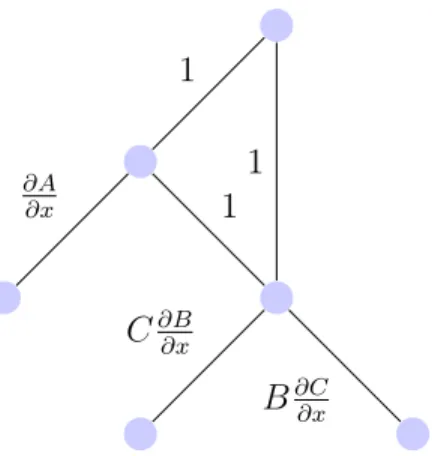
In an expression graph, the vertices are values and the edges are operations that use those values. The derivative of any expression graph can be expressed in a deriva-tive graph, where the edges represent the derivaderiva-tive of the parent vertex with respect to the child vertex. Figure 2-2 represents the corresponding derivative graph (with respect to 𝑥).
The derivative is simply the sum of the product of the elements on each path. Forward-mode and reverse-mode differentiation can be expressed as different methods of traversing the paths of this graph.
The D* algorithm efficiently performs reverse-mode differentiation by factoring out subgraphs of the derivative graph [11]. The optimizations performed by D* are similar to the tail recursion optimization performed in section 5.1. The Opt
1 1 𝜕𝐴 𝜕𝑥 1 𝐶𝜕𝐵𝜕𝑥 𝐵𝜕𝐶 𝜕𝑥
Figure 2-2: Represents the derivative of A + (B * C) + (B * C)
programming language allows a programmer to express a non-linear least squares optimization problem and automatically generate a solver for it. The D* algorithm is used to create the derivative graph for the solver.
2.2
Signed Distance Fields
Beyond their role in implicit surface rendering [13] and font rendering [9] in the field of computer graphics, Signed distance fields have found use in many 3D reconstruction applications. For example, the Kinect Fusion system approaches the 3D reconstruc-tion problem by computing a truncated signed distance funcreconstruc-tion using point cloud data from an RGBD sensor [27]. The truncated signed distance field clamps the distance from [−1, 1] to simplify integration.
As stated in the previous section, a signed distance function returns the distance to the implicit surface of the object, positive if the evaluation position is outside the volume and negative if it is inside the volume. One can render the implicit surface of the signed distance function through sphere tracing [13], or by extracting a mesh using the marching cubes algorithm [26].
Learning-based approaches have also used signed distance functions to represent geometry [7] [37]. Many of these approaches involve generating a 3D volume which represents the signed distance field. The convolutional layers often used in deep learning architectures to isolate 2D features in images can be adapted to 3D volumes.
Polygon meshes are often unsuitable for these applications because modifying the connectivity of the mesh during geometry optimization is difficult. We decided to use signed distance fields for the same reason.
2.3
Differentiable Rendering
Most inverse-rendering and differentiable rendering work tries to limit the scope of the problem. Blanz and Vetter [5] focused on synthesizing textured 3D faces. Barron and Malik [4] infer shape, illumination, and simple material properties from single images. More recently, OpenDR [25] and the Neural 3D Mesh renderer [18] have attempted to provide a more general-purpose differentiable rendering framework by rasterizing the scene and then using a finite difference approximation upon the color buffer (see section 2.1) to estimate the derivative. Both of these methods assume Lambertian materials and do not handle indirect illumination and shadowing.
Many of these differentiable rendering systems fail to properly account for the non-differentiable nature of visibility. Because the visibility terms in the rendering integral are not differentiable on object boundaries, many of the solutions mentioned above will often fail to propagate gradients when either the object or the camera changes position. Our approach solves this problem by introducing “soft visibility” – the concept that object boundaries have soft falloffs rather than hard boundaries (see section 3.1 for an overview of the approach).
Li et al. [21] used a novel edge sampling method to properly handle the non-differentiable rendering terms in the rendering equation. Note that the edges of objects appear as step functions in the visibility terms – the gradient of these step functions is the Dirac delta function which cannot be sampled directly. In continuous regions (i.e those within object boundaries), the standard approach with automatic differentiation is sufficient. However, in discontinuous regions (i.e triangle edges), both the foreground and the background of the edge are sampled, and contributions from both sides are correctly handled. Overall, this approach is easily extensible to secondary visibility effects, and was implemented as a fully differentiable Monte Carlo
path tracer.
Rhodin et al. [31] presented an early differentiable volumetric ray caster which can perform marker-less object pose estimation as well as marker-less full-body motion capture. Their approach bears certain resemblances to ours – in particular, they also use a Gaussian density distribution to model soft visibility. Our approach focuses on optimizing the geometry of signed distance fields for inverse rendering applications rather than optimizing parametric models that represent skeletons, although one of our experiments learns a rigid body transform.
Liu et al. [23] introduced a differentiable rendering approach which aggregates contributions from all mesh elements and then fuses them together according to the probability that a given triangle will contribute to a screen-space pixel. Like the work by Rhodin et al. [31], this formulation of soft visibility has similarities to ours. However, like the previously-mentioned differentiable rendering frameworks, this method does not attempt to compute secondary visibility effects. The use of polygon meshes to represent geometry means that this technique may have difficulty optimizing for geometry that is not homeomorphic to the initialization.
Most recently, Lombardi et al. [24] developed a differentiable volume ray marcher to facilitate rendering complex and translucent surfaces like skin and hair. An encoder-decoder network transformed 2D images into their 3D volumetric represen-tation. A warp field, learned in tandem with the rest of the volume parameters, is used to improve the spatial resolution. Their method learns a color and opacity buffer, and the quality of the reconstructed volumes is comparable with commercial photogrammetry software like Agisoft Metashape [2]. Our approach learns geometry represented by signed distance fields rather than color and opacity volumes. Addi-tionally, our renderer does not currently include any deep learning component.
2.4
Halide
The Halide language emerged to facilitate the development and optimization of multi-stage image processing pipelines [30]. Optimizing image processing code is a
chal-lenging process which typically involves experimenting with many different orderings of the intermediate functions, which are then composited to produce the final output of the pipeline. The optimal ordering depends on the availability of specific hard-ware features, or the amount of resources provided (cache size, amount of available memory, number of cores, SIMD architecture, etc.,). When optimization encourages obfuscation, readability is often a secondary priority. Portability is another issue with the traditional image processing pipelines. For example, Grand Central Dispatch on OS X serves the same role as thread pools and task queues on other operation sys-tems. CUDA, OpenCL, Metal, Vulkan, DirectX, and OpenGL provide interfaces for general purpose GPU programming at varying degrees of abstraction. Each combi-nation of platforms could require a dedicated code path, and heterogeneous compute only complicates the problem.
Halide attempts to solve this problem by introducing a distinction between algo-rithms and schedules. In Halide, an algorithm is a composition of functions which describe an image processing pipeline. The schedule describes when these functions should be computed, if they should be stored, and where to store them. Once the correctness of the algorithm has been determined, the programmer can be confident that modifying the schedule will not introduce regressions.
One implementation of the volumetric renderer was written in Halide. The gradi-ents were computed using the Halide automatic differentiation framework [22]. The Halide automatic differentiation framework is carefully designed to properly handle “gather” operations, like convolutions (the output dimension is small and the input dimension is large). The derivative of a gather operation is a “scatter” operation (the output dimension is large and the input dimension is small). Scatter operations can be performed using global atomic operations, although these operations can be slow if there is high contention. Our CUDA implementation uses a scatter operation across the signed distance field to accumulate the gradient (see section 5.1 for details). The Halide automatic differentiation framework describes scatter operations as another gather operation before storing the output [22], which is often more efficient than using atomics.
Chapter 3
Volume Rendering
This chapter presents the volume rendering approach employed by the the differen-tiable ray tracer described in this thesis. Many other differendifferen-tiable rendering ap-proaches do not have robust means of differentiating the discontinuous integrand (see section 2.3 for an explanation of the problem). The rendering model outlined in the following section attempts to address this issue.
3.1
Forward Pass
Our approach uses a volume scattering model to create a “soft” falloff at object bound-aries. As a result, the derivative of the rendering integrand can be properly sampled. The model relies on a spatially-varying attenuation coefficient 𝜑𝑡(𝑡) = 𝜑𝑡(𝑝 + 𝑡𝜔),
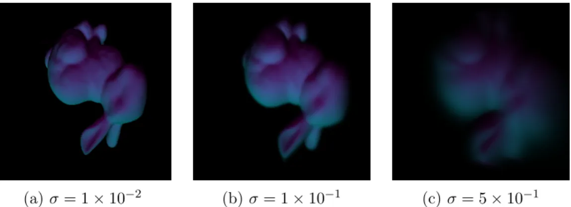
which represents out-scattering and absorption over the ray. The chosen attenuation function is Gaussian, and the standard deviation of that function (see 3.9 and Figure 3-1) determines the density of the medium.
𝐿𝑖(𝑝, 𝜔) =
∫︁ 𝑡𝑚𝑎𝑥
0
𝑇𝑟(𝑝 + 𝑡𝜔 → 𝑝)𝐿𝑠(𝑝 + 𝑡𝜔, −𝜔) (3.1)
Equation 3.1 represents the integral form of the equation of transfer [29], ignor-ing the surface interaction. 𝑇𝑟 is the beam transmittance. The light source term
𝐿𝑠(𝑝, 𝜔) = 𝜑𝑠(𝑝)
∫︁
𝑆2
𝑝(𝑝, 𝜔′, 𝜔)𝐿𝑖(𝑝, 𝜔′)𝑑𝜔′ (3.2)
𝑝(𝜔, 𝜔′) is the phase function, representing the angular distribution of scattered radiation. As mentioned earlier, the medium is heterogeneous, and is sampled using ray-marching [29]. The sampling PDF can be expressed as
𝑝𝑡(𝑡) = 𝜑𝑡(𝑡)𝑒− ∫︀𝑡
0𝜑𝑡(𝑡 ′)𝑑𝑡′
(3.3) Our implementation adds an additional intensity term 𝐼(𝑝, 𝐷), which represents the BSDF evaluated at the isosurface represented by the signed distance function 𝐷 at 𝑝. 𝐿𝑖(𝑝, 𝐷, 𝜔) = ∫︁ 𝑡𝑚𝑎𝑥 0 𝜑𝑠(𝑝, 𝐷(𝑝𝑡))𝐼(𝑝𝑡, 𝐷)𝑒− ∫︀𝑡 0𝜑𝑡(𝑡 ′,𝐷(𝑡′))𝑑𝑡′ 𝑑𝑡 (3.4)
Ray-marching involves discretizing the range [0, 𝑡𝑚𝑎𝑥] into a series of small
seg-ments and approximating the integral in each region. In practice, this implies that we can rewrite this integral as an iterative process with an update rule. We refer to 𝑂𝑡 as the approximated integral of 𝜑𝑡 from [0, 𝑡], and ℎ as the step size.
𝑂𝑡+1(𝑝𝑡+1, 𝐷) = 𝑂𝑡(𝑝𝑡, 𝐷(𝑝𝑡)) + 𝜑𝑡(𝑝𝑡, 𝐷(𝑝𝑡))ℎ (3.5)
𝐿𝑡+1(𝑝, 𝐷, 𝜔) = 𝐿𝑡+ 𝜑𝑠(𝑝, 𝐷(𝑝𝑡))𝐼(𝑝, 𝐷)𝑒−𝑂
𝑡+1
ℎ (3.6)
It is not difficult to implement these equations in a space and time efficient man-ner. Both the Halide and the CUDA implementations perform reductions over the 𝑡 domain. Most of the implementation challenges arise when computing the derivatives. 𝐷(𝑝) represents the trilinear interpolation of the signed distance function 𝐷 at location 𝑝. The signed distance function is represented by an array of voxels, and the 𝐷(𝑝) interpolates between these voxels. Given an 𝛼 vector that describes the fractional offset from 𝑝0 and 𝑐𝑖𝑗𝑘 representing the vertices of the unit cube between
𝛼 = 𝑝 − 𝑝0 𝑝1− 𝑝0 𝑐00= 𝑐000(1 − 𝛼𝑥) + 𝑐100𝛼𝑥 𝑐01= 𝑐001(1 − 𝛼𝑥) + 𝑐101𝛼𝑥 𝑐10= 𝑐010(1 − 𝛼𝑥) + 𝑐110𝛼𝑥 𝑐11= 𝑐011(1 − 𝛼𝑥) + 𝑐111𝛼𝑥 𝑐0 = 𝑐00(1 − 𝛼𝑦) + 𝑐10𝛼𝑦 𝑐1 = 𝑐01(1 − 𝛼𝑦) + 𝑐11𝛼𝑦 𝑐 = 𝑐0(1 − 𝛼𝑧) + 𝑐1𝛼𝑧 (3.7)
The intensity function 𝐼(𝑝, 𝐷) relies on the surface normal at the isosurface as part of the BSDF. The surface normal is computed by performing the 3D Sobel filter across the SDF [12]. The Sobel filter is a simple first-order derivative operator that is composed of a differentiation and averaging kernel. The direction of the spatial gradient can be used to approximate the normal (i.e the output of the Sobel filter is normalized). The intensity function samples the surface normal using trilinear interpolation of the resulting voxel array.
ℎ(−1) = 1, ℎ(0) = 2, ℎ(1) = 1 ℎ′(−1) = 1, ℎ′(0) = 0, ℎ′(1) = −1 𝑠𝑥 = ℎ′(𝑥)ℎ(𝑦)ℎ(𝑧) 𝑠𝑦 = ℎ′(𝑦)ℎ(𝑧)ℎ(𝑥) 𝑠𝑧 = ℎ′(𝑧)ℎ(𝑥)ℎ(𝑦) (3.8)
𝜑𝑠(𝐷(𝑝)) and 𝜑𝑡(𝐷(𝑝)) are based on the Gaussian PDF. As a result, the
atten-uation coefficient is greater in regions that are closest to the level set of the SDF and lesser in regions that are far away from the surface. To properly render closed surfaces, the distance to the surface is clamped at zero as an input into 𝜑.
𝜑(𝑥, 𝜎) = √ 1 2𝜋𝜎2𝑒
−max(0,𝑥)2
(a) 𝜎 = 1 × 10⁻² (b) 𝜎 = 1 × 10⁻¹ (c) 𝜎 = 5 × 10⁻¹
Figure 3-1: The Effect of Varying the 𝜎 Parameter. Increasing 𝜎 increases the radius of the attenuation function 𝜑, blurring the final image. 𝜎 controls the spread of gradient contributions across the signed distance function; large values of 𝜎 will allow optimization to converge quickly while smaller values will converge slowly or not at all.
Finally, an adaptive step size was considered to expedite iterations of ray marching. The ray marching step size at 𝑝 would vary linearly with the value of 𝐷(𝑝). This approach works well, and an adaptive step size can reduce the number of iterations of ray marching by a factor of three or more. We decided to use a fixed step size because the dependency between 𝑝 and 𝐷(𝑝) complicates the backwards pass.
3.2
Backwards Pass
Derivatives for equation 3.6 are computed using reverse-mode differentiation. Reverse-mode differentiation starts from the outputs of the computational graph and propa-gates derivatives backwards, eventually reaching the inputs. This method of differ-entiation works well when there are many inputs and few outputs (see section 2.1.1 for an overview of the differences between forward and reverse-mode differentiation). Our initial Halide implementation used the Halide automatic differentiation sys-tem [22] to compute the derivatives in this section. For the CUDA implementation, the backwards pass was written by hand.
While the gradients of nearly all of the parameters (e.g camera orientation/pa-rameters, material properties, object pose, etc.,) of the differentiable renderer can be computed, this chapter will focus on the derivatives of the signed distance function
itself. The derivatives of the intensity function will also be omitted, as they vary depending on the BSDF used. Joint optimization of multiple scene parameters is also possible, although doing so was not a focus on this thesis.
When computing derivatives using reverse-mode differentiation, one often needs to compute the forward pass as well. Thus, there exists a memory-space trade-off between caching intermediate results of the forward pass and recomputing them from scratch (see section 2.1 for background on this topic). This chapter will ignore the details of “checkpointing” results from the forward pass for now. For implementation details, see section 5.1.1.
The process concludes with the derivative of the incoming light (equation 3.6) with respect to all of the parameters in the signed distance function.
𝜕𝐿𝑡+1 𝜕𝐷𝑖𝑗𝑘 = 𝜕𝐿 𝑡 𝜕𝐷𝑖𝑗𝑘 + 𝜕(𝜑𝑠(𝑝 𝑡, 𝐷(𝑝𝑡))𝐼(𝑝𝑡, 𝐷)𝑒−𝑂𝑡+1 ℎ) 𝜕𝐷𝑖𝑗𝑘 (3.10) As mentioned in section 3.1, 𝑡 represents iterations of ray marching. The back-wards pass begins with the last iteration of ray marching and works backback-wards to compute the gradient with respect to the signed distance function. 3.10 can be ex-panded as follows: 𝜕𝐿𝑡+1 𝜕𝐷𝑖𝑗𝑘 = 𝜕𝐿 𝑡 𝜕𝐷𝑖𝑗𝑘 + ℎ𝐼(𝑝𝑡, 𝐷)𝜑𝑠(𝑝𝑡, 𝐷(𝑝𝑡))𝑒−𝑂 𝑡+1𝜕𝑂𝑡+1 𝐷𝑖𝑗𝑘 + ℎ𝐼(𝑝𝑡, 𝐷)𝑒−𝑂𝑡+1𝜕𝜑(𝑝 𝑡) 𝜕𝐷𝑖𝑗𝑘 + ℎ𝜑(𝑝𝑡)𝑒−𝑂𝑡+1𝜕𝐼(𝑝 𝑡, 𝐷) 𝜕𝐷𝑖𝑗𝑘 (3.11)
Recall that 𝐷𝑖𝑗𝑘 represents the entirety of the signed distance function, and 𝜕𝐷𝜕𝐿
𝑖𝑗𝑘
is the gradient across the entirety of the signed distance function. However, at each iteration of equation 3.11, gradients are greater than zero at only a few locations in the signed distance function. These locations are referenced by either the trilin-ear interpolation of the signed distance function or the trilintrilin-ear interpolation of the normals. Thus, the gradient is accumulated as a sum across every ray evaluation po-sition. The practical implication of this observation is that the memory consumption
of this algorithm is most affected by the trilinear interpolation of the normals. See section 5.1 for details.
Ideally, equation 3.11 could be rewritten using tail recursion and performed iter-atively. Doing so greatly reduces the amount of memory required for reverse-mode differentiation, as the stack frame would contain information about all prior ray eval-uations on the current ray. Care must be taken to ensure that recursive calls to 𝑂 (equation 3.5) are properly inlined into 𝐿. 𝜕𝑂𝜕𝐷𝑡+1
𝑖𝑗𝑘 is substituted into 𝐿 𝑡+1 to obtain 𝜕𝐿𝑡+1 𝜕𝐷𝑖𝑗𝑘 = 𝜕𝐿 𝑡 𝜕𝐷𝑖𝑗𝑘 + ℎ𝐼(𝑝𝑡, 𝐷)𝜑𝑠(𝑝𝑡, 𝐷(𝑝𝑡))𝑒−𝑂 𝑡+1 (𝜕𝜎𝑡(𝑝 𝑡, 𝐷(𝑝𝑡)) 𝐷𝑖𝑗𝑘 + 𝜕𝑂 𝑡 𝐷𝑖𝑗𝑘 ) + ℎ𝐼(𝑝𝑡, 𝐷)𝑒−𝑂𝑡+1𝜕𝜑(𝑝 𝑡) 𝜕𝐷𝑖𝑗𝑘 + ℎ𝜑(𝑝𝑡)𝑒−𝑂𝑡+1𝜕𝐼(𝑝 𝑡, 𝐷) 𝜕𝐷𝑖𝑗𝑘 (3.12)
Recursively computing 𝑂, storing the results, and then computing 𝐿 would be prohibitively expensive. Thus, the approach is to rewrite 3.12 as
𝜕𝐿𝑡+1 𝜕𝐷𝑖𝑗𝑘 + 𝑐𝑡+1𝜕𝑂 𝑡+1 𝜕𝐷𝑖𝑗𝑘 = ... (3.13)
On the iteration 𝑡 (i.e the first iteration of the backwards pass), 𝑐𝑡+1 is 0, making this equation the same as 3.12. After evaluating the terms in 3.12, the term associated with 𝑂𝑡 is added to 𝑐𝑡+1 to obtain 𝑐𝑡. Storing 𝑐𝑡 between iterations is not difficult because it is a scalar.
Each ray evaluation accumulates a contribution to the gradient at every location in the SDF accessed at that iteration. Most of the terms in 3.12 include the deriva-tive of the trilinear interpolation of the signed distance function (𝜕𝐷(𝑝𝜕𝐷 𝑡)
𝑖𝑗𝑘 ). Trilinear
interpolation accesses the eight neighboring voxels of a floating-point position in the coordinate system of the voxel grid. Thus, these terms reference the eight neighbor-ing voxels of the ray evaluation position. However, the intensity term references the surface normal. This surface normal is computed by trilinearly interpolating between values in the normals voxel array. The Sobel filter references the 27 spatial neighbors
of a given voxel (i.e the 3x3x3 neighborhood around the voxel). Given that the surface normal is the result of trilinearly interpolating the voxel array of normals, a 4x4x4 neighborhood of the gradient is computed.
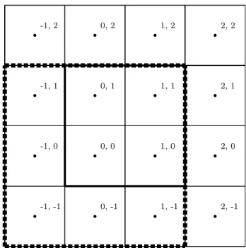
-1, -1 -1, 0 -1, 1 -1, 2 0, -1 0, 0 0, 1 0, 2 1, -1 1, 0 1, 1 1, 2 2, -1 2, 0 2, 1 2, 2
Figure 3-2: Voxels affected by trilinear interpolation of normals. Because the intensity function references the trilinear interpolation of the normals at a point between (0, 0, 0) and (1, 1, 1), all 8 normals voxels between and including (0, 0, 0) and (1, 1, 1) receive gradients. Each one of these voxels was computed from all of its 27 neighbors (represented by the dotted line). A total of 64 voxels of the signed distance function receive gradients from this operation.
Chapter 4
Distance Field Optimization
This chapter discusses methods for performing gradient descent upon the signed dis-tance field. Naively performing a gradient descent algorithm like stochastic gradient descent or ADAM [19] will not necessarily produce a renderable distance field. Thus, a new optimization strategy is needed to perform the gradient descent update while also preserving the continuity of the distance field.
4.1
Lipschitz Continuity
A function R3 → R is Lipschitz continuous under the 𝐿
2 norm if, for some
non-negative constant 𝐶 ∈ R, so that
𝑝1, 𝑝2 ∈ R3 : |𝑑(𝑝1) − 𝑑(𝑝2)| ≤ 𝐶|𝑝1− 𝑝2| (4.1)
where 𝑝1, 𝑝2 are points within the domain of the distance field. The signed distance
function must be Lipschitz continuous for 𝐶 = 1.
Equivalently, the magnitude of the derivative of the signed distance function is bounded by 𝐶.
4.2
Distance Preserving Gradient Update
A naive approach to optimization would involve performing the forward pass, com-puting gradients during the backwards pass, and then performing gradient descent upon the values of the signed distance field using these gradients. However, most gradient descent algorithms, like ADAM or stochastic gradient descent are not viable options because the update procedure will violate Lipschitz continuity.
Additionally, while Lipschitz-continuous distance fields are renderable, they may provide an underestimate of the true distance function. The correct approach to solving this problem is to solve the Eikonal equation 4.2, rather than just satisfying Lipschitz continuity.
|∇𝑖𝑗𝑘𝑑(𝑝)| = 1 (4.2)
Consider the gradient update (R3 → R)∇𝑑(𝑝)
𝑑𝑡+1= 𝑑𝑡(𝑝) − 𝜂∇𝑑(𝑝) (4.3)
As stated earlier, this is not a distance preserving operation. We want to find the correction 𝑥 which will minimize
𝑑𝑡+1𝑐𝑜𝑟𝑟𝑒𝑐𝑡𝑒𝑑 = 𝑑𝑡+1(𝑝) + 𝑥𝑡+1(𝑝) (4.4)
where 𝑑𝑐𝑜𝑟𝑟𝑒𝑐𝑡𝑒𝑑 is a valid distance field (i.e one that satisfies the Eikonal equation).
We have implemented several optimization techniques that satisfy these require-ments. The simplest approach is to re-distance the signed distance function from the level set using the Fast Marching Method. We also considered using quadratic programming to update the distance field according to the gradient vector while also enforcing the Eikonal equation constraints. Finally, the quadratic programming approach inspired a simpler soft constraint which was represented as an additional penalty in the cost function.
4.3
Convex Quadratic Programming
Quadratic programming solves problems of the following form:
Minimize 1
2𝑥
𝑇𝑄𝑥 + 𝑐𝑇𝑥
subject to 𝐸𝑥 = 𝑑
(4.5)
If 𝑄 is positive definite, then the problem is convex.
Written as a quadratic programming problem, the goal is to minimize the correc-tion vector 𝑥 – i.e constrained least squares. 𝑄 is just the identity matrix, which is symmetric and positive definite.
Lipschitz continuity can be imposed by limiting the magnitude of the gradient in all dimensions.
|𝜕𝑑 𝜕𝑑𝑖
| < 1 (4.6)
The gradient is approximated by an eighth-order central difference. The distance field is convolved accordingly and represents the Lipschitz constraint in E.
The Eikonal equation cannot be expressed as a linear constraint. A quadratic con-straint is needed, which would be difficult to solve efficiently. A limited workaround which produces acceptable results is to constrain the solutions to the Eikonal equation with linear bounds. For example, the Eikonal equation is lower-bounded by the L1 norm of the gradient, and upper-bounded by the tangent hyperplane at the angle 𝑝𝑖4. More linear constraints can be added in a similar fashion, creating a tighter bound, but these constraints seem sufficient so far.
4.4
Fast Marching Method
While the quadratic programming approach mentioned in the previous section works well, it is too computationally expensive to be used after every iteration of train-ing. The fast marching method [33] was considered to simply regenerate the signed distance function from the zero crossings after each gradient update.
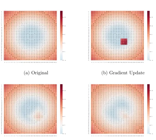
(a) Original (b) Gradient Update
(c) Optimization w/o L1 constraint (d) Optimization w/ L1 constraint
Figure 4-1: Quadratic Programming Gradient Update. The signed distance function in 4-1a represents a circle, and 4-1b represents a gradient update to the signed distance field. 4-1c is the result of performing the quadratic programming approach with only Lipschitz continuity constraints. The lower-right region is underestimated. 4-1d incorporates the L1 constraint and the corresponding tangent line constraint, mitigating this issue.
The fast marching method solves boundary value problems that are of the form
|∇𝜑(𝑥)| = 1
𝑓 (𝑥) ∀𝑥 ∈ Ω
𝜑(𝑥) = 0 ∀𝑥 ∈ 𝜕Ω
(4.7)
where 𝜑 represents the time required for the point 𝑥 to be on the surface of the signed distance function. The algorithm for performing iterations of the fast march-ing method has a strong resemblance to Dijkstra’s algorithm.
Data: 𝑈 (𝑥𝑖) = 𝜑(𝑥𝑖)
Result: computes 𝑈 (𝑥𝑖)∀𝑖
Set all 𝑈 (𝑥𝑖) to ∞, except for the nodes in the zero crossing which should be
0
Label the nodes in the zero crossing as accepted while there exists 𝑥𝑖 not in accepted do
For every node that isn’t already accepted, update 𝑈 (𝑥𝑖) by finding the
neighbor with the distance value of the smallest magnitude and adding the distance to the neighbor to that value;
Add the 𝑈 (𝑥𝑖) with the distance of the smallest magnitude to accepted;
end
Algorithm 1: An overview of the fast marching method
The fast marching method can re-initialize the signed distance field given an ex-isting set of zero-crossing values (i.e the uncorrected surface). Our approach simply examines the neighbors of a voxel to determine whether or not it is on the initial sur-face. As a result, the voxels that comprise the zero-crossing are not touched by this process. This limitation of the approach causes issues when the initial zero-crossing is not correct (see Figure 4-2).
An approach that performs the quadratic programming optimization solely on the original zero-crossing and then re-initializes the rest of the signed distance function using the fast marching method could produce results comparable to those in Figure
(a) Original (b) Gradient Update
(c) Re-initialized with FMM
Figure 4-2: Fast Marching Method Gradient Update. Unlike in the quadratic programming example, the fast marching method does not attempt to modify the level set, leaving the signed distance function mostly untouched.
4-1 while also running an order of magnitude faster. We did not explore this option because the results from the fast marching method were already acceptable. However, this approach could be used periodically during learning to reduce the number of smoke-like artifacts (see section 6.1.1).
4.5
Penalty Method
Both quadratic programming and the fast marching distance field correction methods attempt to “correct” a signed distance function to satisfy the Eikonal equation. In both cases, another gradient descent optimization technique (like ADAM [19]) creates a gradient update which invalidates the distance field before the correction step is performed.
An alternative to these two-step approaches is to jointly optimize for the inverse rendering objective and distance field correctness. The Eikonal equation constraints are rephrased as penalties to the objective function. This technique is similar to Lagrangian relaxation.
The adjusted objective function 𝜑(𝑥) is phrased as a sum of the inverse rendering objective 𝑐(𝑥), the distance field correctness penalties 𝑒𝑖(𝑥), and a penalty coefficient
𝜎𝑒. 𝜑(𝑥) = 𝑐(𝑥) + 𝜎𝑒 𝑁 ∑︁ 𝑖 𝑒𝑖(𝑥) (4.8)
Each 𝑒𝑖 corresponds to a single Eikonal constraint. Like the quadratic
program-ming approach, a eighth-order finite difference approximation was used to estimate the spatial gradient.
𝑒𝑖 = (1 − ||∇𝑖𝑗𝑘𝑑(𝑝𝑖)||2)2 (4.9)
The penalty method is easier to compute and conceptually simpler than any of the methods described in this chapter, with the drawback that it imposes a soft constraint rather than a hard one. Additionally, it imposes a quadratic constraint
rather than just approximating the Eikonal equation using multiple linear constraints. This approach has similarities to the reconstruction priors used by Lombardi et al. [24].
Chapter 5
Implementation
This chapter outlines details behind the implementation of our volumetric renderer and distance field optimization method. Our initial testing was performed using the PyTorch automatic differentiation framework [28]. This PyTorch implementation was very inefficient because of the mechanism used by PyTorch to track gradients across the computation graph. The main rendering loop computed the volumetric ray marching integral at every ray evaluation position and stored the result in another buffer, allowing PyTorch to store gradients. As a result, even the simplest cases consumed several gigabytes of data.
The renderer was then rewritten in the Halide language. Halide is a domain-specific programming language that simplifies developing high performance image processing code across a variety of system and hardware architectures [30]. Halide separates the definition of an image processing algorithm from the schedule of opera-tions used to perform it. This abstraction allows the programmer to easily experiment with different schedules which offer trade-offs between locality, parallelism, and re-computation. While Halide was originally intended to be used for image processing tasks, the process of ray-marching can be succinctly expressed in the language as well. We also used the Halide automatic differentiation feature, which is capable of generating derivatives for most Halide functions, to compute gradients [22]. This framework is capable of efficiently differentiating reduction operations, enabling us to compute iterations of ray marching without storing the gradient of every iteration in
memory. Performing the forward and backward pass on a 200x200 image with 2000 iterations of ray marching would take roughly 3-7 seconds on the testing hardware using the Halide CUDA backend (see section 6.1.1), while the PyTorch version would take roughly five minutes.
Unfortunately, compile time is not one of the strengths of the Halide language. Build times would exceed half an hour, which slowed down development. Additionally, debugging the adjoint functions generated by the Halide automatic differentiation framework was challenging. Eventually, we decided to rewrite all of the rendering operations, as well as the derivatives of those rendering operations, in CUDA.
Rewriting the Halide code (including the backwards pass) in CUDA was a tedious and error-prone process. However, doing so allowed us to express the tail recursion optimization mentioned in section 5.1, which would be somewhat trickier to express using the Halide automatic differentiation framework. At the same resolution and iterations of tracing as the Halide example above, our CUDA implementation can perform both the forward and backward pass in under 500 milliseconds.
The volumetric renderer could be bundled into a PyTorch module and used as a building block for more complex programs. One example application could be to find adversarial examples for neural networks [8] (see section 6.3 for details).
The fast marching method was also implemented within Halide. This operation was expressed as a reduction across the domain of the signed distance functions and across the iterations of fast marching. Performing the fast marching method on a 64x64x64 voxel grid would take roughly 1 second on the testing hardware (see section 6.1.1).
5.1
Backwards Pass Implementation
Section 3.2 describes the derivative of the forward pass. This section considers the implementation challenges when computing this derivative.
Both the forward and backwards passes of this algorithm are implemented as a monolithic CUDA kernel. Operations on the domain of the signed distance function
(rather than the domain of the image) are performed in separate kernels. In particular, the normals of the signed distance function are computed separately and cached to avoid performing unnecessary global reads into the signed distance function.
Ray marching approximates the volumetric rendering integral by sampling the ray at many positions, which we call ray evaluation positions. During the forward pass, the signed distance function is sampled at each of these locations, and during the backwards pass contributions to the gradient of the loss with respect to the signed distance function are accumulated. Accumulating contributions to the gradient can be performed using a parallel, associative reduction [34]. Our Halide implementa-tion took advantage of this property, as the automatic differentiaimplementa-tion framework uses special scheduling directives to handle this case (see section 2.4 for details). The CUDA implementation performs this reduction via global atomic operations. Global atomic operations in CUDA work across kernel executions on the same GPU, allowing multiple kernels to accumulate contributions for different views concurrently.
5.1.1
Checkpointing
The definition of 𝐿𝑡 as well as its derivative (see equation 3.10) references terms from the forward pass, including the intensity, the normals, and the integral of 𝜎𝑡 (𝑂𝑡).
Performing reverse-mode differentiation involves computing the derivative backwards from the outputs of the rendering process back to the inputs. Thus, many interme-diate results from the former pass need to either be recomputed or cached.
1 typedef struct {
2 // Stores each ray evaluation position 3 float3 p[NUM_CHECKPOINTS];
4 // Stores the trilinearly-interpolated SDF value 5 float D[NUM_CHECKPOINTS];
6 // Stores the un-normalized normal 7 float3 normal[NUM_CHECKPOINTS]; 8 // Stores the value of phi_s 9 float phis[NUM_CHECKPOINTS];
10 // Stores the value of O 11 float O[NUM_CHECKPOINTS];
12 // Stores the value of I^t(p, D) 13 float3 intensity[NUM_CHECKPOINTS]; 14 // Stores the value of L^t(p, D) 15 float3 L[NUM_CHECKPOINTS];
16 } checkpoints;
Listing 5.1: Checkpoint Struct. This structure stores some of the intermediate values needed by the the backwards pass
Listing 5.1 gives an example of how the checkpoints might be stored. Some im-portant values (e.g intensity, normals, etc.,) are stored during “checkpoint” iterations. On other iterations, these values are recomputed. In practice, fields like p or phis are easily recomputed, so they would likely be excluded from a struct like this. The checkpoint struct resides in local memory, so minimizing memory usage reduces reg-ister spillage and improves occupancy [1].
Given a chain of operations of length 𝑂(𝑛), only checkpointing 𝑂(log(𝑛)) of those operations will result in a time complexity of 𝑂(𝑁 log(𝑁 )) (and a space complexity of 𝑂(log(𝑁 ))) [10]. On the whole, checkpointing is only useful in the volumetric renderer when accessing a checkpoint prevents a global memory read. As a result, some fields (like normals and dist) which involved trilinear interpolation were checkpointed for every iteration.
Note that the output of the Sobel filter is normalized to approximate the direction of the surface normals (see equation 3.8). As a result, the un-normalized output of the Sobel filter is precomputed rather than the normalized values because the derivative of the normalization operation references the un-normalized values.
Chapter 6
Results and Discussion
This chapter details the accuracy and performance of the differentiable rendering system outlined in this thesis. A discussion of the advantages and disadvantages of this system is also included.
6.1
Experiments
The first experiment demonstrates a simple rigid transformation which translates and rotates a cube from one position to another. This experiment includes two point light sources, one located at the camera and another one above the cube. Our differentiable renderer infers the transform between both orientations.
All of these experiments used an implementation of the ADAM [19] gradient de-scent optimization algorithm written in CUDA. The resolution of the signed distance field is 64x64x64, and a Nvidia GeForce GTX 1070 is used to perform the optimiza-tion.
6.1.1
Rigid Transform
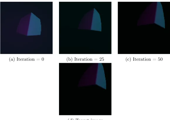
Figure 6-1 demonstrates intermediate renderings of the optimization of a rigid trans-formation of a cube in one orientation to a cube in a different orientation. All images were rendered at a resolution of 200x200. After 50 iterations, the gradient descent
(a) Iteration = 0 (b) Iteration = 25 (c) Iteration = 50
(d) Target image
Figure 6-1: Inferring a Rigid Transform from a Single Image. In this example, we infer the transform from the initialization to the target in under 50 epochs. The 𝜎 parameter used for both images is 1 × 10⁻², and the learning rate was 1 × 10⁻²
Figure 6-2: Loss of Rigid Transform Fitting. After roughly fifty epochs of train-ing, an acceptable transform between the initialization and target cube which mini-mized the MSE between the two images was found.
process manages to align the cube almost perfectly with the final position. The loss and the transform error are shown in figure 6-2.
Learning the rigid transformation between two objects is a simple task which confirms that the attenuation function is properly dispersing gradients.
6.1.2
Multi-View Reconstruction
Multi-view 3D reconstruction from 2D images is a more complex task than rigid trans-form estimation. The multi-view reconstruction example below omits the intensity term in the rendering integral.
21 different views of the target geometry (the Stanford bunny) were used as an input to the reconstruction task (see figure 6-3). Each image was rendered with a 𝜎 of 1 × 10⁻² at a resolution of 200x200. The initialization distance field was a sphere. The model geometry was also rendered at a resolution of 200x200, but instead of using a fixed 𝜎 value, the 𝜎 value decreased from 6 × 10⁻¹ to 1 × 10⁻² during training according to the relation 6.1. The learning rate used for all the multi-view experiments was 1.
𝜎 = 4 × 10
−1
𝑒𝜅*epoch+ 1 × 10⁻²; (6.1)
Gradually decreasing the value of 𝜎 over many epochs of training is similar to coarse-to-fine optimization. Starting with a larger 𝜎 value facilitates optimization be-cause the radius of the attenuation function is much larger (see figure 3-1 for details). Figure 6-4 shows intermediate distance fields and gradients over the course of 40 iterations. The penalty method was used to correct the distance field after each epoch. Figure 6-6 shows the loss and Eikonal penalty term over each epoch of optimization. Figure 6-5 shows a visualization of the optimized distance field at iteration 70.
Figure 6-7 shows the results of another experiment in which a sphere is optimized into a torus over the course of 900 iterations using 20 views of the target geometry at a resolution of 200x200. The value of 𝜎 was fixed at 6 × 10⁻¹ to expedite the process at the cost of reduced resolution.
Figure 6-3: Target Views of Bunny
6.2
Discussion
Our results demonstrate that our differentiable renderer is capable of performing a variety of inverse rendering tasks, such as optimizing a rigid transform based on a single image, or performing 3D reconstruction given multiple views. The 3D recon-struction results demonstrate that our approach can optimize for scenes with different topology than the initialization geometry.
There are several limitations of our approach. To begin with, all of the objects in our scenes share the same material properties. The material properties could be stored in another volume, similar to the learned color and opacity volumes used by Lombardi et al. [24]. Alternatively, a surface parameterization of the signed distance field could be learned, which would enable adaptive level of detail (like the warp field used by Lombardi et al. [24]).
Our method is sensitive to the input hyperparameters, such as the learning rate used by the ADAM optimizer or the value of 𝜎 in the attenuation function (see equa-tion 3.9). Equaequa-tion 6.1 gradually reduces the 𝜎 parameter as a form of coarse-to-fine optimization. At first, greater values of 𝜎 (i.e large radius of the attenuation function) accelerate the optimization process, but inevitably lose detail in the rendered image. Smaller values of 𝜎 slow down the optimization process, but allow for finer details to appear. The rate at which this process occurs, 𝜅, influences the quality of the final
(a) Two rendered perspectives on iterations 0, 10, 20, 30, 40
(b) Gradient visualization for Figure 6-4a
(c) SDF visualization for Figure 6-4a
Figure 6-4: Optimizing a Sphere into a Bunny. In this example, we optimize the geometry of the initialization sphere to the target bunny. While most of the optimization completed in the first ten epochs, the ears and legs continue to extend over the course of the next 40 epochs. The 𝜎 parameter used for the target geometry is 1 × 10⁻² while the fixed 𝜎 parameter for the model is 6 × 10⁻¹, and the learning rate is 1. Figure 6-4b is a visualization of the contributions of each ray (i.e pixel) to the gradient of the distance field. Green corresponds to a negative contribution (i.e carving away) and blue corresponds to a positive contribution (i.e strengthening).
Figure 6-5: Bunny SDF Visualization. This figure shows multiple perspectives of the learned signed distance field of the sphere to bunny optimization at epoch 70. Some incorrect distance values, especially near the ears and tail, are still present. Additionally, a number of smoke-like artifacts are present around the bunny.
(a) Loss (b) Eikonal Penalty
Figure 6-6: Bunny Optimization Loss. Figure 6-6a shows the loss associated with the optimization process and Figure 6-6b shows the Eikonal penalty over each epoch of training. The smoothness of Figure 6-6a is likely due to equation 6.1.
(a) Target Views of Torus
(b) Iteration 500 – side view (c) Iteration 500 – gradient
(d) Iteration 900 – front view (e) Iteration 900 – SDF visualization
Figure 6-7: Optimizing a Sphere into a Torus. In this example, we optimize the geometry of the initialization sphere to the target torus in the course of 900 epochs. The 𝜎 parameter used for the target geometry is 1 × 10⁻²while the fixed 𝜎 parameter for the model is 6 × 10⁻¹, and the learning rate is 1. Figure 6-7c is a visualization of the contributions of each ray (i.e pixel) to the gradient of the distance field. Green corresponds to a negative contribution (i.e carving away) and blue corresponds to a positive contribution (i.e strengthening).
signed distance field. Unfortunately, it is not obvious how to determine the best value of 𝜅, as well as the initial and final values of 𝜎, a priori.
The reconstruction results show a small number of cloud-like artifacts on the periphery of the distance field. It is plausible that these artifacts are the result of the optimizer reaching a local minimum, exacerbated by an insufficient number of viewpoints. Lombardi et al. address this issue by introducing two priors to the reconstruction process [24]. A similar process could be incorporated into our Eikonal penalty (see equation 4.9).
Our differentiable renderer is not designed to run in real-time. The CUDA im-plementation is currently limited by inefficient checkpointing (see section 5.1.1 for an explanation of the checkpointing process). Experimenting with different check-pointing schedules, such as log checkcheck-pointing [10], would reduce memory usage and improve occupancy.
6.3
Future Work
Integrating the volumetric renderer into the redner differentiable renderer [21] is a potential next step of this research. Optimizing scenes which contain a mixture of polygon meshes and signed distance function geometry may be possible. The inclusion of a volume renderer in redner would help create a toolkit of differentiable rendering primitives which could be combined for a variety of inverse-rendering applications. In particular, our approach could be used to construct adversarial examples for neural networks [3]. For example, a neural network may correctly categorize an image of a chair as a chair; however, given some small modification to the geometry or material properties of the chair, this categorization may not hold true. Using a differentiable 3D renderer, one may use gradient descent to minimize the output score associated with the chair class and discover such a modification.
A differentiable volumetric renderer of signed distance fields could be used to perform the same kind of marker-less pose estimation introduced by Rhodin et al. [31]. In particular, a hand or finger tracking application could be a compelling
use-case. A parametric signed distance function model could be used to describe the geometry of the hand which would then be optimized to the camera input using our differentiable renderer, perhaps with additional terms in the loss function to impose soft constraints upon the hand pose. Taylor et al. [35] approached the hand tracking problem by fitting point cloud data from a Microsoft Kinect sensor to a hand model using non-linear gradient-based optimization. Most of the terms in their energy function are soft constraints which could be applicable for a volume-rendering based hand tracker.
A differentiable renderer is a useful tool for any application which endeavors to understand the three-dimensional nature of a rendered image, photograph, or video. We hope that a general-purpose differentiable rendering toolkit will help integrate the well-understood principles of light transport in computer graphics with computer vision and learning approaches.
Bibliography
[1] CUDA C Best Practices Guide. http://docs.nvidia.com/cuda/ cuda-c-best-practices-guide, 2017.
[2] Metashape. https://www.agisoft.com/, 2019.
[3] Anish Athalye, Logan Engstrom, Andrew Ilyas, and Kevin Kwok. Synthesizing robust adversarial examples. arXiv preprint arXiv:1707.07397, 2017.
[4] Jonathan T Barron and Jitendra Malik. Shape, illumination, and reflectance from shading. IEEE transactions on pattern analysis and machine intelligence, 37(8):1670–1687, 2014.
[5] Volker Blanz and Thomas Vetter. A morphable model for the synthesis of 3D faces. In Proceedings of the 26th Annual Conference on Computer Graphics and Interactive Techniques, SIGGRAPH ’99, pages 187–194, New York, NY, USA, 1999. ACM Press/Addison-Wesley Publishing Co.
[6] T. Chan and Wei Zhu. Level set based shape prior segmentation. In 2005 IEEE Computer Society Conference on Computer Vision and Pattern Recogni-tion (CVPR’05), volume 2, pages 1164–1170 vol. 2, June 2005.
[7] SM Ali Eslami, Nicolas Heess, Christopher KI Williams, and John Winn. The shape boltzmann machine: a strong model of object shape. International Journal of Computer Vision, 107(2):155–176, 2014.
[8] Ian J. Goodfellow, Jonathon Shlens, and Christian Szegedy. Explaining and harnessing adversarial examples. CoRR, abs/1412.6572, 2014.
[9] Chris Green. Improved alpha-tested magnification for vector textures and special effects. In ACM SIGGRAPH 2007 courses, pages 9–18. ACM, 2007.
[10] Andreas Griewank. Achieving logarithmic growth of temporal and spatial com-plexity in reverse automatic differentiation. Optimization Methods and software, 1(1):35–54, 1992.
[11] Brian Guenter. Efficient symbolic differentiation for graphics applications. In ACM SIGGRAPH 2007 Papers, SIGGRAPH ’07, New York, NY, USA, 2007. ACM.
[12] Markus Hadwiger, Joe M. Kniss, Christof Rezk-salama, Daniel Weiskopf, and Klaus Engel. Real-time Volume Graphics. A. K. Peters, Ltd., Natick, MA, USA, 2006.
[13] John C Hart. Sphere tracing: A geometric method for the antialiased ray tracing of implicit surfaces. The Visual Computer, 12(10):527–545, 1996.
[14] Wolfram Research, Inc. Mathematica, Version 12.0. Champaign, IL, 2019. [15] Phillip Isola, Jun-Yan Zhu, Tinghui Zhou, and Alexei A Efros. Image-to-image
translation with conditional adversarial networks. In Proceedings of the IEEE conference on computer vision and pattern recognition, pages 1125–1134, 2017. [16] Nima Khademi Kalantari, Ting-Chun Wang, and Ravi Ramamoorthi.
Learning-based view synthesis for light field cameras. ACM Trans. Graph., 35(6):193:1– 193:10, November 2016.
[17] Tero Karras, Timo Aila, Samuli Laine, and Jaakko Lehtinen. Progressive growing of gans for improved quality, stability, and variation. 10 2017.
[18] Hiroharu Kato, Yoshitaka Ushiku, and Tatsuya Harada. Neural 3D mesh ren-derer. In Proceedings of the IEEE Conference on Computer Vision and Pattern Recognition, pages 3907–3916, 2018.
[19] Diederik P. Kingma and Jimmy Ba. Adam: A method for stochastic optimiza-tion. CoRR, abs/1412.6980, 2014.
[20] Jed Lengyel. The convergence of graphics and vision. Computer, 31(7):46–53, 1998.
[21] Tzu-Mao Li, Miika Aittala, Frédo Durand, and Jaakko Lehtinen. Differentiable monte carlo ray tracing through edge sampling. In SIGGRAPH Asia 2018 Tech-nical Papers, page 222. ACM, 2018.
[22] Tzu-Mao Li, Michaël Gharbi, Andrew Adams, Frédo Durand, and Jonathan Ragan-Kelley. Differentiable programming for image processing and deep learn-ing in halide. ACM Transactions on Graphics (TOG), 37(4):139, 2018.
[23] Shichen Liu, Tianye Li, Weikai Chen, and Hao Li. Soft rasterizer: A differentiable renderer for image-based 3D reasoning. The IEEE International Conference on Computer Vision (ICCV), Oct 2019.
[24] Stephen Lombardi, Tomas Simon, Jason Saragih, Gabriel Schwartz, Andreas Lehrmann, and Yaser Sheikh. Neural volumes: Learning dynamic renderable volumes from images. arXiv preprint arXiv:1906.07751, 2019.
[25] Matthew M Loper and Michael J Black. Opendr: An approximate differentiable renderer. In European Conference on Computer Vision, pages 154–169. Springer, 2014.