LIMIT CYCLES STABILITY FOR COMPLEX SYSTEM

HAL Id: hal-01966642

https://hal.archives-ouvertes.fr/hal-01966642

Submitted on 29 Dec 2018

HAL is a multi-disciplinary open access

archive for the deposit and dissemination of

sci-entific research documents, whether they are

pub-lished or not. The documents may come from

teaching and research institutions in France or

abroad, or from public or private research centers.

L’archive ouverte pluridisciplinaire HAL, est

destinée au dépôt et à la diffusion de documents

scientifiques de niveau recherche, publiés ou non,

émanant des établissements d’enseignement et de

recherche français ou étrangers, des laboratoires

publics ou privés.

LIMIT CYCLES STABILITY FOR COMPLEX

SYSTEM

Lala Rajaoarisoa, N. M’Sirdi

To cite this version:

Lala Rajaoarisoa, N. M’Sirdi. LIMIT CYCLES STABILITY FOR COMPLEX SYSTEM. ICINCO

2007, Dec 2007, Anger, France. �hal-01966642�

LIMIT CYCLES STABILITY FOR COMPLEX SYSTEM

Lala H. Rajaoarisoa, Nacer K. M’Sirdi

Laboratory of Systems and Information Sciences LSIS UMR CNRS 6168,

Domaine Universitaire. St Jerome, Av. Escadrille Normandie Niemen, Marseille, France

lala.rajaoarisoa@lsis.org, nacer.msirdi@lsis.org

Keywords: Limit Cycles , Stability, Multiple Lyapunov Function, Hybrid System, Variable Structure System, Discrete

Events System.

Abstract: Limit cycles are common in physical complex systems. However the nonsmooth dynamics of such systems

makes stability analysis difficult. This paper gives an extension of Discrete Events System formalism to show the statibilty of Limit cycles using multiple lyapunov function.

1

INTRODUCTION

Many real systems are characterized by interac-tions between continuous (smooth or none) dynam-ics and discrete events. Such systems are common across a diverse range of application areas. Exam-ples include a robotic assembly (McCarragher96 and al.), manufacturing (Pettersson99) and power system (Hiskens00 and al.).

Dynamics of several physical systems can be well described by use of ordinary differential equations de-spite the fact that some times nonlinearities are intro-duced and can be taken into account. However, there is as of time this class of systems exhibit a periodic behavior. Discrete events, such as saturation limits, can act to trap evolving system state within a con-strained region of state space.

Therefore even when the underlying continuous system are unstable, the discrete events can induce a stable limit set. Limit cycles (periodic behaviour) are created in this way. Limit cycles can be stable (attract-ing), unstable (repelling) or non-stable(saddle). The stability of periodic behaviour can be defined also as the stability of the fixed point.

So, in this paper we want to study the problems of stability of some class of hybrid systems and how to deal with observability and controllability of such systems. Despite an amount of theory and proposed methods to test observability, it seems to be rather dif-ficult to find an optimal way and efficient rules which

cope with some class of hybrid non-linear systems. This is why we have chosen some simple mechani-cal systems with different phases when operating, or commutation of structures (contact and non contact situations).

2

MODEL

2.1

Background

We choose as illustrative example a mass spring sys-tem with a simple structure. But this syssys-tem has a structure which is near to a vehicle one or a jumping robot.

Definition of a class of systems having variable structures, commutations in their dynamic behavior, non linearities (hard or smooth), non stationarity, varying parameters and other non standard features, is difficult to be done in general. So we can restrict our case to some simple situations with known involved physical phenomena.

The discrete events taken into account and the choice of their effect may be driven by some higher level or simply selected according of optimization of some criterion or performance index (Giambiasi02 and al.), (Allur94).

The switchings and commutations often appear abruptly but changes from one representation to

an-other one may be very smooth or not. In anan-other hand we must note also that such systems representation is not unique and differences can appear between the be-havioral representation and physical system descrip-tion or modeling for diagnosis and control.

Discrete Events System (Zeigler76) defines a way to specify systems which states change either upon the reception of an input event or due to the expiration of a time delay.

The system equation can then be written in fol-lowing form:    ˙ x= fmi(x, u,t) mi:{S, I, O,δint,δext,λ,tαi} (1) where:

• x is the set of continuous states of system • u is the set of input controls

• S is the set of sequential states • I is the set of external events • O is the set of internal events

• δint: S→ S is the internal state transition function • δext : S−× I → S+is the external state transition

function

• λ: S→ O is the output function • tαiis the time advance function

2.2

Limit Cycles Analysis

In the sequel, we adopted following definitions to ap-proach the stability in dynamical of the system given by the relation (1) (MSirdi98 and al.). We considered the system behavioural in the vicinity of one cyclic trajectory in the goal to analysis the orbital stability.

Limit Cycles: for a second order system with

state equation defined by ˙χ= f (χ,t), we define a

posi-tive limited set invarying for a boundedness trajectory

χ(t)(kχ(t)k) < µ, ∀t > 0 by:

-= {p ∈ℜn_{,∀ξ>0,∃t}

k such thatkp −χ(tk)k <

ξ,∀k ∈ N} where tk is the time sequencial, with, lim

k→∞tk=∞

Orbital Stability: Trajectory of the system in the

phase planeℜ2_{is an orbit stable if:}

- ∀ξ >0,∃ρ >0 such that kx0− -(z0) < ρ ⇒

in fkx(t) − pk <ξ,∀t > t0with p∈ℜn

Asymptotic Orbital Stability: Trajectory of the

system in the phase planeℜ2 _{is an asypmtotic orbit}

stable if: -kx0− -(.) <ρ⇒

lim

k→∞in fkx(t) − pk = 0

with p∈ℜn

3

System Description

3.1

Mass Spring Model

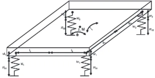
Let us consider the mass-spring system of figure(4), with mass M, stiffness constant k and z0 the

origi-nal length of massless spring. The environment is assumed infinitely rigid: ke >> k. If this is not

the case let kr be the stiffness of the spring and k

the equivalent stiffness of interaction with the ground

(k ∼= krke

kr+ke). The position of the mass M, in a frame

attached to the ground, is noted z. The gravity con-stant is g= 9.81ms−2. Let vd= ˙zd>0 be the lift off

velocity and vc= ˙zc<0 the touch down velocity.

The dynamic interaction with the ground is com-posed by two phases: flying and stance phases [16][17]. This system is composed by interconnec-tionof three subsystems (mass, spring and ground) and energy evolutions are:

Potential (g)→ Kinetic → potential accumulation →

potential restitution→ Kinetic and so on.

We assume the landing without rebounds and no en-ergy loss. Note that the values used in simulations are estimations of equivalent coefficients for out robot SAP [15] (M ∼= 2.6kg; k = 1100). z, M ul1 kl1 kr1 kr2 kl2 zl01 zr01 ur1 zr02 ur2 ul2 zl02 è ¦ l1 l2 d1 d2 z, M ul1 kl1 kr1 kr2 kl2 zl01 zr01 ur1 zr02 ur2 ul2 zl02 è ¦ l1 l2 d1 d2

Figure 1: Mass Spring Model

• Contact Phases. In these phases the controls are

active when the springs are in contact.

- The two springs are in contact: ˙x= f1(x, u,t) t ∈

R+ and x(t) ∈ D1⊂ R4    ˙ x4= ¨z = −_Mkl(zl− zl0− ul) −kr_M(zr− zr0− ur) − g ˙ x5= ¨θ=lkIl(zl− zl0− ul) −lkrI (zr− zr0− ur) ˙ x6= ¨φ=lk_Il(zl− zl0− ul) +lkr_I (zr− zr0− ur) (2) - The right spring is in contact: ˙x= f2(x, u,t) t ∈

R+ and x(t) ∈ D2⊂ R4    ˙ x4= ¨z = −kr_M(zr− zr0− ur) − g ˙ x5= ¨θ= −lkr_I (zr− zr0− ur) ˙ x6= ¨φ=lkr_I (zr− zr0− ur) (3)

- The left spring is in contact: ˙x= f3(x, u,t) t ∈ R+ and x(t) ∈ D3⊂ R4    ˙ x4= ¨z = −k_Ml (zl− zl0− ul) − g ˙ x5= ¨θ=lkIl(zl− zl0− ul) ˙ x6= ¨φ=lk_Il(zl− zl0− ul) (4)

• Flying Phase: ˙x = f4(x, u,t) t ∈ R+ and x(t) ∈

D4⊂ R4          ˙ x1= x3 ˙ x2= x4 ˙ x4= ¨z = −g ˙ x5= ¨θ= 0 ˙ x6= ¨φ= 0 (5)

zr et zl can be expressed in function of z if we

assumeθandφsmall:

     zl1= z − l sinθ− d sinφ= z − lθ− dφ zl2= z + l sinθ− d sinφ= z + lθ− dφ zr1= z + l sinθ− d sinφ= z + lθ− dφ zr2= z + l sinθ+ d sinφ= z + lθ+ dφ

3.2

Switching control and supervisor

model

As we have said above, our system is composed of two sub-system. One hand with continuous state and in other hand discrete behavioural state. For this last, we considerate the following phases (Figure2) :

– All springs are in contact with ground – All springs are in flying phase

– Before Right-hand side Spring is in contact

with ground

– Before Letft-hand side Spring is in contact with

ground

– Back Right-hand side Spring is in contact with

ground

– Back Letft-hand side Spring is in contact with

ground

– Before and Back Right-hand side Spring is in

contact with ground

– Before and Back Left-hand side Spring is in

contact with ground

- The set of the output variables are gotten by the selector element device (Select1 and Select2). These selectors are associated respectively to Contact model and Flight model. Thus, we can write:

−Oc= Select1= Contact model = 1

−Or1C= Select2= Right1Contact model = 2

−Ol1C= Select3= Le f t1Contact model = 3

−Of = Select4= Flight model = 4

−Or2C= Select2= Right2Contact model = 5

−Ol2C= Select3= Le f t2Contact model = 6

−Or1l1C= Select4= Right1Le f t1Contact model = 7

−Or2l2C= Select4= Right2Le f t2Contact model = 8

For this application let us consider the functions

ξr(zr,ur) andξl(zl,ul) as the external state

transi-tion functransi-tion. So we can write:

δext: S−× I → S+=ξτ(zτ,uτ) (6)

withτ= l, r which defined the Left or Right spring

This function can be equal to 0 in the flying phase and 1 when there is contact with the correspond-ing sprcorrespond-ing. ξr(zr,ur) = 1 2(1 − sign(zr− z0− ur)) (7) ξl(zl,ul) = 1 2(1 − sign(zl− z0− ul)) (8) S1 S5 S6 S4 S1 S5 S6 S4 S1 S2 S3 S4 S1 S2 S3 S4 S1 S7 S4 S1 S7 S4 S 1 S8 S 4 S 1 S8 S 4 I(t) O(t)

Figure 2: Discrete Event Device Model

We want give a periodic motion for our system i.e. to damp any rotational motion and maintain hopping along z axis. For obtain this goal, let us consider the following Lyapunov function (energy of the system):

V =1 2˙z 2_{+ gz +} I 2Mθ˙ 2₊ I 2Mφ˙ 2 ₍₉₎ V = VLC+VT(1)+VT(2) (10) whit≡ VLC=1₂˙z2+ gz VT(1)=2MI θ˙2 VT(2)=2MI φ˙2 (11)

Energy is splitted in two parts: VLCthe energy

cor-responding to the desired periodic hopping mo-tion and V_T(.) the transverse motion energy. It is clear that one of this energy has to be regulated to some level and the other must be damped. The right an left control inputs are

       ξr1ur1=1₂¡uLC− uT(1)− uT(2)¢ ξl1ul1=1₂¡uLC+ uT(1)− uT(2)¢ ξr2ur2=1₂¡uLC− uT(1)+ uT(2)¢ ξl2ul2=12¡uLC+ uT(1)+ uT(2)¢ (12)

uT is the control which has to damp transverse

en-ergy VT and then rotional motions. This has as

consequence to keep the system state in the plane

(z, ˙z) withθ= ˙θ= 0 andφ= ˙φ= 0. The uLC has

to stabilise priodic cycle (cyclic motion). The two control inputs uT and uLC have to be applyed in

the time period where the corresponding spring is in contact with ground. This is made by displace-ment of the springs attach points urand ul.

3.3

Convergence and stability of the

periodic motion

The transverse motion and its energy VT have

to be damped. Let us use as Lypunov candidate function V1 V1= 1 2V 2 T(1)+ 1 2V 2 T(2) (13)

Its time derivative is: ˙ V1= VT(1)V˙T(1)+VT(2)V˙T(2) (14) ˙ VT(1)= I M ˙ θ_θ¨ ₍₁₅₎ ˙ VT(2)= I M ˙ φ_φ¨ ₍₁₆₎

using expression (??) and (16), lead:

˙ VT = lk M(ξl(zl− zl0) −ξr(zr− zr0) (17) + (ξrur−ξlul)˙θ+ lk M(ξl(zl− zl0) −ξr(zr− zr0) + (ξrur−ξlul)˙φ

Substitutind controls ξrur, ξlul by equation (12) in

˙ VT,we have: ˙ VT= lk M(ξl(zl− zl0) −ξr(zr− zr0) + uT) ˙θ +lk M(ξl(zl− zl0) −ξr(zr− zr0) + uT) ˙φ (20)

We propose a transverse control input uT as follows:

uT=ξrur−ξlul= −Γ11ψ(VT(1))˙θ−Γ12ψ(VT(2))˙φ

(21)

−ξl(zl− zl0) +ξr(zr− zr0)

ψis a positive function and can be sign or saturation function (21). we then obtain:

˙ VT = − lk MΓ11ψ(VT(1))˙θ 2₋lk MΓ12ψ(VT(2))˙φ 2 ₍₂₂₎ ˙ V1= VT(1)V˙T(1)+VT(2)V˙T(2) (23) = −Γ11VT(1)ψ(VT(1))˙θ2 (24) −Γ12VT(2)ψ(VT(2))˙φ2≤ 0 (25)

V_T(.)V˙_T(.) is negative then the transverse energy VT

converges to zero. We can conclude that

∀ε1>0,∃t1≥ 0, such as | VT|<ε1, ∀t > t1

Convergence of VLC desired reference VLC∗. Let us

choose another Lyapunov candidate function

V2= 1 2V 2 T+ 1 2(VLC−V ∗ LC) 2 (26)

V_LC∗ the constant reference energy is defined at the lft off pont ˙zdor at the maximal desired height zmax:

V_LC∗(0, zd) =

1 2˙z

2

d or VLC∗ (zmax,0) = gzmax

when t > t1we have (VT, ˙VT) = (0, 0), then

˙ V2= (VLC−VLC∗) ˙VLC ∀t > t1 with ˙ VLC= (¨z + g) ˙z ∀t > t1 (27) ˙ VLC= µ −ξl k M(zl− zl0) −ξr k M(zr− zr0) (28) + k M(ξrur+ξlul)˙z (29) ˙ VLC= µ −ξl k M(zl− zl0) −ξr (30) k M(zr− zr0) + k MuLC˙z (31)

we propose as control input :

uLC=ξrur+ξlul= −Γ2ψ(V −VLC∗)˙z (32) +ξl(zl− zl0) +ξr(zr− zr0)

such as the derivative ˙VLCwill be negative:

˙ VLC= − k MΓ2ψ(V −V ∗ LC)˙z2 (33) Then ˙ V2= (VLC−VLC∗ ) ˙VLC (34) = −k MΓ2(VLC−V ∗ LC)ψ(VLC−VLC∗)˙z2≤ 0

The second Lyapunov function ensures global asymp-toticconvergence of the system trajectories z to the or-bitΩ θ(t), ˙θ(t) converge to zero with the following

control:    uT= −Γ11ψ(VT(1))˙θ−Γ12ψ(VT(2))˙φ −ξl(zl− zl0) +ξr(zr− zr0) uLC= −Γ2ψ(V −VLC∗ )˙z +ξl(zl− zl0) +ξr(zr− zr0) (35)

4

EXPERIMENTAL RESULTS

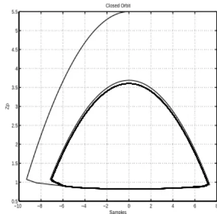
We want just to show firstly whenθ0= 0rad

andφ0= 0rad that our system can respect the

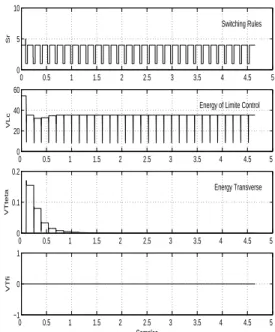
limit cycle that we have imposed with the con-trol considered. These conditions give for the simulation in figure(03) good results with the desired height zm= 3.5m. The figure (04)

il-lustrates the model commutation, here we have just cummutation of model 1 to model 4, the transverse energy VT and the cycle in vertical

direction (VLc goes to its imposed reference)

and the Figure(05) shows the angle θ and φ equal to zero.

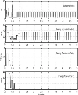
– Second test:

Now we consider thatθ0= 0.5rad,φ0= 0rad.

With the same conditions for simulation fig-ure(06) shows the good results with the desired height zm= 3.5m obtain after few seconds of

simulation, here t= 1.5s. Figure(07) illustrated

the switching model result and the moment that corresponds to the necessary time interval to damp the transverse energy VT and stabilize the

cycle in vertical direction (VLc. The Figure (08)

shows the convergence of the angleθ.

– Third test:

For the sequel, we make one test whose the goal is to show the effectiveness of our supervision

−10 −8 −6 −4 −2 0 2 4 6 8 0.5 1 1.5 2 2.5 3 3.5 4 4.5 5 5.5 Samples Zp Closed Orbit

Figure 3: Cycle limite stable forθ0= 0rad,φ0= 0rad

0 0.5 1 1.5 2 2.5 3 3.5 4 4.5 x 104 0 5 10 Sr Switching Rules 0 0.5 1 1.5 2 2.5 3 3.5 4 4.5 0 20 40 60 VLc

Energy of Limite Control

0 0.5 1 1.5 2 2.5 3 3.5 4 4.5 −1 0 1 VTteta 0 0.5 1 1.5 2 2.5 3 3.5 4 4.5 −1 0 1 Samples VTfi

Energy Transverse Teta

Energy Transverse Fi

Figure 4: Energy of the System M whenθ0= 0rad,φ0=

0rad

and commutation device. In this effect, let us

θ0= 1rad,φ0= 0.5rad. As before, the

simu-lation show us the good results with the desired height in figure(09) and in the Figure (10) we can see one more variation a both, of commu-tation models and the system Energy. The Fig-ure(11) shows the convergence of the angle θ and the angleφafter few seconds of the simu-lation time.

0 0.5 1 1.5 2 2.5 3 3.5 4 4.5 −1 −0.5 0 0.5 1 Teta 0 0.5 1 1.5 2 2.5 3 3.5 4 4.5 −1 −0.5 0 0.5 1 Samples Fi

Stable swing angle of the mass M

Figure 5: Stable swing angle of the mass M whenθ0=

1.5rad, −10 −8 −6 −4 −2 0 2 4 6 8 0.5 1 1.5 2 2.5 3 3.5 4 4.5 5 5.5 Samples Zp Closed Orbit

Figure 6: Cycle limite stable forθ0= 0.5rad,φ0= 0rad

5

CONCLUSION

We propose of this work is to define an approach to identify and then control and supervise such class of complex systems represented by switched mod-els. The system is composed by different sub-modmod-els. Each model switches to another instantaneously when the thresholds that define some operating points or zone, is reached by the application of the external or internal transition function. In the goal to build the best prediction of system outputs, we have to get the best switching and supervision device depending on operating point, the behavior and environment. We have illsutred the observability of this class of system with different phases when operating, or commutation of structures (contact and non contact situations). The presented experimental results emphasize effi-ciency of this approach for modeling, behavior anal-ysis and prediction for such class of complex sys-tems. We have shown, in our first results using this

ap-0 0.5 1 1.5 2 2.5 3 3.5 4 4.5 5 0 5 10 Sr Switching Rules 0 0.5 1 1.5 2 2.5 3 3.5 4 4.5 5 0 20 40 60 VLc

Energy of Limite Control

0 0.5 1 1.5 2 2.5 3 3.5 4 4.5 5 0 0.1 0.2 VTteta 0 0.5 1 1.5 2 2.5 3 3.5 4 4.5 5 −1 0 1 Samples VTfi Energy Transverse

Figure 7: Energy of the System M whenθ0= 0.5rad,φ0=

0rad 0 0.5 1 1.5 2 2.5 3 3.5 4 4.5 5 −0.4 −0.2 0 0.2 0.4 0.6 Teta 0 0.5 1 1.5 2 2.5 3 3.5 4 4.5 5 −1 −0.5 0 0.5 1 Samples Fi

Stable swing angle of the mass M

Figure 8: Stable swing angle of the mass M whenθ0=

0.5rad,φ0= 0rad

proach, an important difference of performance of the prediction regard to the case when using fuzzy logic for estimation and supervision (Duplaix05).

In a future work, this approach will be used for mod-elling a vehicle in the goal to make a diagnosis, fault detection and monitoring. A diagnostic framework on this application will be considered to detect defaults and control the system.

0 0.5 1 1.5 2 2.5 −10 −5 0 5 10 0 1 2 3 4 5 6 Samples Closed Orbit Zp Z

Figure 9: Cycle limite stable forθ0= 1rad,φ0= 0.5rad

0 0.5 1 1.5 2 2.5 3 3.5 4 4.5 5 x 104 0 5 10 Sr Switching Rules 0 0.5 1 1.5 2 2.5 3 3.5 4 4.5 5 0 20 40 60 VLc

Energy of Limite Control

0 0.5 1 1.5 2 2.5 3 3.5 4 4.5 5 0 0.5 1 VTteta 00 0.5 1 1.5 2 2.5 3 3.5 4 4.5 5 0 5 10 15 Samples VTfi

Energy Transverse Teta

Energy Transverse Fi

Figure 10: Energy of the System M whenθ0= 1rad,φ0=

0.5rad

REFERENCES

. Zeigler, Theory of modelling and simulation. John Wiley and Sons, New York, 1976.

. J. McCarragher , G. E. Hovland , Hiden Markov Models as a process monitor in a robotic assembly , International Journal of Robotics research, 1996.

. Pettersson, Analysis and design of hybrid systems, Ph.D. Thesis, DEpertement of signals and systems, Chalmers uni-versity of technology, Goteborg, Sweden, 1999.

. A. Hiskens, M.A. Pai, Hybrid systems view of power system modelling, in Proceedings of the IEEE International Symposium on circuits and Systems, Geneva, Switzerland, May 2000.

. Giambiaisi, N. R. Doboz, E. Ramat, Introduction la mod-lisation vnements discrets, LSIS UMR CNRS 6168, LIL

0 0.5 1 1.5 2 2.5 3 3.5 4 4.5 5 −1 −0.5 0 0.5 1 Teta 0 0.5 1 1.5 2 2.5 3 3.5 4 4.5 5 0 2 4 6 8 10 12 Samples Fi

Stable swing angle of the mass M

Figure 11: Stable swing angle of the mass M whenθ0=

1rad,φ0= 0.5rad

Calais, Rapport interne N LIL-2002-02

. Allur, D. L. Dill, A thoery of timed automata, theoretical computer science, ACM, vol. 126, pp.116-146, N2, 1994 .K.MSirdi, N.Manamani and N.Nadjar- Gauthier Method-ology based on CLC for control of fast legged robots, Intl. Conference on intelligent robots and systems, proceedings of IEEE/RSJ, October 1998.

. Duplaix, J.F. Balmat, F. Lafont, N. Pessel, Data Analysis For Neuro-Fuzzy Model Approach, STIC-LSIS, Universite du Sud Toulon-Var, Sofa 2005.