Online Identification of Last-Mile Throughput Bottlenecks on Home Routers

HAL Id: hal-01401856

https://hal.inria.fr/hal-01401856v2

Submitted on 28 Dec 2016

HAL is a multi-disciplinary open access

archive for the deposit and dissemination of

sci-entific research documents, whether they are

pub-lished or not. The documents may come from

teaching and research institutions in France or

abroad, or from public or private research centers.

L’archive ouverte pluridisciplinaire HAL, est

destinée au dépôt et à la diffusion de documents

scientifiques de niveau recherche, publiés ou non,

émanant des établissements d’enseignement et de

recherche français ou étrangers, des laboratoires

publics ou privés.

Online Identification of Last-Mile Throughput

Bottlenecks on Home Routers

Michele Pittoni

To cite this version:

Michele Pittoni. Online Identification of Last-Mile Throughput Bottlenecks on Home Routers.

Net-working and Internet Architecture [cs.NI]. 2016. �hal-01401856v2�

Online Identification of Last-Mile Throughput Bottlenecks

on Home Routers

Michele Pittoni

Supervisors: Renata Teixeira

_{, Prometh ´ee Spathis}

Advisors: Anna-Kaisa Pietilainen

_{, Srikanth Sundaresan}

_{, Nick Feamster}

Abstract

We develop a system that runs online on commodity home routers to locate last-mile throughput bottlenecks to the home wireless network or the access ISP. Pinpointing whether the home wireless or the access ISP bottlenecks Internet through-put is valuable for home users who want to better troubleshoot their Internet experience; for access ISPs that receive numer-ous calls from frustrated home customers; and for informing the debate on regulating the residential broadband market. Developing such a system is challenging because commodity home routers have limited resources. The main contribution of this thesis is to develop a last-mile throughput bottleneck detection algorithm that relies solely on lightweight metrics available in commodity home routers. Our evaluation shows that our system accurately locates last-mile bottlenecks on commodity home routers with little performance degradation.

1 Introduction

With the availability of cheap broadband connectivity, Inter-net access from the home is ubiquitous. Modern households host many networked devices, ranging from personal devices such as laptops and smartphones to printers, media centers, and a number of other Internet of Things (IoT) devices. These devices often connect with each other and to the Internet via a wireless home network; this connectivity has become an important part of the “Internet experience” [24,32]. Unfor-tunately, home users have few means to identify when their home network bottlenecks their Internet performance, and hence often attribute poor performance to the access ISP. Ac-cess ISPs are in no better position to determine the cause of performance bottlenecks in the last mile, and yet their hot-line must answer numerous calls from unsatisfied customers. Tools for correctly pinpointing whether the home wireless or the access ISP bottlenecks Internet throughput are valuable not only to home users and ISPs, but also to inform the wider debate on regulating the residential broadband market.

In this paper, we develop a system to locate last-mile throughput bottlenecks—which we define as throughput bot-tlenecks either in the access ISP or in the customer’s home.

Clearly, throughput bottlenecks may happen elsewhere (e.g., at peering interconnects [19]). We focus on bottlenecks that are close to users as these more likely affect all of a user’s traffic and users can take direct actions to remedy them.

Last-mile throughput bottlenecks are difficult to identify, for two reasons. First, ISPs lack tools that run within the customer premise, which is necessary to accurately identify last-mile bottlenecks that are caused by the home network. Some tech-savvy home users can run a set of tools (as we dis-cuss in more detail in §8) to help identify last-mile throughput bottlenecks in an ad-hoc fashion, but this ad-hoc procedure is too complex for many home users [12]. Second, through-put bottlenecks are often intermittent, because they depend on the interaction among user traffic, wireless quality of the different devices in the home network, and the access link performance. As a result, single tests will likely fail to capture many bottlenecks that affect user experience. A solution that runs continuously is key to identify last-mile bottlenecks.

To address these challenges, our system runs directly on commodity home routers. The home router is between the home and the access network and hence is ideally placed to locate last-mile bottlenecks. The home router is typically al-ways on, thus permitting continuous monitoring. We improve on previous work [32] which developed a proof-of-concept algorithm, called HoA (for Home or Access), that ran offline on a server to locate last-mile downstream throughput bottle-necks based on the analysis of packet traces collected from home routers. Our attempts to run HoA online on commodity home routers, however, revealed the challenges with perform-ing per-packet analysis on such resource-constrained devices (§2).

The main contribution of this paper is a last-mile through-put bottleneck location algorithm that runs online in commod-ity home routers. We design an access bottleneck detector based on lightweight pings of the access link (§4), and a wireless bottleneck detector based on a model of wireless capacity using metrics that are easily available in commodity home routers such as the wireless physical rate and the count of packets/bytes transmitted (§5). We evaluate the accuracy

of our detectors using controlled experiments (described in §3), and show that we can detect throughput bottlenecks with more than 93% true positive rate and less than 8% false pos-itive rate. Our performance evaluation in §6shows that our algorithm runs online with less than 30% load average on a Netgear router. Finally, we implement our detectors on a production system (§7) and demonstrate an integration with data storage and a user interface.

2 Design Constraints and Choices

In this work we aim to design a throughput bottleneck de-tector for the last mile that has the ability to distinguish be-tween access-link and wireless bottlenecks, that operates with minimal network and system overhead, and with minimal disruption to the end user. Our goal narrows down potential design choices and introduces certain constraints, which we list below.

Design choice: The detector must be located inside the home. To identify throughput bottlenecks in the home wire-less or the access network, we need a vantage point inside the home network. This is because other vantage points typi-cally do not get a view inside the home network. A vantage point in the access ISP, for instance, may be able to detect that traffic is being bottlenecked somewhere in the end-to-end path (for instance, using a tool such as T-RAT [33]), but it will be unable to identify that the last mile is the cause, let alone localize it to the access link or the home wireless net-work. Inside the home network, end clients have a view of the wireless network, but not a direct view of the access link, or even a full view of the wireless network; it may not be able to observe traffic between the home router and other clients in the network. The home router, on the other hand, is the ideal vantage point for locating last-mile bottlenecks as it sits in between the home wireless and the access network and hence can directly measure the performance of each network inde-pendently. Moreover, the home router is always on allowing for the identification of intermittent bottlenecks.

Design constraint: The detector must introduce minimal overhead. The system should not disrupt users. This implies that we must avoid introducing too much traffic in either the access link or the home wireless. This rules out conceptu-ally the simplest detector, that would simply run an active throughput test from the router to some well-connected server in the Internet and to devices within the home and compare the two measurements. Such tests introduce high overhead that is tolerable in one-shot tests, but not continuously. Since wireless conditions are highly variable, the detector would need to run continuously. Probing devices in the home wire-less is also problematic. Not only might probe traffic interfere with user traffic, or even change the wireless network itself by introducing side-effects such as contention, but answering to these probes may drain device battery. Finally, given our system is running on the home router, we must also avoid

overloading the router’s CPU, which could lead to drops in user’s traffic.

Design constraint: Passive packet capture is not feasible. Since active throughput measurements are not viable, an-other natural approach is to passively observe user’s traffic as it crosses the router, as in HoA [32], which examines per-packet arrival rates and computes per-flow TCP metrics to locate last-mile downstream throughput bottlenecks. The ex-isting implementation of HoA collects packet headers on the router, but offloads actual bottleneck identification to a server. This offline approach is feasible in a small-scale deployment for research purposes, but not as a large-scale operational solution due the volume of data, and also due to privacy con-cerns. Unfortunately, our attempts to run HoA online on the router have failed mainly because of the overhead of analyz-ing each packet online. Our study of the fraction of dropped packets when we run tcpdump on a TP-Link WDR3600 access point as we vary the traffic load illustrate this prob-lem. We run tcpdump in two modes: “save” refers to only storing the packets in memory (e.g. tcpdump -w); whereas “parse” refers to the case where tcpdump parses the headers with no other per-packet computation (when omitting the -w flag). We see that using tcpdump to only write packets as in HoA’s implementation causes almost no drops, but when we parse packets in the router we start seeing approximately 10% packet drops at 30 Mbps. This rate increases to 80% at 70 Mbps. High rates of packet drops will make the system unreliable at identifying bottlenecks at higher speed links. Design choice: Lightweight active and passive metrics at the wireless router. These design constraints lead us to two types of lightweight measurements. First, we consider lightweight active measurements, for example, low frequency RTT measurements that should not disrupt users. Second, we consider metrics available by polling the router operating system. Most commodity routers report a number of statistics such as the number of bytes/packets transmitted and received, queueing statistics, and wireless quality metrics (such as PHY rate, RSSI, frame delivery ratio). We will discuss the specific metrics we use for detecting access bottlenecks and wireless bottlenecks in §4and §5, respectively. In the next section we explain the experimental setup we use to train and test these detectors.

3 Experiment Setup

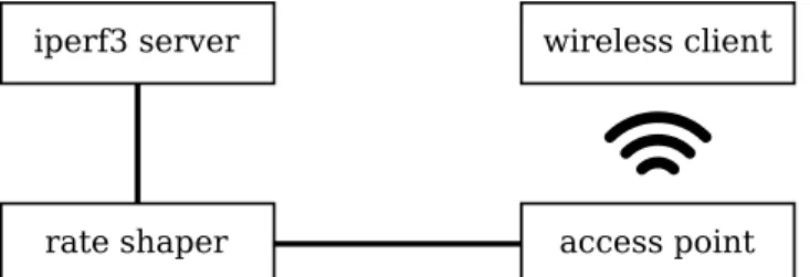
We develop and test our algorithm using a simple testbed, shown in Figure1, to recreate different access link and wire-less quality scenarios. Our testbed consists of two TP-Link WDR3600 access points, a test server, and a Mac laptop. The access points have a 560 MHz MIPS CPU, 128 MiB of RAM, and two wireless interfaces (2.4 GHz and 5 GHz). Both routers run version 15.05 of the OpenWRT firmware. We connect one access point downstream of the other over an ethernet cable; the downstream access point acts as wire-less router, while the upstream access point acts as a traffic shaper to emulate various access link scenarios. We connect

the test server to the upstream server via a Gigabit Ethernet switch. Finally, we connect the Mac laptop over wireless to the downstream access point.

We conduct all our experiments over 802.11n. Although the access points support both 2.4GHz and 5GHz, we use only the 5 GHz band to limit the amount of interference from external sources. We create a variety of wireless scenarios that capture a range of performance ranging from poor to excellent. We do so by moving the client between different rooms, at various distances from the access point, as well as by creating interference. To add interference, we add a second client that sends constant bitrate UDP traffic at 100 Mbps to a separate access point on the same channel that the testbed was using. Using these methods we achieve a range of wireless capacities ranging from less than 20 Mbps to almost 100 Mbps. We test both 20 MHz and 40 Mhz channels; in the latter case, though the maximum (theoretical) capacity is 300 Mbps, the access point itself becomes a bottleneck at about 100 Mbps. We note here that these numbers are approximate, and reveal only a general notion of the quality of the wireless; this is because of the inherent variability associated with wireless network performance.

For the access link, we test different levels of throughput limitations, ranging from 10 to 90 Mbps, by controlling the kernel queuing disciplines on the shaper with tc.

In total, our experiments span 15 scenarios for a total of more than 7 hours of runtime. For each scenario, we test the throughput by sending TCP traffic from the server to the client with iperf. We test both a single flow and multiple parallel flows, with long (5 minutes) and short (30 s) runs. We label each scenario as either access bottleneck or wireless bottleneck based on the prior measurement of the wireless link capacity, and on the access throughput limit set in the shaper.

iperf3 server

rate shaper access point wireless client

Figure 1: Diagram of the experiment testbed

4 Access Bottleneck Detection

In this section, we identify, tune, and validate metrics to detect upstream and downstream bottlenecks in the access-link. We show using extensive controlled experiments that lightweight metrics suffice to detect such bottlenecks with high accuracy.

4.1

Metrics

In §2, we discussed the need for lightweight metrics, and how that rules out active throughput tests. Instead, we identify an intuitive property of bottlenecked links that we can exploit:

increased packet queueing at the bottleneck link buffer. An obvious way to exploit this metric would be to poll the router for queueing statistics to directly identify the presence of queues. The problem with this is that it only works to detect upstream bottlenecks and in cases where the access point is also the modem. In many setups the modem/router and the AP are physically separate devices. In such cases the queue will not increase in the AP if the access link is the bottleneck. We instead use the result of queue buildup: increased queueing delay at the bottleneck link. This principle has been used in congestion control protocols, especially those aimed at low priority traffic (e.g., LEDBAT). It has also been confirmed by studies that have observed home network per-formance from home routers [30]. In our case, we want to isolate the delay of the last mile link. To do so, we identify the first hop inside the ISP’s network and probe it with ping. In this way, the ping packets traverse the access link in both directions and pass through the queues at both ends. Assum-ing FIFO queuAssum-ing, the round-trip time (RTT) is proportional to the sum of the queue lengths. These measurements, in addition to being lightweight, will also capture both upstream and downstream bottlenecks. A few samples during a bottle-neck episode will typically suffice to indicate the presence of a bottleneck.

4.2

Detection Algorithm

The access bottleneck detector keeps an estimate of the min-imum and maxmin-imum RTT observed on the access link (re-spectively, dminand dmax) and compares each new sample

to those values. We consider samples that are higher than a threshold as positive. The detector periodically decides whether there was an access bottleneck based on the ratio of positive samples in the last period.

Intuitively, dmin corresponds to probe propagation delay

plus transmission delay with no queuing delay, whereas dmax

captures the probe delay when buffers are full, so maximum queueing. We estimate dminbased on the minimum measured

RTT over a moving window, and dmaxbased on the maximum

RTT over the same window. We pick a long enough window to increase our chances of encountering both queues empty and full during the window; yet, if the window is too long underlying conditions might change. In our algorithm, we use a window of one hour.

Given an estimation period, T , at time t the detector con-siders the set of samples collected in the interval (t − T,t], denoted SA(t). We identify the set of positive samples as

follows.

PA(t) = {s ∈ SA(t)|s > dmin+ (dmax− dmin) · δA} , (1)

where s is a measured RTT and 0 < δA< 1 is a threshold.

We detect an access bottleneck at time t if the fraction of positive samples is higher than a predefined threshold ρA:

|PA(t)|

0.0

0.1

0.2

0.3

0.4

0.5

False Positives

0.5

0.6

0.7

0.8

0.9

1.0

True Positives

0.00

0.05

0.10

0.90

0.95

1.00

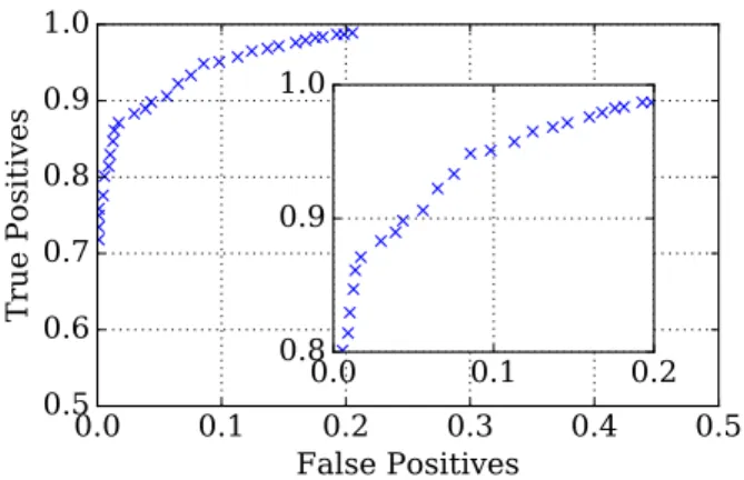
Figure 2: Receiver operating characteristic for access link bottle-neck detection.

The access bottleneck detector relies on four parameters: the estimation period, T , the sampling rate, rA, and the

thresh-olds, δAand ρA. Our goal is to select T short enough to

capture traffic bursts that will trigger network congestion. At the same time, we must have enough samples during T to run access bottleneck detection. If T is too small the rate rA

must increase. As we will discuss in §5, practical limitations with capturing the wireless statistics prevent us from setting intervals shorter than 10 seconds and we must have the same estimation interval for the access and wireless bottleneck de-tectors, so we set T = 10 seconds for both detectors. We pick rA= 10 samples/second, which leads to less than 10 Kbps of

probing bandwidth—low enough not to overload even low capacity access links—and yet gives us 100 RTT samples in each interval. We discuss the selection of the δAand ρAin the

following section.

4.3

Accuracy

We tested the accuracy of the access link detector for differ-ent values of δAand ρA, using the data from our controlled

experiments. Figure2shows the receiver operating charac-teristic (ROC) curve for the detector with δA∈ [0.1, 0.98]

and ρA∈ [0.1, 0.9]. The accuracy remains high over a wide

range of parameters. We must stress that these results are achieved in a very controlled environment, where random variation of the access link delay were unlikely. Nonethe-less, the wide range of parameter values that produce a good accuracy confirms the robustness of the metric. In our ex-periments, we found that the values δA= 0.24 and ρA= 0.5

gave the best trade-off between true positives (99%) and false positives (1%).

4.4

Limitations and improvements

As previously stated, the access bottleneck detector is based on the idea of proportionality between the queue length and the queuing delay. This only strictly holds in the case of FIFO queues with a drop-tail policy. Nevertheless, the detector still functions with queuing algorithms that employ a probabilistic drop policy. We ran experiments with the CoDel active queue

management algorithm [21] and we found no significant dif-ferences in the behaviour and accuracy of the detector. This is explained by the fact that it reacts to any increase over the baseline latency and no queuing algorithm can eliminate this.

A notable exception is the usage of multiple queues, or other mechanisms that treat probe traffic differently from user traffic at the queuing level. This is, for example, the case of stochastic fair queuing (SFQ), where each traffic flow is assigned to a queue based on parameters such as the IP protocol, IP source and destination address and port. In this situation, the user traffic might encounter significant queuing while the probe packets might be assigned an otherwise empty queue. The obvious solution to this scenario is to estimate the latency based on the user traffic instead of dedicated probes. We explained in §2why per-packet analysis and flow tracking are not feasible with our constraints. An alternative might rely on sending probe traffic that mimics the features of user traffic.

As for the real-world impact of these issues, we are not aware of any type of access link that uses SFQ at the mo-ment. Discussion with industry members revealed that net-work equipment vendors are considering implementing SFQ on cable access on the operator side (for downstream traffic).

5 Wireless Bottleneck Detection

In this section, we develop a lightweight metric that is based on aggregate metrics of passive traffic, and similar to the access link metric, show that it performs with high accuracy in detecting wireless throughput bottlenecks.

5.1

Metrics

Our goal is to avoid the overhead associated with wireless frame capture and processing. The HoA tool relies on com-puting the RTT over TCP in the LAN network, i.e., between the router and clients, to infer the presence of queueing, and therefore, the presence of bottlenecks. However, this involves packet captures and heavy processing to maintain flow state. While active RTT measurements to clients in the network is an option, it might drain device battery as they must wake up to answer to probes. Active measurements also might not be representative of wireless state encountered by users’ traffic, as we discuss in §2. We instead poll the wireless driver (ath9k in our case) to obtain metrics that map to link quality. We then feed these metrics to a model that estimates wireless link capacity. We note that the estimated capacity relies on statis-tics that are obtained from the driver based on user traffic, and are therefore likely to reflect actual performance that users get. Our metrics, which we list below, are simple to obtain and are available in most drivers.

We use our estimate of wireless capacity with the achieved throughput to detect the presence of a bottleneck. Since wire-less capacity varies across different clients connected to an access point, we poll the driver for the metrics related to each client. The specific metrics we choose are the physical layer (PHY) bitrate of the last frame sent to the client, frame deliv-ery ratio (which captures the fraction of frames successfully

delivered to the client), and the total number of bytes sent. We also collect non client-specific metrics, such as the fraction of time during which the access point sensed that the channel was busy.

With these metrics, we can estimate the wireless link ca-pacity by using a state of the art model [14]. The model was developed to give an upper bound on capacity for UDP traffic. It starts by computing the maximum number of maximum-size frames that can be aggregated at the link layer, given a PHY bitrate P and the duration of a transmission opportu-nity. Then, it estimates the instantaneous link capacity for P, multiplying the number of aggregated frames by the size of a maximum-size UDP packet and then dividing by the delay to transmit the set of aggregated frames at rate P. Finally, it estimates the link capacity for a period, T , as the average of the instantaneous capacities for the sampled PHY rates in the period times the corresponding frame delivery ratio. We make two modifications to this model. First, we adapted it for TCP traffic, factoring in the increased overhead due to TCP acknowledgments as further discussed in §5.4. Second, we re-move the highest 10% PHY rate samples for each estimation period. The Minstrel rate adaptation algorithm used in our access point sends 10% of “look around” frames by default to test if the medium improved [20], which were causing the model to overestimate the link capacity.

5.2

Detection Algorithm

The wireless bottleneck detection algorithm consists of a sim-ple comparison between the estimated wireless link capacity and the achieved throughput. We compute the latter from the device byte counters over time.

Similar to the access bottleneck detector, there is an estima-tion period T and the detector makes a decision based on the samples collected during the previous period. Let LC(t, c) be the estimated wireless link capacity for client, c, and tput(t, c) the observed throughput over the time interval (t − T,t] for c. The detector flags that c is experiencing a wireless bottleneck at time t if the following test holds.

LC(t, c) − tput(t, c)

LC(t, c) < δW, (3) where 0 < δW < 1 is a threshold.

The wireless bottleneck detector relies on three parame-ters: the estimation period, T , the sampling rate, rW, and the

threshold, δW. The capacity model we use recommends

hav-ing at least 30 samples per estimation period, and we found that polling the router more often than three times per sec-ond had significant impact on performance. The CPU load increases linearly as we increase the sampling rate, until we reach three samples per second when CPU load increases ex-ponentially. Moreover, experiments have shown that, even in a very controlled environment such as an anechoic chamber, the interaction between the AP rate adaptation algorithm and the MAC layer creates variations of the link capacity and the throughput on timescales of less than 30 seconds: we want to

0.0

0.1

0.2

0.3

0.4

0.5

False Positives

0.5

0.6

0.7

0.8

0.9

1.0

True Positives

0.0

0.1

0.2

0.8

0.9

1.0

Figure 3: Receiver operating characteristic for wireless bottleneck detection.

choose an estimation window that ignores these fluctuations. Hence, we set rW = 3 samples/second and T = 10 seconds.

We discuss the setting of δW next.

5.3

Accuracy

We use the data from our controlled experiments to evaluate the accuracy of the wireless bottleneck detector. Figure3

shows the ROC curve for the wireless bottleneck detector with δW ∈ [0.2, 0.49]. We test relatively large values of δW

because the estimated capacity is an upper bound on the available bandwidth. In reality, we found that the achieved throughput is lower, for example due to TCP dynamics. The δW parameter compensates for this overestimation.

As can be seen in Figure3, the accuracy of this detector is not as good the access link detector. This can be partly attributed to imprecise capacity estimations and partly to the difficulty of achieving the theoretical available throughput. We selected δW= 0.36, which gives a true positive ratio above

93% and a false positive ratio below 8%, as the threshold for this detector.

5.4

Limitations and improvements

As shown above, the wireless bottleneck detector is not as accurate as the one for the access link, although still valuable in practical terms. Moreover, the difference between the throughput and the capacity is always substantial, leading to the use of a large threshold. In the following paragraphs, we describe some of the causes of these phenomena.

Dynamics of TCP traffic. The original Wi-Fi link capacity model [14], applies to UDP traffic and assumes that the client is not transmitting anything except 802.11 control frames (i.e. ACK, CTS if applicable). In the case of TCP traffic, this is obviously not true because of TCP acknowledgments: despite being very small compared to the respective data segments, their impact can be significant due to the shared, half-duplex nature of the wireless media and the overhead of the 802.11

0

4

8 12 16 20 24 28 32

Maximum A-MPDU size

0

2

4

6

8

10

Airtime utilization (ms)

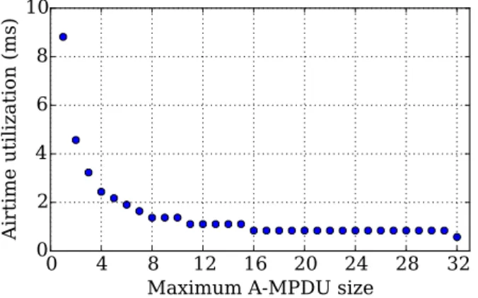
Figure 4: Airtime utilization of 32 TCP ACKs with different A-MPDU sizes.

protocol. Moreover, 802.11n frame aggregation makes this impact difficult to predict.

TCP ACKs and A-MPDUs. The time needed to transmit a certain amount of data, split in a fixed amount of packets, depends on how the MAC layer aggregates those packets in one or more A-MPDUs. Taking pure TCP ACKs as an example, with a layer 3 packet size of 40 bytes, and assuming a fixed PHY rate of 65 Mbps, it takes 573.5 µs to transmit 32 ACKs as a single A-MPDU, 839 µs to send them in two A-MPDUs of size 16 and up to 8816 µs to send them as 32 single 802.11 frames, as can be seen in Figure4. This calculation considers the overhead of the PHY and MAC layers, including inter-frame spacing and control frames.

We use a heuristic to account for the impact of TCP ACKs on the link capacity. Owing to the Nagle algorithm—which we assume to be active for connections that transmit bulk data—we consider the number of ACKs to be half that of data segments, computed by dividing the bytes transmitted by the maximum segment size. We take the average A-MPDU size to be 16, or half of the maximum. This is a very optimistic assumption and leads to a significant overestimation of the capacity, but we reason that the link capacity only represents an upper bound. One factor that heavily influences the impact of TCP ACKs is the number of parallel TCP connections that are used. We observed empirically, by analyzing wireless traffic captures, that by using parallel streams we obtain larger A-MPDU sizes for the ACK traffic. This is due to the fact that large A-MPDU sizes are only used if there are enough packets to be transmitted: with a single connection, it is likely that only a few ACKs will be queued at the client.

Using airtime to estimate ACK traffic. An alternative ap-proach that we explored after the controlled experiments were run is to estimate the impact of ACK traffic by looking at the measured airtime that the AP reports as being spent on receiving traffic. Assuming no other traffic is present, the RX airtime measure can be used directly to adjust the link capacity. This approach has some unfortunate side effects. Firstly, it makes the link capacity vary depending on the

pres-ence of traffic, while it should be only dependent on the link conditions. Furthermore, the A-MPDU size depends on how much the channel is saturated.

Consider a situation where the channel is relatively empty and there are many opportunities to transmit. The client will be able to send ACKs as they are produced by the TCP stack without queuing them, thus preventing the use of large A-MPDUs and occupying a relatively large fraction of time. On the other hand, if transmission opportunities are scarce, frame aggregation allows to “squeeze” the ACKs and use a shorter time by aggregating them. This observation implies that the approach of bonding the link capacity to the measure of RX airtime will lead to an elastic channel, making it much more difficult to identify a bottleneck.

Multiple clients. When multiple clients are downloading content at the same time, the AP implementation decides how the bandwidth should be distributed. Our algorithm does not take into account the possibility of multiple clients and computes the link capacity assuming only one client receives traffic.

In order to overcome this limitation, we ran preliminary experiments to better understand the behaviour of the system. With two similar clients, we ran simultaneous iperf3 tests: we initially positioned both clients close to the AP, then we moved one of the clients in a different room to degrade the wireless link. In both cases, each of the clients reached ap-proximately half of its predicted link capacity. This provides evidence that the AP is dividing the bandwidth between the two clients in terms of airtime utilization rather than actual throughput: if throughput fairness was the goal, more air-time would be dedicated to the client with worse link quality and it would obtain more than half of its link capacity, and vice-versa.

We propose to use a local contention factor C(c,t) to adjust the link capacity estimation accounting for multiple clients with simultaneous activity. This factor corresponds to the ratio of airtime used by a client over the total airtime used by all the clients. It is possible to derive the airtime used by a client by dividing its throughput by the average bitrate:

C(c,t) = tput(c,t)/avgphy(c,t) ∑i∈Ktput(i,t)/avgphy(i,t)

(4) Then, for clients with a positive throughput, the local con-tention factor can be used to refine the link capacity calcula-tion:

LC0(c,t) = LC(c,t) ·C(c,t) (5) Clients with no throughput (or throughput lower than a threshold) should be treated differently to avoid computing an unreasonably low link capacity for them. We have not tested this approach with controlled experiments due to lack of time. Client differences. We ran our controlled experiments with two Mac laptops, a 2012 MacBook Air and a 2015 MacBook. The two laptops were used interchangeably despite not being

identical, depending on their availability at the lab. Both lap-tops had 802.11n Wi-Fi interfaces with 2x2 MIMO, but only one of them supported space-time block coding, a feature that provides more reliable radio communication especially with difficult channel conditions. Other differences may in-clude the antenna design. As a result, we observed a different throughput in similar situations, leading to the use of a thresh-old δW that was a compromise between the behaviours of the

two clients.

In a realistic deployment, having a single threshold for all the clients would be a considerable practical advantage, and we chose to test this scenario. We would still like to underline that a per-client threshold might improve the accuracy of the detector.

6 Evaluation

In this section, we first evaluate the accuracy of our system when compared with the state of the art, HoA [32], using the data from our controlled experiments. Then, we deploy our system in BISmark routers to evaluate its performance overhead in practice.

Comparison with HoA. We apply the HoA detectors on the same set of controlled experiments we used to evaluate the accuracy of our system. Originally, HoA made a decision every second on the access link bottlenecks and one decision per flow on the wireless bottleneck. To make our comparison easier, we apply HoA to detect bottlenecks every 10 seconds as we do with our system.

HoA considers a threshold Tcv= 0.8 on the coefficient of

variation cv of packet inter-arrival times to detect access-link bottlenecks. In our experiments, we tested various thresholds and achieved true positive rate higher than 95% and false positive rate lower than 5%, in the range between 0.7 and 1.8. The best trade-off is when set Tcv= 1.4, which achieves 99%

true positives and 2% false positives. Our detector achieves the same true positive rate with only slightly better false positive rate of 1% (in §4.3).

The wireless bottleneck detector relies on the average RTT inside the home network (between the access point and the client). The original HoA threshold on the home RTT, Tτ,

was 15 ms. In our experiments, however, we achieve only 90% true positive rate with this threshold setting; values in the range [8, 11] ms were better with more than 95% true positives and less than 5% false positives. With this setting, HoA’s wireless bottleneck detector outperforms our detector (which achieves 93% true positive for 8% false positive). Still, the accuracy of our wireless detector is good to be used in practice. We are investigating ways of integrating lightweight pings when we detect traffic from a client to improve the accuracy of our wireless detector.

BISmark Deployment. To evaluate the performance of our system in practice, we deployed a preliminary version of it on 11 devices of the BISmark [29] platform. The devices are Netgear WNDR3700/3800 routers, with a 450 MHz proces-sor, two radio interfaces (2.4 GHz and 5 GHz), and either

0.0 0.2 0.4 0.6 0.8 1.0 1.2 1.4 1.6 1.8 2.0

Load average

0.0

0.2

0.4

0.6

0.8

1.0

Cumulative frequency

Before deployment

After deployment

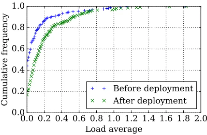
Figure 5: Distribution of the load average on BISmark routers before and after the deployment

128 MiB or 64 MiB of RAM depending on the model. They run OpenWRT version 12.09 with the ath9k driver. This preliminary implementation was written in Lua, a scripting language, and uses command line utilities to poll the oper-ating system. So we are evaluoper-ating a worst-case scenario as a native version, using C to communicate directly with the kernel, would further reduce the overhead.

We examine the load average as reported by the operating system before and after we deploy our system. BISmark col-lects the load average, which is an exponentially weighted moving average with factor e and window sizes of 1, 5, and 15 minutes, once per hour. Figure5shows the distribution of the load average considering a 1-minute window for one day of measurements before and one day after we started our system. The results for 5- and 15-minute windows showed similar trends. As expected, we observe an increase in the system load after we deploy our system. When we average the load for each router over the day before and then after, we see that the average load increase across routers was approximately 9%. This increase is moderate and can be reduced with a na-tive implementation. The vast majority of measurements have load average below 30% even after we deploy our system.

7 System implementation

After evaluating the accuracy and feasibility of our approach, we develop a full system implementation based on the Per-sonal Information Hub (PIH) from the User-Centric Network-ing project [1]. The system consists of two data collectors running on the gateway, the PIH data storage component, and a web interface that displays the results to the user, as displayed in Figure6.

7.1

Wireless data collector

We initially developed the wireless data connector using the scripting language Lua to invoke the iw command line pro-gram for every sample. We found that the overhead of creating a new process multiple times per second was imposing a limit on the sampling rate, as well as some system load as shown in the previous section.

Figure 6: System architecture, including the PIH from the User-Centric Networking project.

For the full system implementation, we decided to port the wireless data collector to C and use the Netlink library instead of the iw program. The Netlink library is used to communicate with the Linux kernel through the Netlink pro-tocol, an inter-process communication mechanism. Notably, the wireless subsystem of the Linux kernel exposes many relevant metrics through Netlink.

The wireless data collector outputs two sets of results to configurable locations on the file system. The first set consists of all the samples in their raw form, and is used primarily for troubleshooting and offline analysis. The second set includes aggregates such as the average PHY rate and the change in packet counters over an interval of 10 seconds. It also includes the throughput and estimated link capacity over the same interval.

7.2

Access link data collector

We use the liboping library to ping the default gateway according to the sampling rate explained in Section4. The collector outputs, to a configurable location on the file sys-tem, aggregate results every 10 seconds, consisting of the maximum, minimum and median RTT for the interval, the IP address of the destination of the pings, and a timestamp.

7.3

Personal Information Hub

The PIH, developed at the University of Cambridge, is a central component of the User-Centric Networking project. It is designed to provide a mechanism for users to have full control of the personal information produced by a variety of sensors and collectors in their home, and enable them to give access to subsets of the data to third parties that offer valuable services.

In our system, we upload the results from the two collectors to the PIH using a simple shell script running on the gateway.

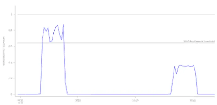
Figure 7: Screenshot of the wireless bottleneck graph in the web UI. The first part shows a wireless bottleneck (utilization over the threshold), while the second part shows an access link bottleneck.

The script polls the directories where the collectors output the results and uploads each file to the PIH via HTTP before deleting it.

The PIH offers an HTTP API for both uploading and downloading the data. The application can upload a JSON file to any URL, including any number of components (e.g. /a/b/c.json). The new file will be created even if some of the components do not exist yet. If the file already exists, it will be simply overwritten. After uploading a file, it can be retrieved at the same URL. There are also two endpoints for each path components: /a/list returns a list of files in directory a, while /a/all returns all the files concatenated as a single JSON object.

We designed the URL structure to provide a limited support for time range queries, which are very useful for displaying time series. We name each file with its time stamp (in seconds since the Unix epoch), and we upload it to a directory obtained by dividing the time stamp by 600 and keeping the integer part. Each directory contains 600 seconds (10 minutes) of results, which is an adequate granularity for our display queries.

7.4

Web-based User Interface

The UI consist of a web page which is served from the PIH itself and uses AJAX to load and refresh the data dynamically. The web page implements the detector logic, rather than the gateway: we did this choice because it is easier to update than the code running on the gateway, and we went to be able to tweak the detectors if needed.

The page presents to the user a plot for the wireless link and one for the access link (other plots, unrelated to our work, are also shown). The wireless plot (Figure7) presents the link utilization over time as the inverse of the left-hand side of equation3, on a scale from 0 to 1. The bottleneck threshold is 1 − δW. The access plot (Figure8) shows the

median RTT over time, on a 0 to 1 scale where 0 corresponds to the minimum and 1 to the maximum RTT observed in the last hour. The bottleneck threshold is δA.

8 Related Work

Measuring and diagnosing network performance issues has a long history that has spanned many types of networks and

Figure 8: Screenshot of the access link bottleneck graph in the web UI. The time axis is the same as Figure7. The second part shows an access link bottleneck.

performance metrics. In this section, we briefly discuss ap-proaches that focus on the last mile and on throughput. Residential Access Performance Analysis. Tools such as Ookla’s speedtest [23], NDT [6], or Netlyzr [17] can help residential users measure the throughput achieved from an end-host connected from within the home network. These tools measure end-to-end throughput to a server “close by”, but they do not localize whether the achieved throughput is bottlenecked in the home or access network. The last years has seen a number of studies of broadband access perfor-mance [5,10,11,30]. In particular, Sundaresan et al. [30] study residential access performance from home routers. All these studies, however, focus on inferring the capacity of ac-cess links, and not on identifying whether the acac-cess link is the throughput bottleneck.

Wireless Performance Analysis. Many approaches to di-agnosing wireless networks rely on multiple monitoring points [2,4,8,15,22,25] or custom hardware [7,18,25–27]. These are difficult to deploy in the home network setting since they require deploying equipment beyond what a normal user is typically willing to install or have installed in their home. In contrast, our algorithm runs on commodity access points. WiSlow [16] is a tool that analyzes wireless metrics collected at end-hosts to identify root causes of wireless performance problems. WiSlow is a nice complement to our system as once we identify a wireless bottleneck, we can run WiSlow on one of the hosts in the home network to identify the root cause. A recent study of wireless performance in homes [31] also runs on access points. This study focused on correlating the achieved TCP throughput and the corresponding metrics at the wireless layer, and not on methods to identify when the wireless bottlenecks throughput. Our wireless bottleneck detector described in §5relies on the Wi-Fi capacity estima-tion model from Da Hora et al. [14]. This model works from commodity home access points, but it does not detect when home wireless bottlenecks throughput.

Home Network Analysis. A number of measurement efforts have characterized home networks in terms of connected de-vices and usage [9,13,28]. None of these studies, however, have identified when the home network bottlenecks through-put. Netprints [3] is a diagnostic tool for home networks that

solves problems arising due to misconfigurations of home network devices including routers. The closest to our sys-tem is HoA [32], a system that analyzes packets crossing the home router to localize downstream throughput bottlenecks to either the access link or the home wireless network. As we discussed in §2, however, commodity home routers have limited resources and hence cannot sustain per-packet anal-ysis as traffic rates increase. Our system, on the other hand, relies only lightweight metrics and is hence able to detect throughput bottlenecks online on commodity home routers.

9 Conclusion

In this paper, we developed a system that runs on commodity home routers to locate throughput bottlenecks to the home wireless or the access link. The main contribution of our work is to develop a system that runs online under the practical constraints imposed by commodity home routers. Our access bottleneck detector relies on low frequency probing of the access-link RTT to detect packet queuing that occurs when the access link is bottlenecked. This detector achieves a 99% true positive rate for a 1% false positive rate. Our wireless bottleneck detector relies on polling the router for traffic and wireless quality statistics. The accuracy of wireless bottleneck detection (93% true positive with less than 8% false positive ratio) is lower than that of access bottleneck detection, but still good to be useful in practice. Overall, our detectors are as accurate as the state of the art, HoA, which relied on per-packet analysis, and hence could not run online on commodity routers. Our evaluation in the BISmark platform showed that although the load average on the routers after the deployment of our system increased moderately, the vast majority of mea-surements show less than 30% load average. We implemented a production version of our detectors that integrates with data storage and a user interface to demonstrate the feasibility of a full system and the practical advantages for users.

9.1

Future work

We are considering ways to improve the accuracy of the wireless bottleneck detector, for example by integrating lightweight active measurements only when we detect traffic. Another possibility is to maintain an estimate of the access link capacity by memorizing the estimated throughput when an access bottleneck is detected. This could be used to avoid false detection of a wireless bottleneck when the capacity of the two links is close. We are also aiming for a more extensive experimental study in realistic scenarios, for example with different access link technologies. We are aware that active queue management (AQM) algorithms may invalidate some of our assumptions. AQM does not present a problem in cur-rent access links, but as standards and technology change, we will continue to evaluate the accuracy of our method. Evalu-ation in more realistic scenarios is also needed with respect to traffic patterns. Although we leave a rigorous study for future work, we made preliminary observations with HTTP file downloads and video traffic from YouTube. Qualitatively, the former behaves just like any TCP connection as long as

the server has enough bandwidth; the latter has a very effi-cient bandwidth adaptation algorithm that reduces the video quality to avoid throughput bottlenecks, causing them to only occur in extremely poor network conditions. We found our detectors to work well in practice in those scenarios, although we did not perform a complete study of their accuracy. Our study focused on downstream bottlenecks; on the access link the same methodology can be used to detect upstream bot-tlenecks as well, while in the home network the asymmetric nature of the wireless link requires an ad-hoc approach.

Acknowledgments

This work was supported by the EC Seventh Framework Programme (FP7/2007-2013) no. 611001 (User-Centric Net-working) and a Comcast Research Grant.

References

[1] User Centric Networking. https:// usercentricnetworking.eu/.

[2] A. Adya, P. Bahl, R. Chandra, and L. Qiu. Architecture and Techniques For Diagnosing Faults in IEEE 802.11 Infrastruc-ture Networks. In Proc. ACM MOBICOM, 2004.

[3] B. Aggarwal, R. Bhagwan, T. Das, S. Eswaran, V. N. Pad-manabhan, and G. M. Voelker. NetPrints: diagnosing home network misconfigurations using shared knowledge. In Proc. USENIX NSDI, 2009.

[4] N. Ahmed, U. Ismail, S. Keshav, and K. Papagiannaki. Online Estimation of RF Interference. In Proc. ACM CoNEXT, 2008. [5] I. Canadi, P. Barford, and J. Sommers. Revisiting Broadband

Performance. In Proc. IMC, Oct 2012.

[6] R. Carlson. Network Diagnostic Tool. https://www. measurementlab.net/tools/ndt/.

[7] Y. Cheng, J. Bellardo, P. Benko, A. C. Snoeren, G. M. Voelker, and S. Savage. Jigsaw: Solving the Puzzle of Enterprise 802.11 Analysis. In Proc. ACM SIGCOMM, 2006.

[8] Y.-C. Cheng, M. Afanasyev, P. Verkaik, P. Benk¨o, J. Chiang, A. C. Snoeren, S. Savage, and G. M. Voelker. Automating cross-layer diagnosis of enterprise wireless networks. In Proc. ACM SIGCOMM, 2007.

[9] L. D. Cioccio, R. Teixeira, and C. Rosenberg. Measuring home networks with homenet profiler. In Proc. PAM, 2013. [10] D. Croce, T. En-Najjary, G. Urvoy-Keller, and E. Biersack.

Capacity estimation of adsl links. In Proc. ACM CoNEXT, 2008.

[11] M. Dischinger, A. Haeberlen, K. P. Gummadi, and S. Saroiu. Characterizing Residential Broadband Networks. In Proc. IMC, 2007.

[12] R. E. Grinter, W. K. Edwards, M. Chetty, E. Poole, J.-Y. Sung, J. Yang, et al. The ins and outs of home networking: The case for useful and usable domestic networking. ACM Transaction on Computer-Human Interaction, 16(2), 2009.

[13] S. Grover, M. Park, S. Sundaresan, S. Burnett, H. Kim, B. Ravi, and N. Feamster. Peeking Behind the NAT: An Empirical Study of Home Networks. In Proc. IMC, Oct 2013.

[14] D. D. Hora, K. V. Doorselaer, K. V. Oost, R. Teixeira, and C. Diot. Passive Wi-Fi Link Capacity Estimation on

Commod-[15] P. Kanuparthy, C. Dovrolis, K. Papagiannaki, S. Seshan, and P. Steenkiste. Can user-level probing detect and diagnose common home-wlan pathologies. ACM SIGCOMM Computer Communication Review, 42(1), Jan 2012.

[16] K.-H. Kim, H. Nam, and H. Schulzrinne. WiSlow: A Wi-Fi network performance troubleshooting tool for end users. In Proc. IEEE INFOCOM, pages 862–870, 2014.

[17] C. Kreibich, N. Weaver, B. Nechaev, and V. Paxson. Netalyzr: Illuminating the edge network. In Proc. IMC, 2010.

[18] K. Lakshminarayanan, S. Sapra, S. Seshan, and P. Steenkiste. Rfdump: an architecture for monitoring the wireless ether. In Proc. ACM CoNEXT, 2009.

[19] M. Luckie, A. Dhamdhere, D. Clark, B. Huffaker, and kc claffy. Challenges in inferring internet interdomain congestion. In Proc. IMC, 2014.

[20] Minstrel rate control algorithm . https:// wireless.wiki.kernel.org/en/developers/ documentation/mac80211/ratecontrol/ minstrel.

[21] K. Nichols and V. Jacobson. Controlling queue delay. Commun. ACM, 55(7):42–50, Jul 2012.

[22] D. Niculescu. Interference map for 802.11 networks. In Proc. IMC, 2007.

[23] Ookla. Speedtest. http://www.speedtest.net/. [24] C. Pei, Y. Zhao, G. Chen, R. Tang, Y. Meng, M. Ma, K. Ling,

and D. Pei. WiFi Can Be the Weakest Link of Round Trip Network Latency in the Wild. In Proc. IEEE INFOCOM, 2016.

[25] S. Rayanchu, A. Mishra, D. Agrawal, S. Saha, and S. Baner-jee. Diagnosing wireless packet losses in 802.11: Separating collision from weak signal. In Proc. IEEE INFOCOM, 2008. [26] S. Rayanchu, A. Patro, and S. Banerjee. Airshark: detecting

non-wifi rf devices using commodity wifi hardware. In Proc. IMC, 2011.

[27] S. Rayanchu, A. Patro, and S. Banerjee. Catching whales and minnows using wifinet: deconstructing non-wifi interference using wifi hardware. In Proc. USENIX NSDI, 2012.

[28] M. A. Sanchez, J. S. Otto, Z. S. Bischof, and F. E. Bustamante. Trying broadband characterization at home. In Proc. PAM, 2013.

[29] S. Sundaresan, S. Burnett, W. de Donato, and N. Feamster. BISmark: A Testbed for Deploying Measurements and Ap-plications in Broadband Access Networks. In Proc. USENIX Annual Technical Conference, 2014.

[30] S. Sundaresan, W. de Donato, N. Feamster, R. Teixeira, S. Crawford, and A. Pescap`e. Broadband internet performance: A view from the gateway. In Proc. ACM SIGCOMM, 2011. [31] S. Sundaresan, N. Feamster, and R. Teixeira. Measuring the

performance of user traffic in home wireless networks. In Proc. PAM, 2015.

[32] S. Sundaresan, N. Feamster, and R. Teixeira. Home network or access link? locating last-mile downstream throughput bot-tlenecks. In Proc. PAM, 2016.

[33] Y. Zhang, L. Breslau, V. Paxson, and S. Shenker. On the characteristics and origins of internet flow rates. In Proc. ACM