HAL Id: hal-00998839
https://hal.archives-ouvertes.fr/hal-00998839
Submitted on 2 Jun 2014
HAL is a multi-disciplinary open access
archive for the deposit and dissemination of sci-entific research documents, whether they are pub-lished or not. The documents may come from
L’archive ouverte pluridisciplinaire HAL, est destinée au dépôt et à la diffusion de documents scientifiques de niveau recherche, publiés ou non, émanant des établissements d’enseignement et de
Design Space Exploration for Partially Reconfigurable
Architectures in Real-Time Systems
F. Duhem, Fabrice Muller, Willy Aubry, Bertrand Le Gal, Daniel Negru,
Philippe Lorenzini
To cite this version:
F. Duhem, Fabrice Muller, Willy Aubry, Bertrand Le Gal, Daniel Negru, et al.. Design Space Explo-ration for Partially Reconfigurable Architectures in Real-Time Systems. Journal of Systems Architec-ture, Elsevier, 2013, 59 (8), pp.571-581. �10.1016/j.sysarc.2013.06.007�. �hal-00998839�
Design Space Exploration for Partially Reconfigurable
Architectures in Real-Time Systems
✩Fran¸cois Duhema,∗, Fabrice Mullera, Willy Aubryb,c,d, Bertrand Le Galc, Daniel N´egrud, Philippe Lorenzinie
a
University of Nice-Sophia Antipolis - LEAT/CNRS Bˆat.4, 250 rue Albert Einstein, 06560 Valbonne, France
b
Viotech Communications
8 rue Germain Soufflot, 78180 Montigny-Le-Bretonneux France c
IMS Laboratory, CNRS UMR 5218 - 351 Cours de la Lib´eration, 33405 Talence, France d
CNRS LaBRI laboratory, University of Bordeaux - 351, cours de la Lib´eration, 33405 Talence cedex, France
e
University of Nice-Sophia Antipolis, IM2NP UMR CNRS 7334 Polytech’Nice Sophia, 1645 route des Lucioles, 06410 Biot, France
Abstract
In this paper, we introduce FoRTReSS (Flow for Reconfigurable archiTec-tures in Real-time SystemS), a methodology for the generation of partially re-configurable architectures with real-time constraints, enabling Design Space Exploration (DSE) at the early stages of the development. FoRTReSS can be completely integrated into existing partial reconfiguration flows to generate physical constraints describing the architecture in terms of reconfigurable re-gions that are used to floorplan the design, with key metrics such as partially reconfigurable area, real-time or external fragmentation. The flow is based upon our SystemC simulator for real-time systems that helps develop and validate scheduling algorithms with respect to application timing constraints and partial reconfiguration physical behaviour. We tested our approach with a video stream encryption/decryption application together with Error Cor-recting Code and showed that partial reconfiguration may lead to an area
✩This document is a collaborative effort. ∗Corresponding author
Email addresses: [email protected] (Fran¸cois Duhem),
[email protected] (Fabrice Muller), [email protected] (Willy Aubry), [email protected] (Bertrand Le Gal), [email protected] (Daniel N´egru), [email protected] (Philippe Lorenzini)
improvement up to 38% on some resources without compromising application performance, in a very small amount of time: less than 30 seconds.
Keywords:
Reconfigurable Architecture, Design Space Exploration, Real-Time Systems, Partial Reconfiguration, Field Programmable Gate Arrays
1. Introduction
Over the last few decades, reconfigurable computing has emerged, making use of Field Programmable Gate Arrays’ (FPGA) parallel processing power. When a complete system is built on a single FPGA, possibly including pro-cessors, memory controllers, or hardware accelerators, we talk about System on Programmable Chip (SoPC). However, every part of the chip may not be active at the same time (for instance, activating a hardware accelerator depending on the application running on the processor), resulting in an area and energy consumption inefficiency. Dynamic and partial reconfiguration has been developed to deal with this situation.
Partial Reconfiguration (PR) is an FPGA feature introduced in the late 1990s that allows altering the behaviour of some pre-defined Reconfigurable Regions (RR) while the remaining logic is still running. Therefore, it is possible to change the functionality of a system, reduce the global area needed by a design and either choose a smaller FPGA or embed more features inside the targeted FPGA [1, 2]. The first FPGAs taking advantage of this feature were part of the Xilinx XC6200 series programmed using the Java-based interface JBITS, introducing some concepts that are still valid today [3].
Despite promising features, PR is still not yet well anchored in the in-dustry [4]. The major issue is that current PR flow needs the architecture to be completely defined (both static and dynamic parts of the design) as there are no system-level tools handling PR aspects. Therefore, Design Space Ex-ploration (DSE) cannot be performed during early stages of the development process and designers hence prefer a static solution, maybe non-optimal in terms of area and device cost, but coming with a well-known design process. This is particularly true when considering applications with severe real-time constraints, because PR adds a reconfiguration time overhead that might not be negligible compared to the task execution time [5, 6].
Our contribution in this paper consists in FoRTReSS, a Flow for Recon-figurable archiTectures in Real time SystemS that enables design space
ex-ploration for partially reconfigurable applications with real-time constraints. FoRTReSS is completely integrated to, but not restricted to, Xilinx PR flow [7]. For instance, our flow is compatible with Virginia Tech’s open-source tool, OpenPR [8] or the forthcoming Altera flow for Stratix V FPGAs [9]. Our methodology is based upon two main blocks: an architecture generation phase, during which a possible floorplan is inferred from netlists and syn-thesis reports, and our SystemC simulator which verifies if this architecture always meets the application real-time constraints. In order to demonstrate our approach, we used a video stream encoding and encryption application together with error detection for secured transmissions.
The remainder of the paper is structured as follows: in Section 2, we dis-cuss work related to partial reconfiguration floorplanning. Section 3 presents our methodology while Section 4 presents the application used for validation purposes. The results are recorded in Section 5. Finally, we discuss further improvements of our work in Section 6.
2. Related Works
Placement algorithms can be split into two categories: off-line or on-line. In the first category, the task placement problem is solved at design time and one can afford to spend time to derive optimal or near-optimal solutions whereas in an on-line scenario, time is crucial and the placement decision must be taken accordingly. In the case of a partially reconfigurable system, RR placement on the FPGA has to be done during the design phase. Therefore, we only focus here on off-line floorplanning techniques.
Task placement on an FPGA is an NP-Complete problem, meaning that solving such a problem is done in a time that grows exponentially with the number of tasks. Rather than finding the best solution, one would prefer finding a near-optimal solution in a reasonable amount of time, based on heuristics. For instance, authors in [10] use an algorithm based on simulated annealing and greedy methods to place Reconfigurable Functional Units Op-erations (or RFUOPs) on the FPGA. They model the placement as a three dimensional floorplanning problem where the third dimension represents the time axis. RFUOPs are therefore represented as 3-D boxes that must not overlap in any dimension. Starting from an empty floorplan, the algorithm searches RFUOPs to minimize the penalty brought by task rejection. A near-optimal solution is found by estimating random solutions near the previous
Clock Domain CL B C L B C L B C L B D S P C L B C L B C L B B R A M C L B C L B C L B C L B D S P C L B C L B C L B B R A M
Figure 1: Physical disposition of resources inside a FPGA
one. However, in this approach, the task schedule is known at compile time, which is hardly the case for real-time embedded systems.
Another simulated annealing based floorplanning is presented in [11], used together with sequence pairs to represent multiple designs. This approach tends to maximize the common part between two reconfigurable designs that will not be reconfigured when switching from one to the other. Authors also consider congestion in the design brought by too much packing of the recon-figurable regions, which helps the removal of infeasibility in many designs.
In [12], authors present a resource- and configuration-aware floorplace-ment framework, that uses metrics such as external wire length (total length of wires connecting reconfigurable regions) to qualify a solution, and demon-strate an average reduction of 50% of this metric. The resource awareness of the framework consists in grouping reconfigurable units together. However, they do not consider the inherent heterogeneous nature of FPGAs. Indeed, modern FPGAs embed not only logic blocks (e.g. Configurable Logic Blocks, CLB) but also memories (e.g. Block Random Access Memory, BRAM) and Digital Signal Processors (DSP) that are partially reconfigurable as well. These resources are arranged in columns of similar resources, as pictured in Fig. 1. This arrangement is different from one device to another, thus a flexible resources model is necessary. Work described in [13] does consider resource heterogeneity, but omits the reconfiguration granularity: defining a reconfigurable region that spans less than an entire clock domain leads to unnecessarily large configuration bitstreams.
In [14], the authors present their methodology for an architecture-aware and reconfiguration-centric floorplanning. They infer the floorplan from the
reconfigurable hardware tasks related to their resources after a partitioning step, described in [15]. The solution is evaluated by a cost function defined by the total wire length and resources wastage of the solution. However, [14] does not consider task dependency or timing constraints for the application. In our opinion, the real-time aspect of an application is a crucial issue for partially reconfigurable systems and must be considered accordingly as it covers a wide variety of systems (e.g. robotics, video streaming...).
To the best of our knowledge, works on floorplanning for partial reconfigu-ration consider target communication architecture as a problem not related to floorplanning, to be solved separately or even do not consider commu-nication between RRs at all. We think that these two problems must be considered together, as a floorplan alone means nothing without the static logic to support it.
3. Our approach
Fig. 2 shows how we integrate FoRTReSS into existing PR flows. It is placed between the synthesis phase, where all reconfigurable modules are synthesized into netlists, and the implementation phase, where the floorplan is created. FoRTReSS takes as an input netlists, synthesis reports and the targeted device from the first step. It also needs some more information about the application, in the form of a Directed Acyclic Graph (DAG) and additional timing information (e.g. execution times and deadline). In this section, we present FoRTReSS and discuss possible target architectures for partially reconfigurable applications.
3.1. ForTReSS flow
Fig. 3 shows how FoRTReSS proceeds. Its modular conception provides the designer with an easy way to tune architectural parameters, thus enabling easy design space exploration. Let us describe each module in detail.
3.1.1. RR determination per task
The first step to performing architecture generation is to determine a pool of reconfigurable regions that would be able to fit one or more tasks from the application in terms of resources. This reference pool is built by searching every possible RR for each task, browsing the targeted device resources rep-resentation. These RRs are placed on the FPGA with respect to the device resources heterogeneity, without considering possible RR overlapping. They
Synthesis tools (e.g. Precision Synthesis,
Xilinx ISE)
Design tools (e.g. Xilinx PlanAhead)
FoRTReSS HDL sources Netlists Constraints files Device Directed Acyclic Graph Timing information Bitstreams Scheduling Synthesis reports Application
Figure 2: PR flow using FoRTReSS
are also built to be as close as possible to the reference task, wasting the smallest amount of resources.
The reconfigurable regions added to the set may have one of the shapes de-fined in Fig. 4, constraining some of the reconfigurable resources provided by current Xilinx FPGAs such as CLB, BRAM and DSP blocks. Reconfigurable regions may be either rectangular (the most basic shape that can be defined in Xilinx PlanAhead, see case 1) or L-shaped (designed to optimize resource utilization by the task, also referred to as internal fragmentation) [16]. Re-configurable regions height must respect clock domains (case 2). L-shaped regions lead to many variants (cases 3 to 5) by adding or removing part of the resources provided by a column. Case 6 shows that parts of reconfigurable regions must communicate. In case 7, resources buried in other kinds of re-sources (e.g. a BRAM column between some CLB columns) may be partly constrained into the reconfigurable region. In such case, the non-constrained resources are restrained to static use (only static logic can be implemented)
RR determination per task RR sort RR selection for simulation Allocation Simulator Constraints generation PR cost model OK Constraints files Synthesis reports NOK Scheduling RR shape Cost function Implementation metrics Allocation strategy Scheduling algorithm Communication HRT/SRT/QoS Targeted Architecture Netlists Directed Acyclic Graph Timing information Application & Synthesis Device
Figure 3: FoRTReSS flow
FPGA Clock domain 1 2 3 4 5 6 7 CLB BRAM DSP
Figure 4: RR shapes allowed
i.e. resources should not be constrained into another RR.
RR determination is done by scanning an FPGA resource model. De-scription is done column by column, and clock domain by clock domain. The model is consistent with reconfigurable region granularity: each RR must include at least one resource column and its height should be at least one
clock domain high as configuration frames span the entire clock domain. This search is performed exhaustively, with respect to the RR shapes depicted in Figure 4 and taking care of wasting resources as little as possible. Hence, our approach leads to a massive RR set: the number of reconfigurable regions found for each task depends on the target FPGA as well as the task resource requirements. In our experience, it can vary from a hundred regions up to 5,000 regions. By determining an important RR space and then sorting it, FoRTReSS is more likely to find an RR set fitting requirements (for instance interfaces location) and makes RR search scalable within a short amount of time (less than a couple of seconds for each task).
3.1.2. RR sort
Once we determine a pool of compatible RRs for each task, we need to sort this pool according to a cost function in order to select the best regions for the simulation. The cost function for the RR sort is described in Equation 1.
C ostRR = k1∗ Costshape+ k2∗ Costcompliance (1)
The cost is built around two components. First, it takes into account the shape of the RR. As mentioned in subsection 3.1.1, we handle different shapes. However, the more complex the region, the less efficient will be the routing phase, possibly resulting in an implementation failure in the floorplanning tool. Therefore, we penalize regions with complex shape by counting the number of right angles they contain. If, in spite of this cost penalty, the tool chooses complex shapes, it means that no other solution is possible. If implementation fails anyway, the designer might consider using a larger device or even a static implementation.
The second component refers to the compliance between the application and the architecture. The aim of the steps before simulation is to find a set of RRs that will possibly lead to a correct behaviour. Therefore, we might want to give some freedom to the scheduler in terms of task mapping to the reconfigurable region. In order to do this, the cost takes into account the number of tasks possibly hosted for the RR: the bigger the RR, the more tasks might be hosted on it, resulting in a less constrained scheduler.
Since both components are in different orders of magnitude (from 4 to 10 vertices and from 0 to n incompatible tasks, n being the number of tasks in the application), it is necessary to weight them so that they share the same
dynamics. On top of that, k1 and k2 in Equation 1 refer to variables defined in our flow that can be tuned to favour either the shape or the compliance component of the cost function. We used a value of 1 for both k1 and k2 to give the same importance to both components.
3.1.3. RR selection for simulation
During this step, the tool picks the RRs that will define our system ar-chitecture. FoRTReSS searches for an optimized amount of regions, i.e. the minimum number of regions that the architecture will need to satisfy the application timing constraints. Therefore, FoRTReSS starts by using only one RR and adds regions until the simulator validates an architecture. The RRs are chosen according to their cost, computed during the previous step. They should also satisfy the following constraints:
1. All the tasks from the application can be placed on at least one recon-figurable region.
2. There must be no overlapping between RRs in the simulation set. 3. A limit on external fragmentation (i.e. physical distance between the
reconfigurable regions). A lower external fragmentation reduces total wire length and thus achieves better performance during the imple-mentation phase. External fragimple-mentation is calculated as a Manhattan distance between regions.
The first two constraints must be satisfied by all means, whereas the third constraint is just a guideline for optimizing the design that is not mandatory and may as well be replaced by another metric, for instance, evaluating a design in terms of power consumption. The set of reconfigurable regions chosen at this step will represent the architecture of our system, which we refer to as the simulation subset.
3.1.4. Allocation
Once an RR subset has been selected for simulation, the tool decides which reconfigurable regions may host which task. This is called allocation. The most obvious condition is that the RR should fit the task in terms of resources, but if the task can migrate to every RR in the set, it will result in as many configuration bitstreams as there are reconfigurable regions since we do not consider bitstream relocation. This rapidly leads to an important memory cost that cannot be neglected. Therefore, we might want to restrain a task placement to only some RRs to reduce the solution memory footprint.
The first allocation is done by giving the highest degree of freedom to the scheduler by authorizing every RR/task pair. Therefore, we know that when an RR subset fails simulation, it makes no sense to improve task al-location since simulation success cannot be achieved by a more constrained allocation for this given RR subset. After changing and/or extending the simulation subset and once the simulation succeed, task allocation may be optimized, i.e. reducing degrees of freedom for each task. To do so, we de-veloped some optimization strategies that consider the simulation results to remove a task/RR pair. For instance, FoRTReSS can consider task execution times on the reconfigurable regions and remove the one with the shortest run-time. FoRTReSS may also optimize allocation by removing a task/RR pair considering internal fragmentation, removing tasks wasting reconfigurable re-sources. Memory footprint improvement differs from a use case to another so that there is no best optimization strategy. Therefore, the designer is given the possibility to choose between the different strategies and might use the best one for its application.
In order to improve allocation, we also use a partitionning technique. After a first solution meeting timing requirements is found, we try to partition the RR space. If tasks are heterogeneous, i.e. have very different resource needs (which is the case most of the time), there is a resource inefficiency on the smallest tasks hosted by the bigger regions. To prevent this issue, we sort the tasks according to a resource cost function: the scarcer the resources used, the more expensive the task is. The cost of a reconfigurable resource is determined by the amount of resources available on the FPGA. It is scaled so that CLBs, most common FPGA resource, have a cost of 1. For instance, on a Virtex-6 LX240T FPGA, both BRAM and DSP resources have a cost of 24. Note that these costs can be overridden by the designer to prevent the unnecessary use of some resources.
Then, tasks are split into three categories according to pre-defined trigger values for the cost: correct, acceptable and unacceptable. Correct tasks are the more expensive tasks that are well-suited to bigger reconfigurable regions.
Acceptable tasks may be instantiated on the biggest RR without wasting too much resources while unacceptable tasks represent a clearly bad allocation scheme. The existing RR in the simulation subset will host both correct and acceptable tasks. Another RR is created, based on maximum resources needs from acceptable and unacceptable tasks, replacing one of the biggest reconfigurable regions from the initial set. This RR cannot physically host the biggest tasks, hence the area savings.
Trigger values used to describe tasks as correct, acceptable or unaccept-able are user-defined with arbitrary default values of 33% and 66% (percent-age of RR resources use). The designer should set the optimum trigger value in order to isolate high requirements tasks from the others. However, the more tasks are isolated, the more reconfigurable regions should host them, the less area optimization we can get from partitioning the design. The second trigger prevents low requirements tasks from being mapped to big regions, keeping them available for optimum and acceptable tasks. In our experience, balancing the tasks between the three subsets is a good starting point for this exploration.
3.1.5. PR cost model
At this step, we know everything about the simulation subset except reconfiguration times for every reconfigurable region. Reconfiguration time overhead can be precisely estimated with our cost model [17] based on Fast Reconfiguration Manager (FaRM) performance [18]. Using this cost model requires the knowledge of bitstream sizes, which can be easily inferred from the resources constrained by the reconfigurable zones. In Xilinx FPGAs, each column is composed of a certain number of configuration frames, different for every resource type and every device family. For instance, on a Virtex-6 FPGA, CLB columns require 36 configuration frames while BRAM columns require 158. Then, each configuration frame is composed of a fixed number of words (83 for Virtex-6 FPGAs) [7]. These two values give us bitstream size. For instance, a region constraining 10 CLB columns and 1 BRAM column will generate a bitstream that is (10 ∗ 36 + 1 ∗ 158) ∗ 83 ∗ 4 = 168 kB long.
One of the most interesting features of FaRM is bitstream compression. However, it is impossible to correctly estimate the compression rate. For instance, we tried to correlate the achieved compression rate with internal fragmentation, but there can be a huge gap between the estimated compres-sion ratio and the real one. This is mostly due to routing, which cannot be properly estimated. Our workaround is to effectively compress the bitstream in a blank PlanAhead project, only containing one reconfigurable region and one task. In such a case, bitstream generation and compression only takes a couple of minutes and ensures a good estimate of the compression ratio. If no netlist is available for the task at this stage of the development, the tool can use the mean compression ratio computed in [17] or a list provided by the designer. This approximation can also be used to obtain a first idea of the architecture in a reduced amount of time.
3.1.6. Simulator
At this point, we can simulate our solution to check whether this archi-tecture is fulfilling the application timing constraints. For this purpose, we developed our own simulator [19], described in SystemC with Transaction Level Modeling (TLM). The simulator is fed with the application DAG and with a representation of the target architecture in terms of reconfigurable regions. The simulator is also aware of possible task placement on recon-figurable regions. From these inputs, and given a scheduling algorithm, the simulator verifies if the application is able to meet its real-time constraints on at least one hyper-period (interval of time after which a system repeats its task arrival pattern), handling both Hard Real-Time (HRT) and Soft Real-Time (SRT). Currently, only an Earliest-Deadline First (EDF) schedul-ing algorithm is implemented, but it can be easily replaced by any other scheduling scheme that might take care of power consumption, for instance. As communications are modeled at a high level of abstraction using TLM, a set of parameters must be tuned in order to be consistent with the target architecture, as we will see in section 3.2.
3.1.7. Constraints generation
Once the simulation is successful, the tool is able to generate a constraint file in User Constraint File (UCF) format. This UCF file contains information about the placement of the selected reconfigurable regions on the device. It is read by the Xilinx PlanAhead tool to automatically constrain resource usage during the logical synthesis of VHDL designs. Then, the developer is able to generate full and partial bitstreams corresponding to the design.
3.2. Targeted architecture
As described in the previous section, our tool is able to generate a con-straint file for the application. Nevertheless, the targeted architecture is still to be defined. Indeed, our simulation uses transaction level modelling so that we may put anything between modules as long as communication timings in the simulator are consistent.
Figure 5 shows two common targeted architectures: bus-based and FIFO-based (First-In, First-Out). However, our flow is not restricted to these two architectures. To explain how these architectures work, we consider an application composed of three tasks that are connected either by a bus, thus passing data through a shared memory interface, or by a local FIFO.
Adaptor Bus Shared memory Shared memory Tasks 1..3
Task 1 Task 2 Task 3
F1 F2 Reconfigurable interconnect F1 F2 Reconfigurable interconnect F1 F2 Adaptor Scheduling Reconfigurable Region FIFO in FIFO out Reconfigurable Region FIFO in FIFO out Reconfigurable Region out in Reconfigurable Region out in FaRM Configuration subsystem
Figure 5: Example of targeted architectures
3.2.1. Communication using shared memory on a bus
In such case, each reconfigurable region is connected to the bus and the memory controller through an adaptor. Indeed, reconfiguring the interface is not necessary and will only result in more overhead. Therefore, only the IP core is reconfigured. Please note that apart from the reconfigurable regions, the remainder of the architecture is flexible. Indeed, it is possible to fit the architecture to the application, e.g. separate buses or use two memories with two controllers to reduce traffic congestion. As an example of such architecture, we could cite Intellectual Property Interface (IPIF), a Xilinx standard for interfaces to Processor Local Bus (PLB) or AXI bus as well as AXI stream based design [20].
3.2.2. Communication using FIFOs
In such cases, the main issue to deal with is that a task is tightly cou-pled to its storage FIFO. As a consequence, there are as many FIFOs in the partially reconfigurable design as in the static version. Therefore, a recon-figurable region that hosts several tasks may have to access several FIFOs, which is done through a reconfigurable interconnect.
same design. In this case, reconfigurable regions should have both adaptor and FIFO interfaces.
3.2.3. Configuration subsystem
Whether the design is bus-based or FIFO-based, reconfigurable regions are controlled by a configuration subsystem. It is composed of an configu-ration port controller, FaRM in our case, and a scheduler, which can be a hardware IP or a processor (e.g. a MicroBlaze, PowerPC in standalone mode or with an operating system). The scheduler takes the reconfiguration deci-sions and is in charge of interconnect and/or adaptor configuration. FaRM takes reconfiguration orders from the scheduler to affect RRs behaviour. 4. Application
In order to validate our methodology, we created an application related to video streaming security, as depicted in Fig. 6. The aim of this application is to secure a video stream coming from a camera. The video is first encoded by an MPEG-2 intra encoder. Then, the stream is coded with a 128 bits Advanced Encryption Standard (AES) algorithm before being coded by a Reed-Solomon algorithm with a coding rate of 3/5 to prevent transmission errors. At this point, the encoded stream may be safely sent into the public domain, which can either be a hard drive or a transmission chain. The decoder part is the exact opposite of the encoding chain, being able to recover from possible errors in the transmitted stream. The MPEG-2 encoder and decoder are provided by Viotech Communications [21] while AES and Reed-Solomon are taken from OpenCores [22].
In order to demonstrate the possibilities offered by FoRTReSS, we decided to consider the encoding and the decoding parts as running on the same FPGA and constituting a single application. To illustrate the possibility of considering independent applications, we will study the case where multiple Secure Box applications are executed on the same FPGA.
As our simulator can work at different levels of abstraction (from a Reg-ister Transfer Level, RTL, towards higher-level loosely-timed simulation), it is possible to either simulate directly with the VHDL code provided for the different tasks or feed the simulator with an accurate description of task ex-ecution time. In order to reduce the overall exploration time, we chose the latter solution. We declare every parameter used in the simulation in Table 1. Execution times presented in this table represent the time spent to perform
FPGA MPEG-2 encoder MPEG-2 decoder 128 bits AES encoder 128 bits AES decoder Reed Solomon Encoder (5,3) Reed Solomon Decoder (5,3) … … 720x480 @ 30 fps Public domain (Hard drive, network …)
Figure 6: Secure box application
computation for one frame. We chose this granularity because the reconfigu-ration time is too large on such applications (a couple of milliseconds) and hence it is not worth possibly reconfiguring a partition after processing one or more Macroblocks (MB, a piece of a compressed frame) at a time. The hard deadline is the same for each module because of the pipelined nature of the application, 33.3 ms as the video frame rate is 30 frames per second. The frequency chosen by default is a typical value of 100 MHz for buses and IPs, except Reed-Solomon. Indeed, both encoder and decoder take too much time (respectively 13 ms and 25 ms) compared to the deadline when their clock is set to 100 MHz. In order to highlight the benefits that can be taken from our flow, we chose to speed up these tasks in order to reduce their execution time down to 10 ms for a higher flexibility. If changing the clock value is not a viable option (because the IP can reach this speed or for energy consumption purposes), keeping these tasks static may lead to better area results. Table 1 also provide information about FaRM area requirements, but no execution time since it depends on bitstream sizes and compression ratios and is computed using FaRM cost model.
The frame processed by a module also has to be stored. Within a 720x480 video stream, a frame is composed of 1350 macroblocks. Each MB is con-stituted of 6 blocks of 64 12-bit words. Hence, a frame is almost 760kB, which represents the maximum memory size needed by a reconfigurable re-gion. Therefore, a FIFO implementation makes no sense, leaving us with an off-board shared memory implementation. The data communication penalty induced by this implementation is not an issue here, since all IPs work at a packet level and retrieving a frame can be done in parallel.
Table 1: Tasks parameters of the simulation (synthesized for Virtex-6 FPGAs)
Task Frequency Execution Slice Slice Slice LUTs RAMB36 DSP48
(MHz) time (ms) registers LUTs used as MEM
MPEG-2 100 5.3 4684 5375 17 10 16 encoder MPEG-2 100 5.3 3190 3710 - 8 10 decoder AES 100 8.1 1325 2563 - - -encoder AES 100 8.1 1324 3171 - - -decoder Reed-Solomon 125 10 30 43 - - -encoder Reed-Solomon 250 10 63 134 8 - -decoder FaRM 100 - 872 1270 - -
-The cost model parameters represent typical values for a configuration subsystem. Both bus and ICAP macro are running at 100 MHz. We chose a burst length of 16 words, which is the maximum length value for a PLB bus. Hence, the model could match both PLB and AXI systems. The average number of cycles needed to perform such a burst is 48.2 with a latency of 10 cycles. These values were obtained by performing multiple measurements with Chipscope, a built-in logic analyzer provided by Xilinx. We also consid-ered bitstream compression in the cost model. However, in order to reduce the overall execution time, we only used an estimate of the compression ratio instead of creating a PlanAhead project for each RR/task pair. We estimate the ratio to be 26.7%, which is the mean bitstream compression ratio ob-tained for several heterogeneous IPs in [18]. Once a solution is found using this approximation, it is validated by running another simulation, but this time using the actual compression rate, resulting from a PlanAhead imple-mentation.
The aim of this experience is to find whether using partial reconfiguration can be interesting or not in terms of area without compromising performance constrained by application real-time requirements. We tested this approach on different numbers of independent applications (i.e. different number of secure boxes running on the same FPGA).
5. Results
In this section, we present the floorplan inferred by FoRTReSS for the application described previously. We show how design space exploration can be used to solve problems revealed with the first results. We validate this floorplan using actual bitstream compression ratios. Finally, we discuss the flow execution time.
5.1. Floorplanning and simulation results
Table 2 shows the minimum resources that should provide a reconfigurable region to host each task in the application. It is expressed as a number of columns, spanning the height of a FPGA clock domain.
Table 2: Minimum reconfigurable region resources for each task (in columns of resources for a Virtex-6 FPGA)
Task Slice SliceM BRAM DSP
column(s) column(s) column(s) column(s)
MPEG-2 encoder 34 1 2 1 MPEG-2 decoder 24 - 1 1 AES encoder 17 - - -AES decoder 20 - - -Reed-Solomon encoder 1 - - -Reed-Solomon decoder 1 1 -
-Table 3 shows the area requirements for one to three applications run-ning in parallel in a static and in a partially reconfigurable version. Raw improvement is computed considering the raw area needed by the applica-tion whereas the total improvement also takes into account the area overhead brought by partial reconfiguration, i.e. FaRM. Static area is computed by adding the amount of resources needed for each task and is considered as the reference system cost (without PR).
We can see that for one application or two applications in parallel, a partially reconfigurable implementation results in a very significant improve-ment in terms of area. Indeed, the area saving is more than 10% for RAM elements and more than 30% for CLB and DSP blocks. In these cases, parti-tioning succeeded, resulting in two reconfigurable regions for one application
Table 3: Area results for a Virtex-6 LX240T FPGA
Number Resource Static Number PR area PR Improvement (%) ICAP
occupation
of apps type area of RRs (columns) area Raw Total rate (%)
Slice 3750 56 2240 40.3 31.8 1 BRAM 18 2 2 16 11.1 11.1 23 DSP 26 1 16 38.5 38.5 Slice 7500 112 4480 40.3 36 2 BRAM 36 4 4 32 11.1 11.1 47 DSP 52 2 32 38.5 38.5 Slice 11250 324 12960 -15.2 -18 3 BRAM 54 9 18 144 -166.7 -166.7 88 DSP 78 9 144 -84.6 -84.6
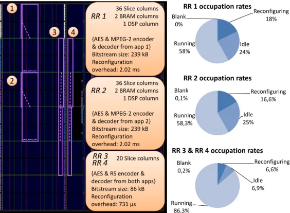
and four regions for two applications. Figure 7 shows the resulting floorplan and the possible task allocation for each reconfigurable region when running two applications in parallel, as well as occupation rates for each region. It also indicates uncompressed bitstream sizes in kB and the corresponding reconfiguration overhead when using FaRM in compression mode, with a compression ratio estimated to 26.7%.
The floorplan is composed of two types of reconfigurable regions: type 1 regions (RR 1 and RR 2) and type 2 regions (RR 3 and RR 4). Type 1 regions are the bigger regions, the only one capable of hosting an MPEG-2 encoder and decoder, while type 2 regions have been designed to fit an AES encoder and decoder as a result of the partitioning step. Occupation rates for each region are expressed as a percentage of the total simulation time. They are quite similar for regions of the same type: type 1 regions show a large reconfiguration time compared to pure execution time with a ratio of almost one to two, whereas type 2 regions spend most of the time executing tasks. This can be explained by the execution time, which is lower for MPEG-2 tasks compared to Reed-Solomon. Therefore, the regions hosting MPEG-2 can be released faster (going to idle state or being reconfigured) compared to regions hosting Reed-Solomon.
5.2. DSE for three applications in parallel
Another result from Table 3 is that partial reconfiguration is definitely of no use when running three applications in parallel. We could expect a constant improvement from the results of one and two applications, but PR
36 Slice columns 2 BRAM columns 1 DSP column {AES & MPEG-2 encoder & decoder from app 1} Bitstream size: 239 kB Reconfiguration overhead: 2.02 ms 1 2 3 4 36 Slice columns 2 BRAM columns 1 DSP column {AES & MPEG-2 encoder & decoder from app 2} Bitstream size: 239 kB Reconfiguration overhead: 2.02 ms
20 Slice columns {AES & RS encoder & decoder from both apps} Bitstream size: 86 kB Reconfiguration overhead: 731 µs Blank 0% Reconfiguring 18% Idle 24% Running 58% RR 1 occupation rates Blank 0,1% Reconfiguring 16,6% Idle 25% Running 58,3% RR 2 occupation rates Blank 0,2% Reconfiguring 6,6% Idle 6,9% Running 86,3%
RR 3 & RR 4 occupation rates
RR 1
RR 2
RR 3 RR 4
Figure 7: Floorplan for two applications in parallel
actually leads to a large resource overhead by using 9 reconfigurable regions. In fact, the issue comes from the reconfiguration mechanism of the FPGA. There is only one configuration port that can be active at a time on the FPGA, creating a bottleneck so that reconfigurations have to be sequenced using a first-come, first-served policy. In this case, a reconfiguration may not be done immediately, hence delaying task execution, resulting in the task missing its deadline. This phenomenon is highlighted by a huge configuration port occupation rate (almost 90% of the simulation time, while respectively 23 and 47 % for one and two applications). Therefore, in order to reduce it, the flow tends to increase the number of reconfigurable regions (up to nine RRs in our case).
Still, the solution provided by FoRTReSS for three applications executed in parallel shows poor results in terms of area compared to a static implemen-tation. However, it is possible to modify some of the architecture parameters in order to reduce this occupation rate and thus optimizing the PR solution.
For instance:
1. Higher Frequency: Reducing the reconfiguration time by running the configuration subsystem at a higher frequency. In [18], we succeeded in reaching a 200 MHz frequency for the configuration port and an AXI bus can be clocked at 150 MHz. In this case, as the limiting factor is clearly the bus access, the configuration port clock can be raised to 150 MHz. It is also possible to change the burst length (up to 256 beats in AXI specifications) [20].
2. Fewer reconfigurations: Reducing the number of reconfigurations by changing the algorithm execution granularity. Up until now, the worst case scenario was to reconfigure a RR after the task has processed one frame. By increasing this atomic number of frames with a factor n, we artificially reduce the total number of reconfigurations by n. This comes at the cost of an increased memory usage which is acceptable here since every frame is stored on an off-chip memory (e.g. 512 MB DDR3).
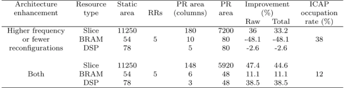
Table 4 shows the results obtained by using the solutions above with n = 2. Using one or the other solution results in the same floorplan with five reconfigurable regions, which is far better than the first solution obtained for three applications. However, there is still a huge wastage on memory blocks that can be avoided by combining both approaches. Unlike when using only one approach, the partitioning step succeeds and hence reduces the number of DSPs and memory needs, providing a better solution than a full static implementation. The configuration port occupation rate is also relatively low, which means that a better trade-off might be found by reducing frequencies. We do not develop this adjustment in the paper. Please note that it is also possible to use these approaches for one and two applications running. Nevertheless, the solution remains the same in terms of reconfigurable regions (and therefore area) but still lowers the memory cost for bitstream storage. However, this saving is not worth the cost of storing twice as many frames between tasks.
5.3. Final validation
In order to speed up the overall flow execution time, we decided to take an estimate of the bitstream compression ratio. Once the floorplan is infered by the tool, it is possible and recommended to validate the design with actual
Table 4: Area results for three applications in parallel on Virtex-6 LX240T
Architecture Resource Static PR area PR Improvement ICAP
enhancement type area RRs (columns) area (%) occupation
Raw Total rate (%)
Higher frequency Slice 11250 180 7200 36 33.2
or fewer BRAM 54 5 10 80 -48.1 -48.1 38
reconfigurations DSP 78 5 80 -2.6 -2.6
Slice 11250 148 5920 47.4 44.6
Both BRAM 54 5 6 48 11.1 11.1 12
DSP 78 3 48 38.5 38.5
compression ratios. Table 5 sums up these ratios, obtained by running Xilinx PlanAhead with a constraints file generated by FoRTReSS. The RRs are split into the previously defined types: type 1 and type 2. Aside from the application considered, these are the only two types of regions we obtained. Some ratios are not reported in the table, either because the RR cannot host the task (MPEG-2 encoder and decoder on RR type 2) or because such allocation is simply prohibited by the partitioning step (Reed-Solomon encoder and decoder on RR type 1).
Table 5: Actual bitstream compression ratios (in %)
Task RR type 1 RR type 2
MPEG-2 encoder 35.1 -MPEG-2 decoder 32.7 -AES encoder 45.3 13.1 AES decoder 49.2 7 Reed-Solomon encoder - 97.3 Reed-Solomon decoder - 94.1 Geometric mean 40 30.3
Compression ratios tend to be higher than expected, except for an AES encoder and decoder on RR type 2. However, the geometric mean for this RR type is very close to the estimate used. Therefore, the simulation launched with these values succeeds and the occupation rates stay close to what they were with compression estimation (see Fig. 7), with a variation of one or two
percent. This jitter on the aggregate reconfiguration time is reflected on the RR idle time, since the execution time is the same across simulations.
5.4. FoRTReSS execution times
Execution time can be split into two parts: RR determination (see Fig. 3) and DSE. RR determination is only done once at the beginning of the flow and depends on the number of tasks in the application. This time is tightly coupled to task complexity (whether they do or do not require different types of reconfigurable resources), target device (number of logic cells in the FPGA), and the shape allowed for reconfigurable regions that can be tuned by the designer. However, in our experience, this time does not exceed one second for each task. In the case of the Secure Box application, this first phase is completed within four seconds.
DSE includes the remaining steps of the FoRTReSS flow, including simu-lation. Thus, time spent on DSE varies a lot between use cases (5, 19 and 25 seconds respectively for one, two and three applications), due to an increasing number of SystemC simulations performed when raising the number of tasks in the application, each lasting up to a couple of seconds. This time is hard to estimate since it is impossible to know how many SystemC simulations will be performed during FoRTReSS iteration process (which is exactly the number of times the allocation is optimized).
These execution times do not include final verification done with the ac-tual bitstream compression rates. As mentioned earlier, compression rates are obtained by creating a PlanAhead project and effectively implementing the design and generating partial bitstreams. Each bitstream is generated within 10 to 15 minutes. This results in an important time overhead (nearly four hours for our two applications when targeting a Virtex-6 LX240T with Xilinx PlanAhead 13.3) but this step is necessary to fully validate the floor-plan when making use of bitstream compression. Measures have been done on a Core 2 Quad Q9650 processor running at 3 GHz with 8 GB of RAM, without taking advantage of multi-core parallelization.
6. Future works
Up until now, tasks are grouped on a reconfigurable region if and only if the RR resources are sufficient to host the tasks. We do not take care of possible differences between tasks interfaces, while interface uniformity is required to physically implement a task on a given region. In fact, we
assumed that every reconfigurable region provides an interface for each task that can be implemented. We are aware that this is clearly an important issue and it will be handled in the next versions of our flow. We want to add a task interface parameter into both task and RR representation that will be taken into account for grouping tasks sharing the same interface on one RR. At this point, FoRTReSS provides the designer with a set of reconfigurable regions and a scheduling scheme that ensure the application to meet its real-time constraints. However, the implementation step is not possible yet since there are several issues to take care of. For instance, tasks should have an interface to the reconfiguration manager in order to communicate its status. This could be done through a status register read via a slave bus access, but this is not specified yet. Another issue is the migration of the scheduling algorithm from the simulator to the MicroBlaze: we are currently working on a scheduler API common to both the simulator and the MicroBlaze to solve this issue.
7. Conclusion
In this paper, we presented FoRTResS, a flow to perform design space exploration on a partially reconfigurable design. Using information from synthesis tools, our flow automatically infers a possible architecture in terms of reconfigurable regions for a given application. The feasibility of this solu-tion is tested by a SystemC simulator that verifies if the applicasolu-tion real-time constraints are always met. A solution is evaluated by metrics such as ex-ternal fragmentation and total memory usage for configuration bitstream storage. We also discussed possible target architectures (FIFO-based or bus-based) compliant with our flow. We showed how it is possible to use the flow to solve some design issues in a small amount of time (30 seconds at most), especially when running three applications in parallel. We demon-strated the efficiency of our solutions that leads to saving up to 31.8% CLB resources, 11.1% BRAM resources and 38.5% DSP resources compared to a static implementation on a Xilinx Virtex-6 LX240T FPGA.
Acknowledgements
This work was carried out in the framework of project ARDMAHN [23] sponsored by the French National Research Agency, which aims at developing methodologies for home gateways integrating dynamic and partial reconfigu-ration.
References
[1] C. Kao, Benefits of Partial Reconfiguration, Xcell Journal 55 (2005) 65–67.
[2] K. Paulsson, M. H¨ubner, S. Bayar, J. Becker, Exploitation of Run-Time Partial Reconfiguration for Dynamic Power Management in Xilinx Spartan III-based Systems, in: International Conference on Field Pro-grammable Logic and Applications (FPL), 2008, pp. 699–700.
[3] S. Guccione, D. Levi, P. Sundararajan, JBits: A Java-based interface for reconfigurable computing, in: 2nd Annual Military and Aerospace Applications of Programmable Devices and Technologies Conference (MAPLD), Vol. 261, 1999.
[4] P. Manet, D. Maufroid, L. Tosi, G. Gailliard, O. Mulertt, M. Di Ciano, J.-D. Legat, D. Aulagnier, C. Gamrat, R. Liberati, V. La Barba, P. Cu-velier, B. Rousseau, P. Gelineau, An evaluation of dynamic partial re-configuration for signal and image processing in professional electronics applications, EURASIP J. Embedded Syst. 2008 (2008) 1:1–1:11. [5] K. Compton, S. Hauck, Reconfigurable computing: a survey of systems
and software, ACM Comput. Surv. 34 (2002) 171–210.
[6] R. Tessier, W. Burleson, Reconfigurable computing for digital signal processing: A survey, J. VLSI Signal Process. Syst. 28 (2001) 7–27. [7] Xilinx, Partial Reconfiguration User Guide (January 2012).
[8] A. A. Sohanghpurwala, P. Athanas, T. Frangieh, A. Wood, OpenPR: An Open-Source Partial-Reconfiguration Toolkit for Xilinx FPGAs, in: IPDPS Workshops, IEEE, 2011, pp. 228–235.
[9] Altera, Increasing Design Functionality with Partial and Dynamic Re-configuration in 28-nm FPGAs (July 2010).
[10] K. Bazargan, R. Kastner, M. Sarrafzadeh, 3-d floorplanning: Simulated annealing and greedy placement methods for reconfigurable computing systems, in: Proceedings of the Tenth IEEE International Workshop on Rapid System Prototyping (RSP), 1999.
[11] L. Singhal, E. Bozorgzadeh, Multi-layer floorplanning for reconfigurable designs, IET Computers & Digital Techniques 1 (4) (2007) 276–294. [12] A. Montone, M. D. Santambrogio, F. Redaelli, D. Sciuto,
Floorplace-ment for partial reconfigurable fpga-based systems, Int. J. Reconfig. Comput. 2011 (2011) 2:1–2:12.
[13] P. Banerjee, M. Sangtani, S. Sur-Kolay, Floorplanning for partial re-configuration in fpgas, in: Proceedings of the 2009 22nd International Conference on VLSI Design, VLSID ’09, IEEE Computer Society, Wash-ington, DC, USA, 2009, pp. 125–130.
[14] K. Vipin, S. A. Fahmy, Architecture-Aware Reconfiguration-Centric Floorplanning for Partial Reconfiguration, in: Proceedings of the 8th In-ternational Symposium on Applied Reconfigurable Computing (ARC), 2012, pp. 13–25.
[15] K. Vipin, S. A. Fahmy, Efficient region allocation for adaptive partial reconfiguration, in: International Conference on Field-Programmable Technology (FPT), 2011.
[16] N. Marques, H. Rabah, E.-N. Dabellani, Eric, S. Weber, Partially re-configurable entropy encoder for multi standards video adaptation, in: IEEE 15th International Symposium on Consumer Electronics (ISCE), Singapore, Singapore, 2011, pp. 492 – 496.
[17] F. Duhem, F. Muller, P. Lorenzini, Reconfiguration time overhead on field programmable gate arrays: reduction and cost model, IET Com-puters & Digital Techniques 6 (2) (2012) 105–113.
[18] F. Duhem, F. Muller, P. Lorenzini, FaRM: Fast Reconfiguration Man-ager for Reducing Reconfiguration Time Overhead on FPGA, in: Re-configurable Computing: Architectures, Tools and Applications, ARC ’11, 2011, pp. 253–260.
[19] F. Duhem, F. Muller, P. Lorenzini, Methodology for designing partially reconfigurable systems using transaction-level modeling, in: Conference on Design and Architectures for Signal and Image Processing (DASIP), 2011, pp. 316–322.
[21] Viotech, Viotech Home, http://www.viotech.net/. [22] OpenCores, OpenCores, http://opencores.org/.