DOCTORAT DE L'UNIVERSITÉ DE TOULOUSE
Délivré par :Institut National Polytechnique de Toulouse (Toulouse INP) Discipline ou spécialité :
Informatique et Télécommunication
Présentée et soutenue par :
M. FREDERIC GIROUDOT le vendredi 13 décembre 2019
Titre :
Unité de recherche : Ecole doctorale :
NoC-based Architectures for Real-Time Applications: Performance
Analysis and Design Space Exploration
Mathématiques, Informatique, Télécommunications de Toulouse (MITT)
Département Modèles pour l'Aérodynamique et l'Energétique (DMAE-ONERA) Directeur(s) de Thèse :
M. AHLEM MIFDAOUI M. EMMANUEL LOCHIN
Rapporteurs :
M. FRÉDÉRIC MALLET, INRIA SOPHIA ANTIPOLIS M. LAURENT GEORGE, UNIVERSITE MARNE LA VALLEE
Membre(s) du jury :
M. LAURENT GEORGE, ESIEE NOISY LE GRAND, Président M. AHLEM MIFDAOUI, ISAE-SUPAERO, Membre M. CLAIRE PAGETTI, ONERA TOULOUSE, Membre M. EMMANUEL LOCHIN, ISAE TOULOUSE, Membre
M. MARC GATTI, THALES AVIONICS, Membre
Monoprocessor architectures have reached their limits in regard to the computing power they offer vs the needs of modern systems. Although multicore architectures partially mitigate this limitation and are commonly used nowadays, they usually rely on intrinsi-cally non-scalable buses to interconnect the cores.
The manycore paradigm was introduced to tackle the scalability issue of bus-based architectures. It can scale up to hundreds of processing elements (PEs) on a single chip, by organizing them into computing tiles (holding one or several PEs). Intercore communication is usually done using a Network-on-Chip (NoC) that consists of interconnected on-chip routers on each tile.
However, manycore architectures raise numerous challenges, particularly for real-time applications. First, NoC-based communication tends to generate complex blocking patterns when congestion occurs, which complicates the analysis, since computing accurate worst-case delays becomes difficult. Second, running many applications on large Systems-on-Chip such as manycore architectures makes system design particularly crucial and complex. It complicates Design Space Exploration, as it multiplies the implementation alternatives that will guarantee the desired functionalities. Besides, given an architecture, mapping the tasks of all applications on the platform is a hard problem for which finding an optimal solution in a reasonable amount of time is not always possible.
Therefore, our first contributions address the need for computing tight worst-case delay bounds in wormhole NoCs. We first propose a buffer-aware worst-case timing analysis (BATA) to derive upper bounds on the worst-case end-to-end delays of constant-bit rate data flows transmitted over a NoC on a manycore architecture.
We then extend BATA to cover a wider range of traffic types, including bursty traffic flows, and heterogeneous architectures. The introduced method is called G-BATA for Graph-based BATA. In addition to covering a wider range of assumptions, G-BATA improves the computation time; thus increases the scalability of the method.
In a third part, we develop a method addressing design and mapping for applications with real-time constraints on manycore platforms. It combines model-based engineering tools (TTool) and simulation with our analytical verification technique (G-BATA) and tools (WoPANets) to provide an efficient design space exploration framework.
Finally, we validate our contributions on (a) a series of experiments on a physical plat-form and (b) a case study taken from the real world, the control application of an autonomous vehicle.
Les architectures mono-processeur montrent leurs limites en termes de puissance de calcul face aux besoins des systèmes actuels. Bien que les architectures multi-cœurs résolvent partiellement ce problème, elles utilisent en général des bus pour interconnecter les cœurs, et cette solution ne passe pas à l’échelle.
Les architectures dites pluri-cœurs ont été proposées pour palier les limitations des processeurs multi-cœurs. Elles peuvent réunir jusqu’à des centaines de cœurs sur une seule puce, organisés en dalles contenant une ou plusieurs entités de calcul. Elles sont gé-néralement munies d’un réseau sur puce permettant les échanges de données entre dalles.
Cependant, ces architectures posent de nombreux défis, en particulier pour les appli-cations temps-réel. D’une part, la communication via un réseau sur puce provoque des scénarios de blocage entre flux, ce qui complique l’analyse puisqu’il devient difficile de déterminer le pire cas. D’autre part, exécuter de nombreuses applications sur des systèmes sur puce de grande taille comme des architectures pluri-cœurs rend la conception de tels systèmes particulièrement complexe. Premièrement, cela multiplie les possibilités d’implémentation qui respectent les contraintes fonctionnelles, et l’ex-ploration d’architecture résultante est plus longue. Deuxièmement, déterminer de façon optimale la répartition des tâches à exécuter sur les entités de calcul n’est pas toujours possible en un temps raisonnable.
Ainsi, nos premières contributions s’intéressent à cette nécessité de pouvoir calculer des bornes fiables sur le pire cas des latence de transmission des flux de données emprun-tant des réseaux sur puce dits « wormhole ». Nous proposons un modèle analytique, BATA, prenant en compte la taille des mémoires tampon des routeurs et applicable à une configuration de flux de données périodiques générant un paquet à la fois.
Nous étendons ensuite le domaine d’applicabilité de BATA pour couvrir un modèle de traffic plus général ainsi que des architectures hétérogènes. Cette nouvelle méthode, appelée G-BATA, est basée sur une structure de graphe pour capturer les interférences possibles entre flux de données. Elle permet également de diminuer le temps de calcul de l’analyse, améliorant la scalabilité de l’approche.
Dans une troisième partie, nous proposons une méthode pour la conception de systèmes temps-réel basés sur des plateformes pluri-cœurs. Cette méthode intègre notre modèle d’analyse G-BATA dans un processus de conception systématique, faisant en outre in-tervenir un outil de modélisation et de simulation de systèmes reposant sur des concepts d’ingénierie dirigée par les modèles, TTool, et un logiciel pour l’analyse temps réel des réseaux, WoPANets.
Enfin, nous proposons une validation de nos contributions grâce à (a) une série d’expériences sur une plateforme physique et (b) une étude de cas d’application réelle, le système de contrôle d’un véhicule autonome.
A hero can be anyone.
—Bruce Wayne, The Dark Knight Rises To my supervisors, Ahlem and Emmanuel – I want to express my profound and genuine gratitude. I have never been a role model PhD student, so having role model supervisors was some kind of undeserved blessing. Many thanks for cheering me up in my worst days of discouragement, for believing in me and my work, for your immensely valuable input on papers and job applications, and most of all for letting me pursue my second passion.
To Guillaume, Stephen and Vincent, with whom I had the pleasure of working when I was in Sydney – thanks for making my experience at Data61 so amazing and valuable. I hope I see you again soon Down Under.
To Ludovic, who dragged me away from the vortex of my first contributions and opened to me the doors of TTool – I learnt so much working with you, and your efficiency at work was and continues to be an inspiration.
I would like to thank my thesis referees, Laurent George and Frédéric Mallet, for their feedback and the fresh look they provided on my work. Thanks, also, to my examinators, Claire Pagetti and Marc Gatti, for your input on my presentation and report.
Things would not have been the same without my work colleagues and friends, fellow PhD students and Doctors – I particularly want to mention:
Antoine, my equally-long-legged-sitting-in-front-of-me mate, mentor and famous WiFi expert, for joining me in the constant claim that 31000 is better than 31400; Eyal, fellow psytrance-listener, who left to another office too soon; Franco, the other bicycle-to-work-addict of my office; Ilia, for reminding me that no matter how much I struggle with red tape, there is always someone having it worse; Narjes, for her concerns about my (in)sanity and her inversely-proportional-to-her-size smile; Zoe, fellow adopted Aussie, for her knowledge about vermicomposting; Bastien, pilot, astrophysicist, TCP-specialist, seasoned artist in obnoxious puntastic jokes, for the always-appreciated observation nights that unveiled Saturn’s rings, Jupiter’s satellites, Mars and blinding views of the Moon; Doriane, Earth-explorer and sneaky raccoon who stole my NFC tag reader, for her shared love of electronic music and
for reminding me that there are no dumb questions; Henrick, inspirational alpha-vegetarian with a dash of perfectionism I sometimes wish I had, for what will go down in history as the “prank-that-went-too-far”; Lucas, for preventing my body from melting during the hottest days of summer, and whose will to experiment with blockchain rum was always appreciated; Clément, watercooling/lockpicking referent; John, whose PhD defence was even more impressive than his ability to ingest large amounts of junk food. Thanks for the shared laughs, meals, coffees, drinks, concerts, home parties, work hours; and for the many more things that helped me get through each day.
I also want to thank Christophe and Tanguy for trusting me with teaching part of their respective course in C and Java – it has been incredibly rewarding and I learnt a lot – as well as Odile, Alain, Rob and everyone at the DISC.
To Edo, Pauline, Eunbee and Lana – thanks for bearing your fair share of the living-under-the-same-roof-as-Fred pain. Your undiscontinued support makes you family to me now.
To my friends from prep class and engineering school – thanks for being part of the journey that brought me here. May you remain as brilliant as you are humble. To my friends in Toulouse, in Sydney and elsewhere, and to my family – a thousand of thank yous for your comforting presence and for not asking too much about how my PhD was going. I can’t name y’all but you know who you are.
To my aerial friends and acquaintances – I am so grateful for your support and for the breath of fresh air you have been when I was drowning under work. I still can’t believe I managed to get through this PhD while being able to train and compete. It was worth every struggle, injury, breakdown and freakout.
Thanks Maureen, Popo, Anne-Claire, Chacha, Olivia, Marion, Max, Cami, Dennis, Matt, Adam; and all the boys and girls I met around the world.
Special thanks to those who helped with the corrections of this manuscript: Alexandra, Ants, Béné, Charles, Lana, Taylor – you are the best.
I dedicate this thesis to my best friend Rhita, who, hopefully, will never have to go through the agony of reading it.
I Problem Statement and State of the Art 1
1 Introduction 3
2 Context and Problem Statement 7
2.1 Real-Time Systems Context . . . 8
2.1.1 Characteristics . . . 8
2.1.2 Examples . . . 8
2.1.3 Requirements and Challenges . . . 9
2.2 Manycore Platforms . . . 10
2.2.1 Topologies . . . 11
2.2.2 Forwarding Techniques and Flow Control . . . 15
2.2.3 Arbitration and Virtual Channels . . . 18
2.2.4 Routing Algorithms . . . 20
2.2.5 NoC Examples . . . 23
2.3 Discussion: NoCs and Real-Time Systems . . . 26
2.4 Conclusion . . . 29
3 State of the Art 31 3.1 Timing Analysis of NoCs . . . 32
3.1.1 Overview . . . 32
3.1.2 Scheduling Theory . . . 33
3.1.3 Compositional Performance Analysis . . . 36
3.1.4 Recursive Calculus . . . 37
3.1.5 Network Calculus . . . 38
3.1.6 Discussion . . . 40
3.2 System Design and Software/Hardware Mapping . . . 41
3.2.1 Design Space Exploration . . . 42
3.2.2 Task and Application Mapping on Manycore Architectures . 44 3.2.3 Discussion . . . 48
3.3 Conclusion . . . 48
II Contributions 51 4 BATA: Buffer-Aware Worst-Case Timing Analysis 53 4.1 Introduction . . . 54
4.2 Assumptions and System Model . . . 54
4.2.1 Network Model . . . 54
4.2.2 Flow Model . . . 57
4.3 Approach Overview . . . 57
4.3.2 Main Steps of BATA . . . 59
4.4 Indirect Blocking Analysis . . . 61
4.5 End-to-End Service Curve Computation . . . 65
4.5.1 Direct Blocking Latency . . . 65
4.5.2 Indirect Blocking Latency . . . 67
4.5.3 Computation Algorithm . . . 69 4.6 Illustrative Example . . . 70 4.7 Performance Evaluation . . . 73 4.7.1 Sensitivity Analysis . . . 74 4.7.2 Tightness Analysis . . . 77 4.7.3 Computational Analysis . . . 79 4.7.4 Comparative Study . . . 82 4.8 Conclusions . . . 84
5 G-BATA: Extending Buffer-Aware Timing Analysis 87 5.1 Problem Statement . . . 88
5.1.1 Illustrative Example . . . 88
5.1.2 Main Extensions . . . 90
5.2 Extended System Model . . . 91
5.2.1 Traffic Model . . . 91
5.2.2 Network Model . . . 91
5.3 Interference Graph Approach for Indirect Blocking Set . . . 93
5.4 Refining Indirect Blocking Latency . . . 96
5.5 G-BATA: Illustrative Example . . . 98
5.6 Performance Evaluation . . . 100
5.6.1 Computational Analysis . . . 101
5.6.2 Sensitivity Analysis . . . 107
5.6.3 Tightness Analysis . . . 112
5.7 Conclusions . . . 115
6 Hybrid Methodology for Design Space Exploration 117 6.1 Introduction . . . 117
6.2 Overview and Extended Workflow . . . 118
6.3 System Modeling: Adding a NoC Component in TTool . . . 119
6.3.1 Implementation . . . 119
6.3.2 Functional View . . . 120
6.3.3 Architecture . . . 124
6.4 Verification, NoC Generation and Simulation . . . 124
6.5 Performance Evaluation . . . 126
6.5.1 Example Modeling . . . 126
6.5.2 Analysis and Results . . . 128
7 Practical Applications 133
7.1 Experiments on TILE-Gx8036 . . . 134
7.1.1 Platform Characteristics . . . 134
7.1.2 Traffic Generation . . . 134
7.1.3 Latency Measurements . . . 136
7.1.4 Results and Discussion . . . 137
7.2 Control of an Autonomous Vehicle: Timing Analysis and Compara-tive Study . . . 138
7.3 Control of an Autonomous Vehicle: Modeling and DSE . . . 143
7.3.1 Functional Description . . . 144
7.3.2 Architecture Modeling . . . 145
7.3.3 Simulation . . . 145
7.4 Results and Conclusion . . . 146
III Conclusion 149 8 Conclusion 151 8.1 Summary of Contributions . . . 151
8.1.1 BATA . . . 151
8.1.2 G-BATA . . . 152
8.1.3 Hybrid Design Space Exploration . . . 152
8.1.4 Validation . . . 153
8.2 Perspectives . . . 153
8.2.1 Models and Approaches . . . 153
8.2.2 Tools . . . 155
IV Appendix 157 A Résumé en français 159 A.1 Introduction . . . 160
A.2 Contexte de la thèse . . . 162
A.2.1 Systèmes temps-réel . . . 162
A.2.2 Architectures pluri-cœurs . . . 163
A.3 État de l’art . . . 166
A.3.1 Analyse temps réel des réseaux sur puce . . . 166
A.3.2 Exploration d’architectures et mapping logiciel/matériel sur architectures pluri-cœurs . . . 170
A.4 Analyse temporelle pire cas des réseaux sur puce wormhole intégrant l’impact des mémoires tampon . . . 173
A.4.1 Modélisation du réseau et des flux . . . 173
A.4.2 Illustration du problème . . . 175
A.4.3 Formalisme et calculs . . . 176
A.4.4 Résumé de l’analyse de performance . . . 178
A.5 Analyse temps réel des NoCs wormhole hétérogènes par graphe
d’in-terférences . . . 182
A.5.1 Formalisme étendu . . . 182
A.5.2 Définition et construction du graphe d’interférence . . . 183
A.5.3 Analyse de performance . . . 185
A.5.4 Conclusion . . . 186
A.6 Approche hybride pour l’exploration d’architectures . . . 186
A.6.1 Workflow étendu . . . 187
A.6.2 Modélisation système du NoC . . . 187
A.6.3 Performance . . . 189
A.6.4 Conclusion . . . 191
A.7 Validation des contributions . . . 193
A.7.1 Analyse pire cas . . . 193
A.7.2 Modélisation sous TTool . . . 195
A.8 Conclusion . . . 196
A.8.1 Résumé des contributions . . . 196
A.8.2 Perspectives . . . 198
B Network Calculus Memo 201 B.1 Basics . . . 201
B.2 Notations . . . 203
C Case Study Data 207
D List of Publications 211
E List of Abbreviations 213
2.1 Ring network topology . . . 12
2.2 Mesh and Torus topologies . . . 13
2.3 Flattened Butterfly topology . . . 14
2.4 Bypass mechanism . . . 19
2.5 A typical deadlock scenario . . . 21
2.6 Intel SCC overview: grid and tile . . . 23
2.7 Tilera TILE-Gx8036 overview . . . 24
2.8 Kalray MPPA overview . . . 25
4.1 Typical 2D-mesh router . . . 55
4.2 Architecture of an input-buffered router and output multiplexing with arbitration modeling choices . . . 56
4.3 Example configuration and packet stalling . . . 58
4.4 Another configuration where flow 1 cannot be blocked by flow 3 . . . 59
4.5 Subpath illustration for the foi k . . . 62
4.6 Flow configuration on a 6×6 mesh NoC . . . 74
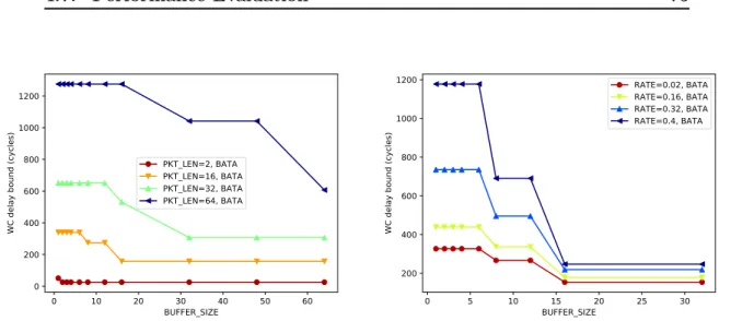
4.7 Buffer size impact on BATA end-to-end delay bounds . . . 75
4.8 Packet length impact on BATA end-to-end delay bounds . . . 75
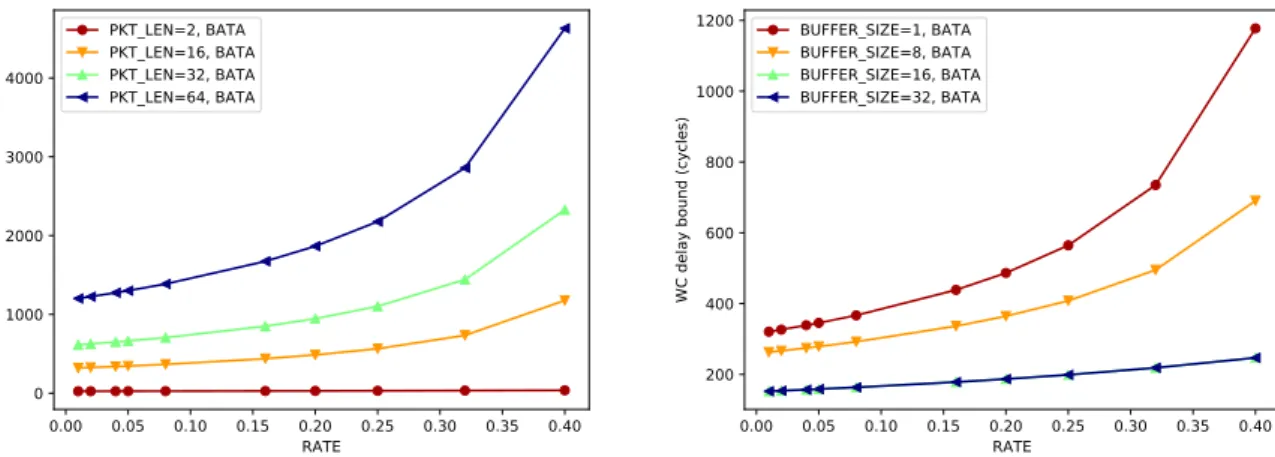
4.9 Rate impact on BATA end-to-end delay bounds . . . 76
4.10 Results of the BATA computational analysis . . . 80
4.11 Number of calls to the function endToEndServiceCurve() . . . 81
4.12 A simple configuration from [1]. . . 82
4.13 Predicted bounds for different values of bandwidth . . . 83
4.14 Delay bounds of flow 1 vs buffer size under CPA and NC approaches 83 5.1 Example configuration and subpaths computation with BATA . . . . 89
5.2 Packet configuration with two instances of flow 2 . . . 89
5.3 Main steps of G-BATA . . . 90
5.4 Subpaths computation with G-BATA approach . . . 100
5.5 Compared runtimes of BATA and G-BATA approaches . . . 101
5.6 Comparative study of the algorithmic complexity . . . 103
5.7 Scalability of G-BATA on large flow sets . . . 103
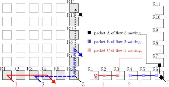
5.8 Quadrants of the NoC and illustration of flows from families A, B and C . . . 104
5.9 Runtimes vs flow number . . . 106
5.10 Studying the correlation between average DB index (resp. average IB index) and total runtime for 32-flow configurations . . . 107
5.11 Compared buffer size impact on end-to-end delay bounds . . . 108
5.12 Packet length impact on G-BATA end-to-end delay bounds . . . 110
5.13 Packet length impact on BATA end-to-end delay bounds . . . 110
5.15 Determining which approach should be used . . . 114
6.1 Workflow of the hybrid approach . . . 118
6.2 Extended workflow with implementation details . . . 120
6.3 NoC functional view . . . 121
6.4 Functional structure of a router . . . 121
6.5 Read and Write operations in the router model . . . 123
6.6 Control events in the router model . . . 123
6.7 Architectural view of the presented router (with task mapping) . . . 124
6.8 Example configuration . . . 126
6.9 Functional view of the example . . . 127
6.10 Activity diagrams . . . 127
6.11 Mapping example . . . 128
6.12 Distribution of end-to-end delays . . . 130
7.1 Main application algorithmic view . . . 135
7.2 TX and RX processes . . . 136
7.3 Experiment configurations 1 and 2 . . . 137
7.4 Experiment results for configuration 1 and 2 . . . 138
7.5 Worst-case end-to-end delay bounds comparative . . . 140
7.6 Delay bounds with 4, 2 and 1 VC with buffer size = 2 flits . . . 141
7.7 Task graph of the case study . . . 144
7.8 Activity diagram of control task 12 . . . 145
7.9 Architecture of the platform . . . 146
7.10 End-to-end delay measurements on the case study . . . 147
A.1 Topologies en grille et tore 2D . . . 164
A.2 Architecture d’un router de mesh 2D et niveaux d’arbitrage . . . 174
A.3 Exemple de blocage avec étalement des paquets . . . 175
A.4 Calcul d’un sous-chemin relativement au flux k . . . 177
A.5 Configuration test sur un réseau sur puce en grille 6×6 . . . 179
A.6 Résultats de l’analyse de scalabilité . . . 181
A.7 Processus de l’approche hybride . . . 187
A.8 Description fonctionnelle du réseau sur puce . . . 188
A.9 Description fonctionnelle d’un routeur 2 entrées, 2 sorties, 2 canaux virtuels . . . 189
A.10 Configuration considérée . . . 189
A.11 Vue fonctionnelle . . . 190
A.12 Diagrammes d’activité . . . 190
A.13 Architecture et mapping . . . 191
A.14 Distribution des délais mesurés . . . 192
A.15 Comparatif des bornes sur le délai de bout en bout . . . 194
A.16 Architecture de la plateforme . . . 196
2.1 Summary of main NoC topologies . . . 14
2.2 Forwarding techniques . . . 17
2.3 Flow control techniques . . . 18
2.4 Summary of design choices and their impact . . . 26
3.1 Summary of approaches for timing analysis of wormhole NoCs . . . 41
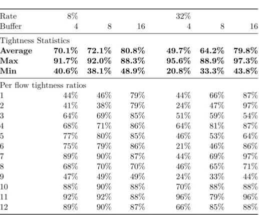
4.1 Tightness ratio results for the tested configuration . . . 78
5.1 Tightness Summary for both approaches, buffer size 4 flits and 16 flits113 6.1 Request times, injection times, ejection times and delays for all flows 129 7.1 Average tightness and tightness differences for various buffer sizes . . 139
7.2 Relative increase of the worst-case end-to-end delay bounds for B = 2 142 7.3 Runtimes of BATA and G-BATA for different NoC configurations . . 143
A.1 Résumé des choix de conception et leur impact . . . 166
A.2 Indices de finesse pour les configurations testées . . . 180
A.3 Résultats de simulation . . . 190
B.1 Summary of notations . . . 205
C.1 Original task-core mapping . . . 208
C.2 Flow set characteristics . . . 209
Anything that can go wrong, will go wrong.
—Murphy’s Law
Do you dance, Minnaloushe, do you dance?
—W.B. Yeats, The Cat and the Moon
Problem Statement and
State of the Art
Introduction
For a long time, processor architectures have been organized around a single pro-cessing element (PE). As performance requirements consistently increase, various optimizations and improvements have been made on such architectures. Adding specialized components and various controllers or coprocessors to handle repeti-tive tasks (such as network interfacing) or computationally expensive tasks (such as cryptographic functions) can unload the processing element, without fundamen-tally improving its performance.
Increasing the clock frequency is an option as well, but it comes at the price of a higher power consumption that causes more thermal dissipation. As such, it may not be appropriate for systems where only a passive cooling system is available, and is inherently limited by the physical resiliency of the chip.
Optimizing the processor pipeline, or using out-of-order execution and branch pre-diction techniques has also led to significant performance increase. However, it introduces undeterminism and additional design complexity. Moreover, attacks ex-ploiting out-of-order execution and/or speculative execution (Meltdown [2], Spectre [3]) have recently been implemented, which compromise memory isolation on many widely used processors. The immediate solutions to mitigate those vulnerabilities have a significant negative impact on performance [3].
Besides, none of the aforementioned techniques implements actual parallelism. Multiprocessor architectures have addressed this aspect. In addition to the various external devices or components, they classically feature several CPUs interconnected by a bus, but they are inherently limited in terms of scalability.
To cope with these limitations, the manycore paradigm was proposed [4]. It was made possible because chip technology has evolved to allow the integration of more and more transistors on the same silicon die. A manycore architecture is a set of “many”1 simple processors on a single chip, usually organized as an array of
1
tiles. To avoid bottleneck issues, each tile holds its local memory and cache, hence
cache coherency mechanisms and more generally memory requests must rely on an interconnect allowing inter-tile communication. Core-to-core message passing and access to external devices must be handled in a scalable way as well.
Several of such architectures are commercially available [5, 6, 7, 8].
In critical systems (e.g. avionics, aerospace and automotive), operating reliability is ensured through various costly certification processes. Therefore, there is still a strong trend to reuse components and architectures that are already certified; thus little incentive to migrate to a different architecture paradigm. Moreover, the multiplicity of processing elements and the concurrent execution of tasks make predictability of the system behavior harder to guarantee.
Nonetheless, the transition to manycore architecture seems unavoidable. Monopro-cessor architectures are likely to become scarcely available as their performance will be outranked by more recent manycore chips. Besides, monoprocessor architectures also struggle to meet the increasing computing power requirements in critical and mixed-criticality systems. The current paradigm in avionics is to multiply the number of monoprocessor computers, however such a solution decreases inherently the system scalability.
Therefore, ensuring predictable execution of critical applications on manycore plat-forms appears as one of the main challenges of the transition from monoprocessor to manycore architectures. There are several ways to contribute to this challenge. Mostly, they regard aspects of executing an application on a processing resource, with a particular focus on the specificities of manycore platforms compared to monoprocessor architectures (shared memory, shared communication media, and concurrent execution). In particular, these aspects include:
• enforcing task and memory isolation;
• mapping applications and tasks onto cores in a way that ensures tasks execute within their deadlines, while taking into account the dependencies between tasks;
• getting guarantees on communication delays between tasks;
• handling various levels of criticality among the applications running on the platform, and ensure least critical tasks do not impact the safe execution of most critical tasks;
This thesis will present our work on several specific aspects of real-time applica-tions execution on manycore chips, but try as much as possible to broaden the
applicability of our models to various platforms.
We start by giving the background we need for our work, and stating the problem we will be working on (Chapter 2). Then, we discuss the state-of-the art and the opportunities for possible contributions in Chapter 3. We then develop our contributions as follows:
• First, we address the intercore communication issue by introducing a timing analysis method applicable to a wide range of manycore architectures. Know-ing an upper bound on the traffic generated and/or consumed by each task running on a manycore platform, such an approach allows to derive worst-case performance bounds relative to the data flows.
• The result can be exploited to prove whether the communication require-ments are feasible with the given configuration and help orienting necessary alterations of the chosen architecture. In that respect, Chapter 4 presents a first approach, called BATA, for worst-case timing analysis of data flows on wormhole Networks-on-Chip, taking buffer size into account. We thoroughly evaluate BATA performances and find out that while it yields safe bounds with a tightness up to 80% on average for the tested configurations, the com-putation time needed grows rapidly with the number of flows, and it can only model constant-bit rate traffic.
• Second, in Chapter 5, we extend the first approach by introducing G-BATA, for “Graph-based BATA”. It simultaneously allows to model bursty traffic and heterogeneous architectures, and improves the computation time of the delay bounds. We evaluate its performances as well and compare them to the first model. We find out computations are up to 100 times faster than BATA for relatively small configurations, and the method is able to analyze large configurations (800 flows) with a reasonable analysis time (9 seconds per flow). G-BATA approach also provides bounds with a similar tightness compared to BATA.
• Third, we tackle task mapping and Design Space Exploration in Chapter 6. We integrate our intercore communication analysis approach into a system design methodology. Our proposal allows to model complex manycore-based systems and determine early in the design steps whether the real-time con-straints are met. To that end, we introduce additional models in the toolkit TTool [9] for design space exploration and implement our methodology using WoPANets [10, 11], a software for worst-case timing analysis of networks, to which we add a plugin supporting our timing analysis model.
• Fourth, in Chapter 7, we validate our contributions by confronting them to real-world applications. We perform experiments on a Tilera TILE-Gx8036 manycore chip to measure data flow end-to-end latencies and compare them to the bounds yielded by our model. We are able to prove that our approach is practically applicable to physical configurations and provides safe delay bounds on the configuration. We then apply our timing analysis and de-sign space exploration methodology to a case study of an autonomous vehicle control application.
• Finally, Chapter 8 concludes the thesis and unveils the future developments and perspectives of our work.
Pour cet écrit, j’ai dû aux sciences Offrir mon âme et trois années. Permets qu’il t’emmène, en apnée, Où les fils de ma pensée dansent.
* * *
Context and Problem
Statement
Contents
2.1 Real-Time Systems Context . . . . 8
2.1.1 Characteristics . . . 8 2.1.2 Examples . . . 8 2.1.3 Requirements and Challenges . . . 9
2.2 Manycore Platforms . . . . 10
2.2.1 Topologies . . . 11 2.2.2 Forwarding Techniques and Flow Control . . . 15 2.2.3 Arbitration and Virtual Channels . . . 18 2.2.4 Routing Algorithms . . . 20 2.2.5 NoC Examples . . . 23
2.3 Discussion: NoCs and Real-Time Systems . . . . 26
2.4 Conclusion . . . . 29
In this chapter, we narrow down the context of our work and we specify the prob-lem statement. We start by discussing the specificities of real-time systems in Section 2.1, and provide a few examples. We underline the main requirements and challenges raised by such systems. Then, we focus on manycore platforms and Networks-on-Chip, from an architectural and functional perspective, in Section 2.2. Afterwards, we discuss the relevance of the different paradigms in regard to real-time systems requirements and challenges in Section 2.3. Finally, based on the insight from the first sections, we conclude this chapter by a summary of the area we will explore in our research.
2.1
Real-Time Systems Context
2.1.1 Characteristics
A system is a real-time system when “the correctness of the system depends not only on the logical result of the computation but also on the time at which the results are produced” [12]. In other words, the result must be within a timing constraint (also called deadline) to be relevant. A computationally correct result that does not comply with the timing constraint may be useless, or dangerous.
Contrarily to non real-time systems (e.g. best effort systems), that seek to optimize average performance, real-time systems require first of all that all timing constraints are met, even in the worst-case execution scenario.
The impact of a deadline miss determines the criticality of the system or appli-cation, i.e. it quantifies how important it is that the system shall comply with its real-time constraints. If failure to meet the deadline leads to catastrophic consequences – death or huge material loss – the system is said to be hard real-time. If the deadline miss is of lesser importance and does not impact significantly the functionalities of the system, the system is said to be soft real-time. Finally, a system or part of a system that will be severely impacted by a deadline miss without catastrophic consequences is sometimes referred to as firm real-time.
Sometimes, complex systems are mixed-criticality systems. This means that they comprise several subsystems, applications or tasks that have different criticality levels. Analysis of such systems raises additional challenges, as the execution of a non-critical task should not impact the execution of a critical one.
2.1.2 Examples
In Aeronautics, Full Authority Digital Engine Controller (FADEC) [13] is an ap-plication in charge of controlling an aircraft jet engine. It receives information from sensors located in the engine, processes them, and, if need be, performs the appropriate action. Failure of this application to work properly may prevent an engine malfunction from being detected and mitigated. The possible consequences include the loss of an engine, damage to the aircraft and/or to the people on board. Therefore, FADEC is a hard real-time application.
(i) processing information from a stereo photogrammetric set of sensors; (ii) deriv-ing the absolute position of detected obstacles and addderiv-ing them to its database; (iii) adapting trajectory and monitoring vehicle stability. As these functions are critical to guarantee the integrity of the vehicle (and, whenever it is relevant, of the obstacles that may be humans), the system is hard real-time.
The video streaming service of Netflix is a real-time system, as failure to deliver the video frames in a timely manner could cause the movie being watched to freeze. However, a non-optimal streaming experience at home will not cause anything more serious than a few curse words being pronounced. It is certainly not critical. There-fore, such a system is soft real-time.
Australian Government’s Department of Home Affairs is a best-effort system for visa applications. For instance, 75% of applications for a subclass 407 training visa will be processed in 84 days or less, and 90% of applications will be processed in 4 months or less [15]. 1 There is no guarantee on the worst-case response time of the system.
2.1.3 Requirements and Challenges
Expected properties of real-time systems include in particular [16]:
1. Timeliness – results must not only be correct in terms of value, but also meet the associated deadline;
2. Design for peak load – the system must comply with its requirements even in the worst case scenario;
3. Predictability – to ensure that the performance requirements are met, the behavior of the system must be predictable;
4. Safety – we expect a valid behavior of the system in all circumstances. This includes fault tolerance and resilience to malicious attacks.
We consider safety issues as beyond the scope of this thesis, thus we choose to focus on the first three requirements.
Requirement 3 (predictability) is greatly impacted by design choices. For instance, common cache mechanisms improve the average execution time of a memory re-quest, but introduce undeterminism. When a cache miss occurs, the latency to perform the memory request can increase by several orders of magnitude. As we have to account for the worst case (Req. 2), it may be relevant to deactivate cache mechanisms to improve worst-case performance.
1
These informations are updated on a regular basis and may have evolved by the time this manuscript is read.
We will mostly rely on the predictability requirement to narrow down our study and leave out architecture paradigms and mechanisms that introduce undeterminism in the execution.
Additionally, real-time systems raise challenges that must be addressed, such as: 1. Scalability – with the increasing demands and foreseen size of real-time
systems in the short term, both the architecture paradigm and the related analysis methods must scale when considering large systems;
2. Complexity – to facilitate reconfiguration and decrease development and maintenance costs, designers favor simple architectures, from both a hard-ware and softhard-ware point of view. For instance, industrials in avionics and automotive tend to prefer using commercial off-the-shelf (COTS) technolo-gies to reduce costs.
Fulfilling real-time requirements should therefore not prevent these challenges to be taken into account.
Regardless, design choices will not be enough to ensure all real-time requirements are satisfied. Moreover, a trade-off must be found between addressing the afore-mentioned challenges while complying with the requirements of real-time systems. That is why there is a strong need for analytical models that are able to prove that the system complies with all requirements, particularly 1 and 2. In the fol-lowing sections, we will review design choices of manycore platforms and determine which of them are most suitable to help with real-time systems requirements and challenges.
2.2
Manycore Platforms
Manycore architectures need efficient intercore communication to make the most out of the additional computing power provided by the multiplicity of their processing elements. To avoid creating bottlenecks, they usually follow a NUMA (Non-Uniform Memory Access) paradigm, where each computing tile (holding one or several pro-cessing elements) has its local L1 cache and memory. Memory requests are thus addressed either locally or to a distant tile, and tiles are interconnected to allow not only distant memory requests, but also cache coherency mechanisms, core-to-core message passing and I/O and external devices access. Therefore, the choice of an interconnect is crucial from a performance point of view.
A simple interconnect such as a bus may be sufficient when there are only a few cores, but such a paradigm does not scale well over a few to a dozen of cores:
users competing for the use of the bus;
• the bus clocking frequency and synchronization are constrained by electrical properties of the chip technology.
Point-to-point wired communication, although solving the bandwidth issue, has a quadratic wiring complexity, thus does not scale well either. Essentially, an effi-cient interconnect will be a trade-off between hardware complexity and paradigm scalability, while guaranteeing communication predictability and timeliness. In that respect, Networks-on-Chip, proposed in [17, 18, 19], appear as a promis-ing solution for distributed, scalable interconnects. Networks-on-Chip, abbreviated NoC(s), follow a paradigm similar to classic switched networks – routers intercon-nected by links receive and forward data packets – but the on-chip nature of these networks carries specific constraints and characteristics, including mainly:
• the topology of the interconnection;
• the protocol(s) used to forward data from node to node and to handle con-gestion;
• the arbitration policy;
• the algorithm(s) used to compute packet routes; • the limited on-chip area;
• the place and route complexity and power consumption. • the hardware complexity;
• the amount of memory needed at each node; • the wiring complexity.
In the next sections, we will review the existing NoC architectures from these various points of view.
2.2.1 Topologies
It is generally not easy, or even impossible, to modify the hardware of an on-chip component. In that respect, and unless they are designed to be reconfigurable, NoCs topologies are static. To the best of our knowledge, there are no COTS architectures offering reconfigurable topologies, but it is something that could be imagined. Hereafter, we will only consider static topologies. The choice of the NoC topology impacts the scalability of the architecture (Challenge 1). To exhibit this impact, we consider a NoC N that we can assimilate to a directed, finite graph. We assume routers are vertices of the graph, denoted nodes(N ), while links are edges of the graph, denoted edges(N ). We present two metrics to characterize a NoC : network diameter and router radix. We will first need the following definition.
Definition 1. Minimal Path Length
Given any two routers R1, R2 in the network, the minimal path length from R1 to
R2 is the minimal number of “hops” or inter-router links that a packet must use
to go from R1 to R2. We denote it L(R1, R2). In graph terms, for any R1, R2 ∈
nodes(N ), L(R1, R2) is the shortest path from vertex R1 to vertex R2. Definition 2. Network Diameter
The network diameter DN is defined as:
DN = max
R1,R2∈nodes(N )
L(R1, R2)
In other words, network diameter is the maximum of all minimal path lengths over the network.
Definition 3. Router Radix
Considering only routers with the same number of inputs and outputs, the radix of router R is the number of input/output pairs of R. In graph terms, the router radix of R is the degree of vertex R.
With these notions, we now review several topologies described in the literature. The ring consists of N routers in a circular disposition. Each of them has 2 input/output pairs with its 2 closest neighbors (in a full duplex configuration) and an input/output pair with the local processing element (Figure 2.1). The radix of each router is constant and equals 3, but the diameter of this network topology is linear in the number of nodes (bN
2c in a full duplex configuration, N when the links to the neighbors are unidirectional). Moreover, the last point implies that the available bandwidth on a link can decrease rapidly with the number of flows.
A mesh consists of routers disposed at the intersections of a grid, most commonly a 2D grid ([20, 21, 22, 23, 24, 25]), although 3D meshes also have been thoroughly studied [26, 27], and higher dimension meshes are possible as well [20]. Routers are connected to the local tile and to their 2n neighbors (n being the dimension of the mesh), except for the border/corner routers (Figure 2.2). They have a constant radix, while the network diameter grows as O(√N) (provided the NoC is a square).
A torus is similar to a mesh, but the border routers are connected to the routers of the opposite border (Figure 2.2). The radix remains the same, and the network diameter has the same asymptotic complexity (up to a constant multiplier). Both these topologies exhibit a good scalability, mainly due to their acceptable router complexity. The main limiting factor is the diameter : for a 16 × 16 mesh NoC (256 nodes), the diameter is 31.
Figure 2.2 – Mesh and Torus topologies
Ring and n-dimensional torus are part of a larger family of topologies called the
k-ary n-cubes [20, 28]. A k-ary n-cube contains knnodes. For k > 2, each node has
2n neighbors (one in each dimension). For instance, a k-ary 1-cube is a ring with
k nodes, a k-ary 2-cube is a 2D torus with k2 nodes, a 3-ary 3-cube is a 3D torus
with 27 nodes.
In [29], the authors propose to adapt flattened butterfly topology to NoCs to prevent network diameter from increasing that fast with the number of nodes, and compare it to mesh topologies. The idea is that each router is connected to all routers on the same line and on the same column (Fig. 2.3, represented without the links to the tiles) and to one or more cores. If we connect each router to 4 cores, we are able to interconnect an 8 × 8-core chip using only 16 routers of maximum radix 10. The network diameter falls down to 2. Although this solution is not highly scalable, since following the same paradigm causes routers radix to explode rapidly
Topology Router radix Diameter Scalability
Ring constant = 3 O(N) Limited
n-dimensional mesh constant ≤ 2n + 1 O(√n
N) Good
n-dimensional torus constant = 2n + 1 O(√nN) Good
2D Flattened Butterfly O(√N) constant, 2 for a 2D grid Limited
Table 2.1 – Summary of main NoC topologies vs scalability issue
(O(p
(n))), solutions for connecting several 8 × 8 flattened butterfly topologies together are presented. However, they are not evaluated in detail and may suffer from a non-optimized application mapping since they lead to non-uniform NoC topologies.
Figure 2.3 – Flattened Butterfly topology
Finally, let us mention that for large platforms, it is possible to design a hierarchical interconnect. For instance, the Kalray MPPA Bostan [7, 30] has 256 processing cores and uses a 2D mesh NoC. The NoC is a 4 × 4 grid, connecting 16 tiles. Each tile holds 16 cores that are interconnected and share the local network interface to access the NoC. Hybrid interconnects combining a mesh and buses have been mentioned in [31] to improve performance, but the scalability issue has not been addressed for larger interconnects.
We summarized our quantitative insights of NoC topologies in Table 2.1. Network diameter is the limiting factor for the ring topology as it increases linearly with the
number of routers.
Flattened butterfly fixes this issue by ensuring a constant diameter, at the expense of the router radix. Router radix depends on the size of the network, therefore flattened butterfly is not suitable for direct use in a NoC topology.
Mesh and torus appear to be a good compromise. They allow for simple routers with a constant radix (similar to what a ring topology offers) while keeping the diameter reasonable as the number of router increases.
For larger platforms, hierarchical topologies can be explored. The most common approach is to group several (2 to 16) processing elements on each tile [8, 32, 7]. This allows to increase the number of interconnected processing elements without needing more routers, which means the diameter does not increase. This implies an increased utilization rate of the routers at the network interface, as several processing elements will use the same router to access the NoC. More complex hybrid interconnects have not been thoroughly evaluated.
2.2.2 Forwarding Techniques and Flow Control
Forwarding packets and managing data flows on the NoC can be done in many ways. The characteristics of the chosen techniques impact:
• the timeliness (Req. 1) and particularly the traffic latency;
• the platform complexity (Challenge 2) and specifically the needed on-chip memory;
• the predictability (Req. 3), regarding lossless transmission.
There are several ways to transmit packets over a network. The classical way of doing so is Store-and-Forward (S&F): at every hop, each packet is forwarded to the next network node. Once it reaches the next node, the routing decision is made and the packet can be forwarded to the next node, and so on until it reaches its destination. With this technique, it is necessary to:
• have enough memory at each router to hold at least the largest packet; • wait until each packet is completely stored to start forwarding it to the next
node.
This last point causes an additional latency on the transmission of a packet, that depends on the link bandwidth, packet length, and number of nodes to cross. For instance, if a packet of length L is transmitted over a path of N nodes connected by links of bandwidth C, the latency to transmit the packet over the network without congestion is L
Circuit switching [20, 33] addresses this issue. The idea of Circuit switching is that the sender of a packet uses a (smaller) control packet to request the needed resources along the path and establish a circuit before transmitting the packet from source to destination. The packet will then travel without experiencing congestion, and thus will not need to be buffered in any intermediate node. If the size of the control packet is Lc, the network latency is LCcN + CL. If Lc is small compared to
L, the length of the path has a minor impact on the network latency. However,
this mechanism requires to reserve the whole path of a packet to proceed to the transmission. This fact may be problematic on heavy-utilized networks, because it blocks all other packets from using even one part of the reserved path during the whole packet transmission.
Virtual Cut-Through (VCT), presented in [34], also reserves links on the path using a header, but without requiring to wait until a complete circuit is established. The packet is sent right away and will be entirely buffered in an intermediate node if contention occurs ahead. As with circuit switching, there is no need to wait for the whole packet at each node. However, the packet has to be entirely removed from the network if it is blocked at some point. If the header length is Lh, the network
latency without congestion is Lh
C N+
L
C, with a negligible impact of the path length
when Lh is small compared to L. VCT has the same buffer requirements as S&F,
since to cover worst-case congestion, it must be able to buffer an entire packet at each node.
Wormhole Routing proceeds with the same idea, by dividing a packet into flits of size Lf. The header progresses along the path, with the rest of the flits following
in a pipelined way. The main difference with VCT is that when the header is blocked, the packet does not have to be entirely buffered in the corresponding node. Instead, a flow control mechanism blocks the remaining flits where they are, and the transmission resumes when the header flit can move again. This drastically reduces the amount of memory needed at each node. The network latency without congestion has the same form as VCT and circuit switching: Lf
CN +
L C.
As far as memory use is concerned, wormhole routing has an advantage over other techniques as it requires only enough memory to store one flit at each router. It exhibits a low network latency when no congestion occurs, and the packet buffering in case of congestion can be tweaked by varying the available buffer size at each router. For instance, increasing the buffer size will allow to store a packet in fewer
Technique Packet Latency Per-node memory Path reservation S&F L CN ≥ L no circuit switching L C + Lc CN none yes VCT L C + Lh C N L no wormhole L C + Lf C N Lf no bufferless L C + Lf C N none no
Table 2.2 – Forwarding techniques and their requirements
nodes if it is blocked (or even more than one packet at each node), at the expense of memory requirements. For an on-chip system, carefully dimensioning memory will favorably impact power consumption and on-chip area.
Finally, we mention that bufferless techniques exist besides circuit switching, as described in [35, 36]. In [37], such a technique relies on a mechanism called
deflection routing (also referred to as hot-potato routing). The idea is similar
to wormhole routing, except that flits are never buffered. If the requested output is not available, flits are routed to a different one and never remain in a router. Such a technique is intrinsically limited to unicast transmission, be-cause at each router, there has to be at most as many exiting flits than entering flits.
We synthesized the characteristics of forwarding techniques in Table 2.2, in terms of packet latency, buffer memory needs and path reservation.
To handle packets when congestion occurs, forwarding techniques rely on a mech-anism called flow control (see [33]). We can mainly distinct 3 types of flow control mechanisms:
Delay-based or Credit-based: when a packet requests a resource that is unavail-able, it is buffered and waits until it is granted the use of the resource. Delay-based flow control can be implemented using a system of credits issued from each input that grant the upstream output the ability to forward one flit. Such a mechanism enables lossless transmissions and can be used with most of the forwarding tech-niques mentioned earlier (S&F, VCT, wormhole). This mechanism induces a higher end-to-end delay when there is congestion to guarantee lossless transmission. Loss-based: when a packet requests a resource that is unavailable, it is dropped after a certain time and has to be retransmitted. The retransmission is usually managed by a higher layer. Such a mechanism can be used with S&F, VCT and
Flow control Predictability Delay-based good
Loss-based limited Deflection-based limited
Table 2.3 – Flow control techniques and their predictability
wormhole routing as well. It may help reduce congestion in the network during periods of heavy utilization and improve the average latency, but introduces un-determinism due to the drop and retransmission issues. In particular, it is hard to bound the worst-case latency of a packet, considering it may be dropped an arbitrary number of times due to congestion.
Deflection-based: when a packet requests a resource that is unavailable, it is deflected from its original route. This mechanism also allows lossless transmission and improves load-balancing, because of its ability to reroute packets towards non-utilized links. Similarly to loss-based flow control, it comes at the price of an additional unpredictability regarding the delay experienced by a packet, because it is difficult to bound the number of times a packet may be deflected from its original path to destination.
We recap these characteristics in Table 2.3.
2.2.3 Arbitration and Virtual Channels
When several packets are competing for the use of one resource, the router has to decide which of them will be granted the use of the resource. The arbitration levels in the router may vary depending on the router architecture, but the underlying policies to favor one packet over another are generally among the following: First-Come First-Served (FCFS):flits arriving at a router are served according to the time they arrived at the router, in a First-In First-Out way. This is the simplest policy.
Round-Robin (RR): at each router, all entities requesting the use of a resource are each allocated a certain amount of credit. Each of them is served until its credit runs out. Then, the arbiter serves the next entity, and so on. Each entity recovers its full credit amount when the arbiter switches to the next entity.
Weighted Round-Robin (WRR): WRR is the same as RR, except that the amount of credit assigned to the various entities may differ and favor some entities over others. The weight of an entity is the ratio of its amount of credit to the total amount of credit. This way, the sum of all weights equals 1. WRR and RR exhibit
one flit of packet 1 can move
buffer is now full, packet 1 is blocked
packet 2 can move while 1 is blocked
1
2
Figure 2.4 – Bypass mechanism
a good predictability (Req. 3) in terms of granted service.
Fixed Priority (FP): this policy requires packets to have a priority attribute. In case of concurrent request for the same resource, a packet with a higher priority will be served before a packet of a lower priority. This impacts the predictability. For higher priority packets, it increases predictability, as they are guaranteed a certain service. As such, it also improves timeliness (Req. 1) for higher priority levels. For lower priority packets, it decreases predictability, as their granted service depends a lot on the presence of higher priority packets competing for the same resources.
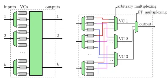
Virtual Channels (VCs), introduced in [38], are a way to share one physical link into separate logical channels, by implementing separate buffer queues at each router [39]. Packets in different VCs will use the same links from node to node but they will queue in different buffers. This especially allows one packet to bypass another that is blocked instead of having to queue behind it. On Figure 2.4, we present an example of a bypass scenario enabled by VCs. Initially, packet 1 is using the link and forwarding one flit to the next buffer, while packet 2 has to wait because the link is being used by packet 1. The next buffer on the path of packet 1 is then full, so packet 1 cannot move further. However, packet 2 is using another VC, and the next buffer of this VC is not full. Therefore, packet 2 can resume its transmission. Such a mechanism improves overall link utilization while reducing congestion. It may help with system scalability (Challenge 1), but at the expense of an increased complexity (Challenge 2).
Typically, VCs are used to provide different guarantees to different traffic classes, but they can also be used for preventing deadlocks (packets being forever blocked in the network, see Section 2.2.4), by breaking cyclic dependencies between the
resources requested by packets [40]. Packets may be statically assigned to one VC, or change VC during their transmission, depending on what VCs are used for. A typical use of VCs is to implement a FP arbitration policy. To do that, one can map one priority level to a VC (this is done in [41]), or several priority levels to one VC. Another way, mentioned in [42], is to do a local mapping of priority levels to VCs at each node, depending on the flow communication pattern. Provided there are enough VCs, this can ensure only one flow is mapped to each VC at each router and/or minimize the number of needed VCs. This requires to know the path of the flows, and do an offline static mapping of priority levels on VCs.
Note that in routers, depending on the architecture, there may be several arbi-tration levels. For instance, one can arbitrate between packets depending on the input they come from or on the VC they use, with a different arbitration policy.
Arbitration policies that favor predictability are mostly (weighted) round-robin and fixed priority. FCFS, although simpler, provides a service that depends a lot on how many packets request the same resource, and at what time they do. RR is relatively simple to implement and provides the best fairness to all traffic classes. Fixed priority requires to handle priority attributes that can either be read from each packet, or determined using virtual channels, and in that way may increase hardware and/or software complexity. It is less fair than RR and degrades the predictability of the service granted to lower priority classes, but this may be a possibility worth exploring when dealing with mixed criticality traffic or flows with different timing requirements (real-time and best-effort).
2.2.4 Routing Algorithms
Knowing the flow control mechanism and forwarding technique used to transmit a packet from node to node is not enough to successfully transmit a packet over the NoC. In order for a packet to reach its destination, each node should know where a flit is supposed to be forwarded. This is ensured by choosing an appropriate way of determining the path of a packet from source to destination. Such a principle is called a routing algorithm. In this section, we will review different algorithms.
A routing algorithm, along with the chosen flow control mechanism, must ensure that all packets reach their destinations, and as such it should prevent two phenom-ena: deadlock and livelock. The former occurs when a packet or a flit is waiting to be granted the use of a resource used by another flit or packet, that is in turn
waiting for a resource to be freed, and so on so forth, with ultimately a packet or flit waiting for the resource used by the packet or flit of interest to become avail-able. It occurs when resource requests dependencies form a cycle. Such a scenario is represented on Figure 2.5.
Figure 2.5 – A typical deadlock scenario
Here, each head flit of the purple, green, blue and red packet respectively is waiting for a resource used by a flit of green, blue, red and purple packet, respectively. The situation cannot evolve and the packets are blocked forever. A livelock occurs when a packet progresses in the network without ever reaching its destination. Typically, such a scenario is imaginable with bufferless techniques (a packet is never blocked) if the packet keeps being deflected from its destination due to an unfair arbitration policy with packets of contending flows.
Hence, the choice of a routing algorithm will impact the predictability requirement (Req. 3). We can distinct several characteristics of routing algorithms, as detailed in [33].
Central vs distributed: central routing relies on one common entity to compute the routes for all packets. Distributed routing has multiple entities capable of deciding all or part of the route a packet will use. Central routing can be done either offline for configurations where all data flows are known, or online when meaning the computing entity receives a request for each packet to be sent. The latter option does not scale well because it creates a bottleneck at the computing entity (Challenge 1). The former option allows to balance link utilization, but implies that all data flows must be known in advance. Distributed routing can also be done offline e.g. with the used of routing tables at each node, or dynamically.
It shows better scalability than centralized routing.
Source routing vs hop routing: both can be classified as subfamilies of dis-tributed routing algorithms. Algorithms based on source routing compute the whole path of a packet before it is sent. Algorithms based on hop routing rely on each node to make the decision for the next hop. Choosing one or the other may slightly impact complexity, but the way it does depends on other factors.
Deterministic vs adaptive: Given a source SRC and a destination DST, a de-terministic routing algorithm will always give the same route from SRC to DST. Running an adaptive algorithm twice with the same SRC and DST may, however, output different routes depending on the circumstances. It can adapt the path to live or unpredictable events, e.g. congestion or link failure. Adaptive routing can help mitigate congestion at the expense of predictability. In that respect, determin-istic routing will fit better for real-time systems (Req. 3).
Minimal vs nonminimal: the path computed can be either (one of) the shortest paths available, or not. It is interesting to notice that in the general case of a
k-ary n-cube, a deterministic, deadlock-free, minimal routing algorithm does not
exist, but nonminimal routing algorithms have been introduced for such topologies [40, 20].
Routing algorithm possibilities are partly conditioned by the topology. For mesh and torus of an arbitrary dimension, the dimension-ordered routing (DOR) is a typical example of a deterministic, distributed and deadlock-free algorithm. We choose an order on the n dimensions of the topology, from 1 to n. Knowing the position of the current node, (x1, · · · , xn), and the position of the destination node,
(x0
1, · · · , x0n), the packet is first routed along the dimension 1 until x1 = x01. Then, it is routed along dimension 2, and so on, until finally xn= x0n. For a 2D mesh (or
torus), the two possible DOR are X first and Y first, depending on which dimension is picked first.
Deflection routing, used especially in bufferless architectures, can be based on a preferred route, e.g. computed using a minimal routing algorithm. In the case two packets compete for the same output, the arbiter will deflect one of them from its preferred route. To avoid a packet being unfairly or endlessly deflected (which could cause a livelock), dedicated arbitration mechanisms have been developed when deflection is necessary [37].
Finally, the turn model, introduced in [43], allows to design partially adaptive or deterministic routing algorithms for n-dimensional meshes and k-ary n-cubes.
2.2.5 NoC Examples
2.2.5.1 Intel SCC
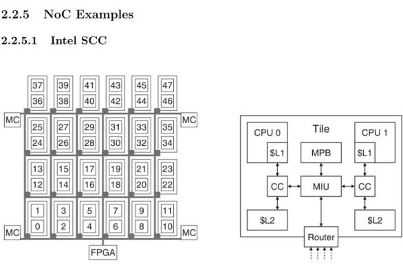
Figure 2.6 – Intel SCC overview: grid (left) and tile (right)
Intel’s Single-chip Cloud Computer is a manycore chip developed for research pur-poses [44, 8]. It features 24 2-core tiles interconnected via a 4×6 mesh NoC. Routing policy is XY. Apart from the tiles, the SCC contains four memory controllers (MC) and an FPGA.
An overview of the SCC architecture is shown on Figure 2.6. On each tile, the two cores have their own L1 cache for data and instructions, and a L2 data cache with the associated cache controller (CC). A mesh interface unit (MIU) allows cores to access the NoC and handles the buffer that stores incoming packets, the message passing buffer (MPB).
Intel SCC has been widely used for research purposes, including in real-time-oriented papers [45, 46].
2.2.5.2 Tilera TILE-Gx8036 and TILE-Gx Series
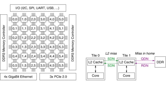
The TILE-Gx8036 [5] is a 36-core chip with a 2D-mesh NoC. The NoC is constituted of several independent networks for various types of traffic, but the user mostly has control over one of them, called UDN (User Dynamic Network). Among the other subnetworks, the I/O Dynamic Network (IDN) handles I/O devices access, while the memory system uses the QDN (reQuest Dynamic Network), RDN (Response
Figure 2.7 – Tilera TILE-Gx8036 overview: NoC and devices (left) and memory requests handling (right)
Dynamic Network) and the SDN (memory snoop network) to handle various oper-ations. The UDN has no virtual channels and supports dimension-ordered routing (either X-first or Y-first). Buffers are located at the input of routers and can hold 3 flits. The technological latency of the routers is one cycle.
The arbitration mechanism of routers is central. Therefore, if two flits cross the router using different inputs and requesting different outputs, one of them will experience an additional delay of one cycle, as the arbitration mechanism will handle them one after the other. A far as arbitration mechanisms between input ports are concerned, the chip offers a classic Round-Robin policy and a Network Priority policy. The latter favors traffic that is already on the NoC over traffic requesting a local input port (injection).
Note that similar chips with more cores are also available, such as Mellanox TILE-Gx72 [6]. An overview of the TILE-Gx with 36 cores is shown on Figure 2.7.
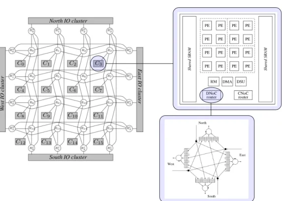
2.2.5.3 Kalray MPPA series
Kalray MPPA-256 [7] is a 256-core chip. It is organized in 16 tiles connected by two 4 × 4 2D-torus NoC. One, the Data-NoC, is dedicated to data transfers, the other handles small control messages (Control-NoC). Buffers are located at the outputs routers, and there are 4 of these buffers at each output (one for each of the 4 other interfaces). The arbitration between contending flows is round-robin, and unlike the TILE-Gx, flows crossing a router without interface conflict do not delay each
Figure 2.8 – Kalray MPPA overview: NoC (top left), tile (top right) and router (bottom)
other.
Both NoCs support source routing. All turns a packet must take to reach its destination are written by software in the header before the packet is sent. Flow control relies on traffic shapers, that can throttle the injection rate of flows in the NoC and subsequently ensure that buffers are never full (thus no backpressure happens).
NoCs also handle multicast (deliver the packet to some of the nodes on its route) and broadcast (deliver the packet to all nodes on its route). Note that these definitions of multicast and broadcast differ from what is usually assumed in classical networks. Each tile contains 16 general purpose cores, an additional core to manage resources of the local tile (resource manager or RM), a DMA device to send data over the NoC, and memory.
We present the architecture of the Kalray MPPA on Figure 2.8. We also included the architecture of a router, as it is significantly different from many other manycore NoC routers.
Predictability Scalability Complexity Restriction
Topology mesh and torus
Forwarding wormhole
Flow control delay-based
Arbitration RR, WRR, FP
VCs implementing FP
Routing deterministic,
dis-tributed Table 2.4 – Summary of design choices and their impact
2.3
Discussion: NoCs and Real-Time Systems
In this section, we first summarize our study of NoCs architectures and design choices and their impact on real-time requirements and challenges. Then, with the insight of existing architectures, we explain what our focus will be in the next sections. We tackle the predictability requirement by considering paradigms that favor deterministic behavior, so that bounding the worst-case is possible (Req. 3). Similarly, we discard paradigms that would prevent the system to scale (Challenge 1). Finally, we favor solutions that decrease memory requirements and on-chip complexity (Challenge 2).
Table 2.4 recaps the various design choices in NoCs for manycore architectures. We highlight the main impacts they have on requirements and challenges by putting a check mark in the appropriate cell, and use this insight to determine whether we restrict the focus of our work to specific paradigms. These restrictions are shown in the last column. No check mark in a column does not mean the considered design paradigm has no impact on the corresponding requirement, but rather that its impact is limited or considered not crucial, and therefore will not restrict the focus of our work.
From a predictability point of view, we want to avoid techniques that do not provide worst-case guarantees. In terms of topologies, there is no predictability-related incentive to pick one topology over another. The relevant criteria to favor one paradigm over another have to do with scalability and on-chip place-and-route complexity. Commercially available chips remain generally based on 2D-mesh and torus, and occasionally 3D-mesh. They keep the on-chip wiring simple, are adapted to routing algorithms that are simple to implement, and they scale well, especially