Developing approximation architectures for decision-making in real-time systems

Developing Approximation Architectures for

Decision-Making in Real-Time Systems

by

Lee Ling

Submitted to the Department of Mechanical Engineering

in partial fulfillment of the requirements for the degree of

Bachelor of Science in Engineering as Recommended

by the Department of Mechanical Engineering

at the

MASSACHUSETTS INSTITUTE OF TECHNOLOGY

June 2006

) Lee Ling, MMVI. All rights reserved.

The author hereby grants to MIT permission to reproduce and

distribute publicly paper and electronic copies of this thesis document

in whole or in part.

Author

...

Department of Mechanical Engineering

May 12, 2006

Certified by ...

_ _...

-..-

. .

Daniela P. de Farias

Assast.Professor

of Mechanical Engineering

Thesis Supervisor

Accepted by ...

John H. Lienhard V

P rofessor of Mechanical Engineering

Chairman, Undergraduate Thesis Committee

ARCHIVES MASSACHUSETTS INSTITUTE OF TECHNOLOGY

[..,I

AUG 0 2 2006 w -

-Developing Approximation Architectures for

Decision-Making in Real-Time Systems

by

Lee Ling

Submitted to the Department of Mechanical Engineering

on May 12, 2006, in partial fulfillment of the requirements for the degree of

Bachelor of Science in Engineering as Recommended by the Department of Mechanical Engineering

Abstract

This thesis studies the design of basis functions in approximate linear programming (ALP) as a decision-making tool. A case study on a robotic control problem shows that feature-based basis functions are very effective because they are able to

cap-ture the characteristics and cost struccap-ture of the problem. State-space partitioning,

polynomials and other non-linear combinations of state parameters are also used in the ALP. However, design of these basis functions requires more trial-and-error. Simulation results show that control policy generated by the approximate linear

pro-gramming algorithm matches and sometimes surpasses that of heuristics. Moreover,

optimal policies are found well before value function estimates reach optimality. The

ALP scales well with problem size and the number of basis functions required to find the optimal policy does not increase significantly in larger scale systems. The promis-ing results shed light on the possibility of applypromis-ing approximate linear programmpromis-ing

to other large-scale problems that are computationally intractable using traditional

dynamic programming methods.

Thesis Supervisor: Daniela P. de Farias

Acknowledgments

Here I would like to thank my thesis supervisor Prof. Daniela de Farias for her invaluable guidance and encouragement throughout the year. The research will not be the same without her insight and suggestions. I must also thank Mario Valenti for his immense support. My education at MIT is deeply enriched by this research experience and close collaboration with Prof. de Farias and Mario. Finally, I would like to thank my academic advisor Prof. Derek Rowell for all his support during my undergraduate years. He has greatly influenced me by his strong ethical values and unending interests in academic pursuits.

Contents

1 Introduction

1.1 Motivation for Approximate Linear

Programming.

1.2 Application - A Robotic Control Problem ...

2 The Model

2.1 The Basic Problem ...

2.2 The Approximate Linear Programming Approach 2.3 Robotic Control as a Markov Decision Process . .

2.3.1 State Space. 2.3.2 Action Space.

2.3.3 Local Cost at Each State ...

2.3.4 Probability Transition Function ...

3 Methodology

3.1 The Approximate Linear Programming Approach

3.2 Approximation Architecture.

3.2.1 State Space Partitioning . . . .

3.2.2 Features Mapping . 3.2.3 Polynomials ...

3.2.4 Others ...

4 Results and Discussion

11 12 13 15 15 16 17 17 18 18 19 21 21 22 22 23 23 24 25

...

...

...

...

...

...

...

...

...

...

...

...

...

4.1 Scope of the experiments ... . 25

4.2 Heuristics ... 26

4.3 Summary of Results ... 26

4.3.1 Analysis of Object Value Plots ... 27

4.3.2 Analysis of Value Function Estimation ... 27

4.3.3 Overall Performance of ALP Algorithm ... 28

4.4 Limitations and Improvements ... 28

5 Conclusion

31

List of Figures

Value and Value Value Value Value Value Value

and

and

and

and

and

Value Value Value Value Value

Function

Function

Function

Function

Function

Function

Estimate with

Estimate with

Estimate with

Estimate with

Estimate with

Estimate with

801 states .

2058 states .

2171 states .

4341 states .

11009 states 19741 states A-1 A-2 A-3 A-4 A-5 A-6 Objective Objective Objective Objective Objective Objective . . 33 . . 34 .. 35 . . 36 . . 37 . . 38

Chapter 1

Introduction

Sequential decision-making in large-scale systems is a challenge faced by many busi-nesses. For example, in a complex job shop environment where raw materials must be processed in a timely fashion, common decisions related to the scheduling of main-tenance, manpower and machine usage can have a large effect on the future profit margin of the company. To minimize losses it is important to solve these problems in a timely fashion, whereby decisions are made based on the current state of the system. However, it is difficult to find 'optimal' solutions for these problems even with modern computational capabilities. As a result, many techniques have been developed to find solutions to large-scale decision-making problems. For example, dynamic programming methods have been used to find solutions to these problems. In order to use dynamic programming techniques, one must first define an underly-ing dynamic system and a local cost function that is additive over time. Generally speaking, this dynamic system must have a state space, an action space, and a state

transition function defining the evolution of the states over time. In addition, the

local cost function is defined for each state-action pair. In general, the goal of this technique is to find a control law or policy which maps every state to a specific action

and minimizes the total future cost (the 'cost-to-go') over a particular time horizon.

The goal of this research project is to develop an efficient computational architecture

for dynamic programming problems by adopting the approximate linear programming

1.1 Motivation for Approximate Linear

Programming

Although dynamic programming is a very useful and powerful technique for finding optimal solutions to sequential decision-making problems under uncertainty, it does not scale well with the size of the problem. Dynamic programming relies on the

computation of the exact cost-to-go at every state in order to map the state to an

optimal action. However, the computational power required to calculate and store the cost function grows exponentially with the number of state variables in the system. One would soon realize that seemingly simple problems become unmanageable very quickly. As a result, large-scale problems cannot be easily solved in real-time using

this technique, and this limitation is called The Curse of Dimensionality.

There-fore, approximation structures have been developed to reduce computation time. For example, the cost-to-go function may be approximated by a linear combination of known functions of the state. This reduces the dimension of the original problem to the number of known functions used. The problem therefore reduces to finding the best set of weights to approximate the cost-to-go function.

The objective of this research project is to develop approximation architectures

for decision-making in real-time systems using approximate dynamic programming. Building upon the idea of traditional linear regression, an algorithm for picking ap-propriate basis functions and their weights will be developed to approximate the cost-to-go function of the system. The estimated value function will then be used to generate a policy that maps the optimal action to each possible state. The perfor-mance of the policy generated will be compared to that of exact solutions in small scale problems, and to performance of heuristics in large-scale problems, in which exact solutions are very difficult to find, if possible at all.

1.2 Application - A Robotic Control Problem

Intuitively, approximation architecture works the best if it is developed based on the

characteristics of the system being modeled. In this project, the techniques of picking

basis functions and their performance is illustrated by a robotic control application.

Imagine there is an ambitious robot on Mars which manufactures bits and pieces of itself every day, assembles the parts, tries to make many copies of itself and hoping

that it can eventually take over the planet. The robot has a home base that is N

steps away from the construction station. The robot gets recharged, repaired as well

as deliver the finished products at the base. In the work station, the robot must

work consecutively for T time steps on a product unless it runs out of energy. At

each time step, the robot can decide whether it wants to return to the base (1 step

backwards), move towards the work station (1 step forward), or remain stationary.

The displacement happens with probability 1.

The robot, though ambitious, is subject to the following constraints and

mainte-nance costs:

* The construction device on the robot is fragile and breaks with probability p at

any time. If it breaks, the robot will need to go back to the base for maintenance.

* The robot only has F time steps worth of energy, where F > 2 * N + T.

* There is a high maintenance cost of

M

1 units with re-charging included.

* At any point in time, if the robot runs out of energy, it will need to be taken

back to the base to be recharged, which will incur a high cost of M2 units.

* Normal operating cost of the robot is 1 unit per time step.

Several questions are raised: What is the optimal policy at each state? How is the policy computed? For different values of p, how does this policy change? In order to answer those questions, the robotic control problem will be modeled as a Markov Decision Process. Understanding the cost structure of the problem will help us find

of this problem will also provide insights on how to pick the set of basis functions and their weights to approximate the cost functions of larger-scale control problems. Moreover, additional basis functions can be obtained by state space partitioning. Detailed descriptions of the techniques and the basis functions used in this problem will be discussed in the methodology section.

Chapter 2

The Model

In this project, a real-time system will be modeled as a Markov decision process characterized by a tuple

{S,

A., P.(-, .), g.(.)} - a state space, an action space, a state

transition probability function and a cost function associated with each state-action pair. [3] The scope of this project is a discrete-time dynamic system in infinite horizon, which is defined below as the 'basic' problem we are trying to solve [3]:

2.1 The Basic Problem

Given a Markov Decision Process, with state space S, action space A, transition probability Pa(x,y), cost function ga(x), we want to find a policy (or control law)

u: S

-+

A to solve the following optimization problem:

We consider infinite-horizon discounted-cost problems with a discount factor a E [0, 1] so that our problem is equivalent to solving

00

min E[y atg,(,,)(xt)Ixo

=

x]

U(.,.) t=O

For each policy u, the cost-to-go at state x is given by: 00

Ju(x) = E[Eatgu(xz

tJt)(

xo

=

x]

t=O

=

gu(x)

+

a

E

Pu,(, y)gu(y) + a

2

P(t+2 = yIxo

=

x)gu(y) +...

00_oo

(E

agt

g)

(x)

t=O

and

J* = min

E

a

t

P9

t=O

The famous Bellman's equation this type of discounted problem is:

J* = min{ga(x)

+

a E

Pa

(x, y)J*(y)}

aEAY

The dynamic programming algorithm works from the optimal end state towards the beginning in order to find the optimal policy. The cost-to-go at every state is the expected cost assuming optimal future actions. Therefore, cost minimization is

achieved by sequential optimization from the terminal state to the initial state. Let

T be a dynamic programming operator such that the cost is minimized:

TJ = min{g + aP,J} = J*

2.2 The Approximate Linear Programming Approach

Because dynamic programming problems are often computationally prohibitive, a linear combination of basis functions may be used to approximate the solution. The basis functions may be polynomials, linear or nonlinear functions possibly involving partitions the state space, or functions that characterize the "features" of the system at any given state. The selection and formulation of basis functions will be discussed in detail in the next chapter. This set of basis functions is denoted by matrix aD, and their weights are represented by the vector r. The heart of this problem is to pick the best set of basis functions and weights to approximate the solution using approximate linear programming approach such that Ir* P J*. If we define the optimal cost-to-go function as

00

J* = min E

t

_U

then we want to find (> and r such that the weighted norm

I IJ*-

I

Ir*

I,c is minimized.

IIJ*

- r*Il,

c

=

(Ec(x)IJ*(x)

- T(x)r*I)

where E c(x) = 1

I will begin my investigation by modeling a relatively simple dynamic system and

trying to understand the characteristics of the problem and designing appropriate

basis functions. It will be done in the context of a robotic control problem discussed below.

2.3 Robotic Control as a Markov Decision Process

The robotic control problem as described in section 1.2 is modeled as a Markov Deci-sion Process consisting of the tuple State Space, Action Space, Cost and Probability

Transition:

2.3.1 State Space

Each state is represented by a tuple d, f, c, t}, where

* d = distance from its home base, where 0 < d < N

* f = energy left in units of time steps, where 0 < f < F,

and F > 2*N+T

* h = {0, 1; h = 1 when construction device of robot is broken

* t = number of time steps spent in the construction site, with 0 < t < T

In addition, there is a special state "stop state" to denote that the robot has

finished the task and returned to the base station.

2.3.2

Action Space

At any given point in time, the robot can remain stationary (0), move one step towards the base (-1) or move one step forward towards the work station (+1)

For d = O, robot is in the base. It can either stay in the base or move one step

toward the work station:

al E A =

{0,

1}

For d = N, robot is in the work station. It can either stay in the station or move

one step toward the base:

a2

E

A= {-1,0}

For 0 < d < N, robot is on its way. It can remain stationary, move one step toward the base or move forward to the work station:

a3 E A = {-1, 0, 1}

2.3.3 Local Cost at Each State

The objective of the problem is to complete a task with minimal cost and time. Heavy penalties are placed on re-charge of battery, repair and idling. We would like to find an optimal policy such that the need of maintenance, hence cost, is minimized. The cost structure of the problem is defined as below:

* grepair =

MI: maintenance cost if the construction device of the robot is broken

grecharge = M2: re-charging cost when the robot runs out of energy or idling at

base station

· goperate = M3: cost per time step during normal operation (working or going

around on Mars)

2.3.4 Probability Transition Function

The robot can only move back, forth, or stay put. The problem requires that the robot move back to the base station for maintenance if the construction device is broken or the robot runs out of fuel.

It should be noted that the state space grows very rapidly with the value of the state parameters. In fact, in this model the cardinality of the state space ISII (i.e.

total number of possible states) equals 2 * (N + 1) * (F + 1) * (TL + 1) + 1. The

probability transition matrix will therefore be very large for any realistic problem. A memory issue may arise if we need to store and use the probability transition matrix in our computations. Fortunately, since the robot can only move one step at a time,

the probability transition matrix is always sparse and can be stored and computed

Chapter 3

Methodology

3.1 The Approximate Linear Programming Approach

The selection and formulation of basis functions will be discussed in detail in the next section. In this section, we describe an algorithm based on linear programming which, given a set of basis functions, finds a linear combination of them to approximate the

cost-to-go function. In the meantime, there are several advantages to this approach

which should be pointed out:

* There has been extensive research in linear programming techniques over the few decades and many high-performance solver packages have been developed (e.g. CLP from COIN-OR, GLPK, CPLEX etc ). One could take advantage of these resources once the problem is formulated as a linear program.

* Even though the linear approximation architecture is arguably less rich than

non-linear ones, it is much more tractable analytically and computationally,

and may result in higher efficiency.

* It should also be noted that well-chosen basis functions may capture the non-linearities of the system, therefore reducing the dimension of the problem to be solved and stores information in a much more compact manner.

or characterized than non-linear systems

* If the goal of solving a system is to find the optimal policy only, perfect esti-mation of the value function for each state is not necessary. A "close-enough" estimate may yield the same optimal policy.

3.2 Approximation Architecture

As mentioned in the last chapter, the central idea of the approximation architecture

is that we want to find a set of basis functions that span the space of optimal value

function J* such that the approximation is a good one. It can be shown that the actual

approximate linear program (ALP) to be solved in order to minimize IIJ* - r*ll,c

is the following [4]:

max cTrr

r

s.t. TTr(x)

>

(r(x),Vx

E

S

where c is the vector of state-relevance weights, S is the state space, and T is the dynamic programming operator.

Our discussion will focus on the design of basis functions. It is assumed that all states are equally relevant, meaning that c is a scalar vector and each element equals 1/(total number of states).

Several methods are used to come up with a pool of 200 basis functions in this application, as discussed below:

3.2.1 State Space Partitioning

The intuition of state space partitioning comes from the idea that there may be groups of states that share the same, or similar cost. The basis functions are set up such that

the value function approximation of those groups are the same. A significant part of this research project is the creative process of designing different state partitioning

and study their effectiveness. For example, some basis functions are designed to give

binary outputs depending on the range of each parameter in the state such that the

state space is partitioned into a binary grid. It is hoped that by partitioning the state space in various ways, we will find a set of basis functions that span the value function.

3.2.2 Features Mapping

Mapping states to "features" can be viewed as a special way of partitioning state space. Features of the system can be picked out by examining the cost structure of

the problem or important parameters that are crucial to finishing certain tasks and so

on. These features may capture non-linearities inherent in the system and therefore

give a "smoother" and more compact representation of state information relevant to

the estimation of value function.

In the robotic control problem, some examples of features are:

* amount of fuel left

* distance from the base station

* number of tasks accomplished

* time to finishing a task assuming no further breakdown

3.2.3 Polynomials

Another type of basis functions used are polynomials of state variables. For example, in our system with four parameters, d, f, h, t, sample basis functions are:

basis2

=

d +

f

2

₊

_{h + t}

basis3 = d+f +h

2 + t

basis4

=

d +

f +

h

+ t

2

basis5

=

(d+

f)

2

₊

_{h + t}

basis6 = d+(f

+h)

2

+

t

basis7 = d+f +(h + t)

2

basis8 = f +h+(t+d)

2

3.2.4 Others

For the purpose of experimentation, some basis functions used in this project do not fall into the above three categories. They involve logarithms of state parameters as well as other linear combinations of state parameters. It is hoped that non-linearities of the system may be captured in these bases.

Chapter 4

Results and Discussion

In this chapter, results of applying the proposed approximation architecture to the

robotic control problem will be presented. Annotated plots for problems of various scales can be found in the appendix.

4.1 Scope of the experiments

Since we are interested in developing approximation architecture for large-scale sys-tems, experiments are conducted on two levels: First, the performance of the policies

generated by the approximate linear program is compared to the optimal policy,

given a small enough state space where optimal solution can be found exactly by pol-icy iteration. Second, the approximate linear program will be applied to larger scale problems where optimal solution cannot be computed efficiently. The performance of

the policy generated by the approximation architecture will be compared to that of

heuristics as a benchmark. The linear program solver used is CLP 1 from the open source COIN-OR project (COmputation INfrastructure for Operations Research) 2.

'Further information about CLP can be found in URL: http://www.coin-or.org/Clp/index.html

2_{Further information about the COIN-OR project can be found in URL:}

4.2 Heuristics

Two heuristics are used in the experiments. The first one is "task-dependent", in which decision is made mainly based on the work progress and completion of the mission. The second one is "fuel-dependent", in which the action of the robot resides mainly on the amount of fuel left, and whether or not the robot has enough fuel to go back to the base station before it runs out of energy and suffers significant penalty.

4.3 Summary of Results

Below, results of the experiments are discussed. Objective value plots and value function estimations are attached in the appendix.

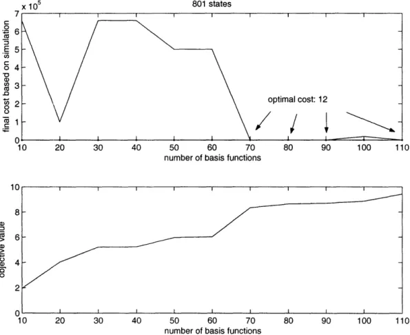
For each given number of basis functions, the ALP yields an approximation J* and a policy is generated based on this value function estimation. The final costs of the simulations are averaged over 5 trials under the same policy. In each trial the maximum number of simulation steps is 100. Within the scope of our experiment, the robot should be able to complete the task within 100 steps given a good policy. After some trial and error on the optimal number of simulation steps, it is found that too large a number gives rise to more variance in the final cost of the simulations but less insight into the performance of our policies. If the robot does not complete the task, it is an indication that it might be stuck in certain states and kept going back

and forth until the end of the simulation, or the policy is suboptimal. The number of

basis functions used increases at increments of 10 in all experiments up to 200. These basis functions are not chosen randomly from a pool. Instead, they are ordered such that the set of 10 bases used is also used in the set of 20; the set of 80 bases used is also used in the set of 90 and so on. Therefore, the change in objective value of the ALP may be interpreted as the effectiveness of the basis functions incremented in each run.

4.3.1 Analysis of Object Value Plots

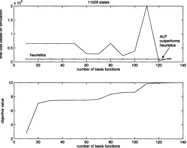
The plots of objective value of the ALP, though monotonically increasing, are not very smooth. It is observed that the change in objective value follows a certain pattern,

and this pattern is fairly consistent across problems of different sizes. The increase in objective value due to basis functions 10-20 is the most significant, followed by basis 60-70 and 100-110. The jump in objective value indicates that these basis functions are significant and they span larger part of the value function. Bases 10-20 are feature-based, including time to finishing the task, distance from base station squared, cubed and task progress check and so on. Bases 60-70 are polynomials of state parameters; bases 100-110 are natural logs of polynomials of state parameters. Feature-based basis functions appear to be able to capture the essence of the problems, whereas the effectiveness of other basis functions is not guaranteed and requires more trial and error in formulation.

Since the number of constraints in the ALP equals the number of state-action pairs, as the problem size scales up, the ALP has an enormous number of elements. In our experiments, the ALPs start to become dual or even primal infeasible when more than 120 - 150 basis functions are used, even for a seemingly small problem with several thousand states. The ALP becomes dual infeasible sooner as the problem size

increases. It is likely that the C++ program or the linear programming software

runs into numerical issues when approaching the optimal solution due to rounding errors. This problem points us to the need of constraint sampling discussed in the

Limitations and Improvements section.

4.3.2 Analysis of Value Function Estimation

The value function estimations show significantly larger variance in value and trend than the objective value plots. The "roughness" of cost estimation based on simula-tion may be explained by the following factors:

* Robot breaks down randomly according to a binomial distribution (with prob-ability 0.1 in our case).

* The objective of our ALP minimizes the weighted norm J* -

r*l,,

but

the monotonic increase in objective value does not guarantee the value function

estimation for frequently visited states are getting better, especially if the

state-relevance vector differs from the actual distribution.

* Different kinds of basis functions are being added but their effectiveness are not uniform. We do not know which of these basis functions spans the value function. The improvement in policy is not likely to be linear, nor guaranteed to be a smooth function of the number of basis functions.

4.3.3 Overall Performance of ALP Algorithm

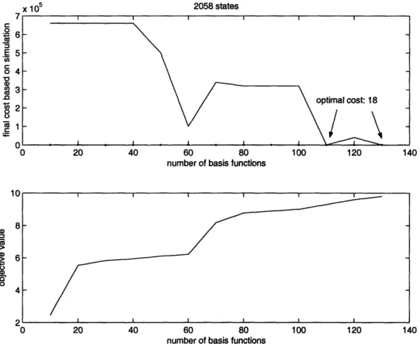
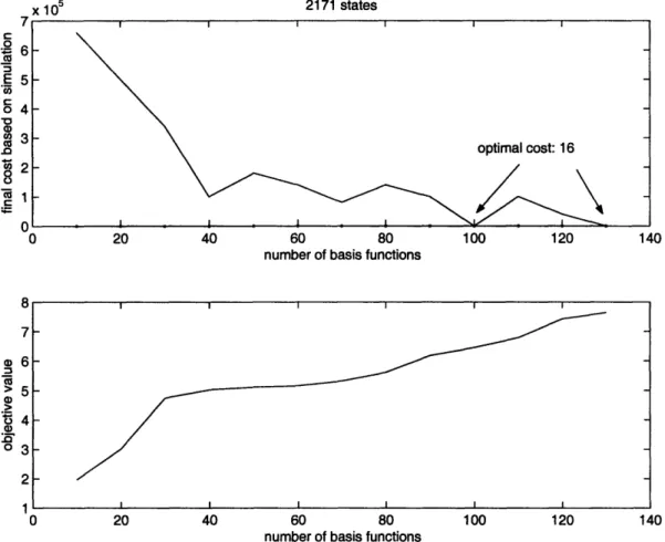
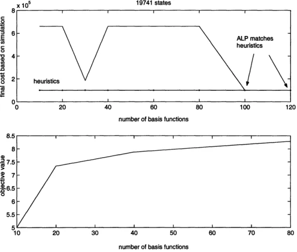
In smaller scale problems (e.g. < 2,500 states) where optimal solution could be found by policy iteration, the value function estimate hits the optimal value after 80 to 90 basis functions on average.

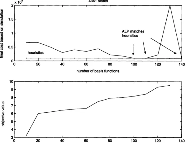
In larger scale problems (e.g 4,000-20,000 states), the value function estimate matches that of heuristics after 100 basis functions on average. Occasionally, the policy from ALP outperforms that from heuristics.

We observe that in all simulations the optimal cost or the benchmark set by heuristics is attained well before the objective value reaches optimality. This result implies that our r is a good estimate of the value function for frequently visited

states. Optimal policies are found fairly quickly with < 100 basis functions even though our objective value is still far from perfect. Moreover, the number of basis functions needed to find the optimal policy does not increase significantly in larger systems. Hence, ALP is an efficient algorithm and scales well with problem size.

4.4 Limitations and Improvements

As the number of basis function increases, the ALP may become dual infeasible due to possible numerical problems and rounding errors. It is found that numerical issues arise mainly when the coefficients in the LP differ widely in orders of magnitude,

which are associated with highly non-linear basis functions and polynomials of very high order. In that case, the primal solution would be very poor and hence the policy generated. Therefore, care must be taken in designing the basis functions and high order polynomials may not be as desirable.

The number of constraints in the ALP equals the number of state-action pairs. As

the problem size scales up, the number of elements increases exponentially. The huge

LP size and the possibility of numerical error render the ALP infeasible. Constraint

sampling methods as discussed in [4] may solve this problem by trying to pick out the more relevant (binding) set of constraints in the ALP according to the state-relevance

distribution.

Without a priori knowledge of the state-relevance distribution, uniform state rel-evance is used in all simulations. However, as the policy improves at successive iterations, we could adjust the state-relevance vector by keeping track of how often a state is visited by the policies. The improvement in state-relevance distribution would benefit constraint sampling and subsequently, cost estimation.

In this experiment, basis functions are added at increments of 10 from an ordered set. In the future, we may design an algorithm that picks the appropriate basis function to be added at each step from a random pool. This way, only the best basis functions are included in our 4I matrix. It is possible that even fewer basis functions would be needed to find the optimal policy of a problem.

Chapter 5

Conclusion

Approximate Linear Programming is a powerful methodology for decision-making in complex systems. This method requires some degree of experimentation in design-ing the basis functions. Results from this experiment show that feature-based basis

functions seem to work the best because they capture characteristics of the problem,

whereas other effective basis functions may only be found by trial and error. Nev-ertheless, monotonic increase in objective value is guaranteed in the ALP no matter what basis functions are used. It may be advisable to create a large pool of randomly generated basis functions and run ALP on a subset of these basis functions at a time, select the best ones and keep iterating using a combination of effective bases from previous iterations and new bases. This way, we may be able to limit the matrix size for fast computations and retain only the best basis functions from each iteration

in our · matrix.

We shall keep in mind that the robotic control problem is used only as a case study of the usefulness and performance of Approximate Linear Programming as a decision-making tool. The study demonstrates that ALP is indeed a promising approach to solving large-scale decision-making problems if the basis functions are carefully designed and selected. It is shown that control policy from ALP at least matches, and sometimes outperforms that of heuristics given a relatively small number of basis functions. Despite issues such as state-relevance estimation and numerical problems that need to be addressed, the encouraging results shed light on the possibility of

Appendix A

Figures

x 105 801 states

number of basis functions

10 8 6 4 2 ,I I I I , I I 10 20 30 40 50 60 70 80 90i 100 1 10 20 30 40 50 60 70 80 90 100 110

number of basis functions

Figure A-i: Objective Value and Value Function Estimate with 801 states

C 0 OFE (0 CD o 0 C.) 0 (D a) a, So_a) 0 I\ U A

X o5 2058 states

0 20 40 60 80 100 120 140

number of basis functions

I I I I I I

0 20 40 60 80 100 120 140

number of basis functions

Figure A-2: Objective Value and Value Function Estimate with 2058 states

C

.E5

o4

n 0 .A 1U 8 a) 0 4 9

x l105 2171 states

number of basis functions

*0

I I I I I I

0 20 40 60 80 100 120 140

number of basis functions

Figure A-3: Objective Value and Value Function Estimate with 2171 states

c ca :3 E 0 co .0 8 co 6 > 5 S 4

03

9 I

4341 states

20 40 60 80 100 120

number of basis functions

20 40 60 80 100 120 140

Figure A-4: Objective Value and Value Function Estimate with 4341 states

x 106 C 0 16 E C 0 u0 (D W (U .00 0c a 1. O. 0 10 140 9 8 7 6 5 4 a) E .90) :U o 3 0

x 106 1 1009 states

0 20 40 60 80 100 120 140

number of basis functions

en'

0 20 40 60 80 100 120 140

number of basis functions

Figure A-5: Objective Value and Value Function Estimate with 11009 states

.O C 1.5 E C o 0D 1 U) .0_co o 0.5 r lU ID ₈ a) a :6₀ 4 9

8 I I I I I I 6 4 2 20 \e ALP matches heuristics

/la

~~n

I I

~I

I I 40 60

number of basis functions

80 100 120 0.0 8 -7.5 a 7 *'6.5 6 5.5 ; 10 20 30

Figure A-6: Objective Value

40 50 60 70

number of basis functions

and Value Function Estimate with 1974

C 0 16 E C 0 'a Cu_co CU .0 0 r-r 0 0 80 1 states x 1o05 19741 states O c

Bibliography

[1] D.P. Bertsekas. Dynamic Programming and Optimal Control, Volume one, Athena

Scientific, 2005

[2] D.P. Bertsekas. Dynamic Programming and Optimal Control, Volume two, Athena

Scientific, 2005

[3] D.P. de Farias. 2.193 lecture notes 1-17 (unpublished) 2005

[4] D.P. de Farias. The Linear Programming Approach to Approximate Dynamic

Pro-gramming: Theory and Application. PhD thesis, Department of Management

Sci-ence and Engineering, Stanford University, June 2002

[5] John Forrest, David de la Nuez, Robin L. Heimer, CLP User Guide, Columbia University & IBM Research, 2004