An algorithm for reducing atmospheric density model errors using satellite observation data in real-time

An Algorithm for Reducing Atmospheric Density

Model Errors Using Satellite Observation Data in

Real-Time

by

Sarah Elizabeth Bergstrom

Bachelor of Science, Swarthmore College, 2000

Submitted to the Department of Aeronautics and Astronautics

in partial fulfillment of the requirements for the degree of

Master of Science in Aeronautics and Astronautics

at the

MASSACHUSETTS INSTITUTE OF TECHNOLOGY

June 2002

©

Massachusetts Institute of Technology 2002. All rights reserved.

A uthor ...

...

Department of Aeronautics and Astronautics

lay 10, 2002

2

Certified by.

...

/Dr. Paul J. Cefola

Technical Staff, the MIT Lincoln Laboratory

Lecturer, Department of Aeronautics and Astronautics

Thesis Supervisor

Certified

by...

_...

Dr. Ron J. Proulx

Prin ipal Member of the Technical Staff,

the Charles Stark Draper Laboratory

Thesis

SuDervisor

Accepted by...

...

Wallace E. Vander Velde

Professor of Aeronautics and Astronautics

Chair, Committee on Graduate Students

MASSACHUSETTS

iSTITUt

OF TECHNOLOGY

THIS PAGE INTENTIONALLY LEFT BLANK

An Algorithm for Reducing Atmospheric Density Model

Errors Using Satellite Observation Data in Real-Time

by

Sarah Elizabeth Bergstrom

Submitted to the Department of Aeronautics and Astronautics on May 24, 2002, in partial fulfillment of the

requirements for the degree of

Master of Science in Aeronautics and Astronautics

Abstract

Atmospheric density mismodeling is a large source of errors in satellite orbit determi-nation and prediction in the 200-600 kilometer range. Algorithms for correcting or "calibrating" an existing atmospheric density model to improve accuracy have been seen as a major way to reduce these errors. This thesis examines one particular algo-rithm, which does not require launching special "calibration satellites" or new sensor platforms. It relies solely on the large quantity of observations of existing satellites, which are already being made for space catalog maintenance. By processing these satellite observations in near real-time, a linear correction factor can be determined and forecasted into the near future. As a side benefit, improved estimates of the ballistic coefficients of some satellites are also produced. Also, statistics concerning the accuracy of the underlying density model can also be extracted from the correc-tion. This algorithm had previously been implemented and the implementation had been partially validated using simulated data. This thesis describes the completion of the validation process using simulated data and the beginning of the real data validation process. It is also intended to serve as a manual for using and modifying the implementation of the algorithm.

Thesis Supervisor: Dr. Paul J. Cefola

Title: Technical Staff, the MIT Lincoln Laboratory and Lecturer, Department of Aeronautics and Astronautics

Thesis Supervisor: Dr. Ron J. Proulx

Title: Principal Member of the Technical Staff, the Charles Stark Draper Laboratory

THIS PAGE INTENTIONALLY LEFT BLANK

Acknowledgments

First, and foremost, I want to thank my thesis advisor at the MIT Lincoln Laboratory (LL), Dr. Paul Cefola.

I'd also like to thank Dr. Ronald Proulx at the Charles Stark Draper Laboratory (CSDL), who has been a part of this research project since its commencement. He has offered continuing encouragement and technical assistance throughout this project, including enormous help with the seemingly-neverending adventures in file transfer between CSDL and LL.

Second, I want to thank George Granholm, Jack Fischer, Prof. Andrey Nazarenko, and Dr. Vasiliy Yurasov for their fine work, upon which all of my endeavours here have depended. Their papers and theses have been a continual source of inspiration and insight into the intricacies of atmospheric density modelling and satellite orbit determination. Thanks especially to George for finding time in his busy schedule with the U.S. Air Force to provide some initial guidance on working with the software.

Thanks go to Lt. Col. David Vallado (USAF) for providing real observation data. At LL, I'd like to extend thanks to Group 98 Leader Dr. Sid Sridharan for supporting this project. I'd also like to thank Jim Apicella and Sherry Robarge for computer support, Zach Folcik for assistance with the gtds-granholm makefiles and various other software, and Gladys Chaput, Kathy Fellows, Bonnie Tuohy, and Nancy Alusow for administrative and travel assistance.

At CSDL, I'd like to thank Darryl Sargent for his help in coordinating the joint work between the Labs. I'd also like to thank Linda Leonard for computer support in the EDCF computing facility.

I'd like to thank Dr. Richard Battin at MIT for cultivating my interest in orbital mechanics and pointing me at this research project. Thanks also go to my academic advisor, Dr. J. P. Clarke, for giving me the freedom to pursue what interested me most, and for assisting with travel arrangements, along with assistance from Jennie Leith and Marie Stuppard.

On a personal level, I'd like to thank my family for their encouragement of all

my academic endeavours. To my best friend Jen - you've always been ahead of me, inspiring me to keep going. To my beloved Dave, thanks for being there for me. To my roommate (and LATEX consultant) Chaos - thanks for putting up with the dishes I didn't wash during the last few weeks of every semester, and for being a great friend.

Contents

1 Introduction 17

1.1 Atmospheric Density Modeling . . . . 17

1.1.1 A Brief History . . . . 17

1.1.2 An Overview of the Entire Atmosphere . . . . 18

1.1.3 Thermosphere Modeling Details . . . . 21

1.1.4 M odel Errors . . . . 23

1.1.5 A New Empiricism . . . . 23

1.2 Prior Work on this Algorithm . . . . 24

1.2.1 Nazarenko and Yurasov's Original Development . . . . 24

1.2.2 George Granholm's Work . . . . 24

1.3 Outline of this Thesis . . . . 25

2 Mathematical Details 29 2.1 Basic Concepts . . . . 29

2.2 Linear Correction Factors . . . . 30

2.3 Ballistic Factors to Correction Coefficients . . . . 31

2.3.1 Fitting Ballistic Factors to Data . . . . 31

2.3.2 Deriving Corrections from Ballistic Factors . . . . 32

2.3.3 Weighted Least Squares . . . . 33

2.3.4 Solution Boundaries . . . . 36

2.4 Forecasting Linear Correction Factors . . . . 37

2.5 Ballistic Factor Estimation . . . . 38

2.5.1 BFE basic process . . . . 38 7

CONTENTS

2.5.2 Derivation for One Standard Satellite . . . .. 39

2.5.3 Multiple Standard Satellites . . . . 43

3 Implementation Overview 45 3.1 Computer Code . . . . 45

3.1.1 G T D S . . . . 46

3.1.2 Atm oC al . . . .. 47

3.2 D ata Flow . . . . 48

4 Simulated Data Validation 51 4.1 Simulated Data Generation . . . . 51

4.1.1 Preparation . . . ... 52

4.1.2 Truth Orbit Generation . . . . 53

4.2 Reproduction of Prior Results using Simulated Data . . . . 55

4.2.1 Data Flow Verification . . . . 55

4.2.2 Differences between Truth and Fit Models . . . . 57

4.2.3 Simulating "Noisy" Observations . . . . 61

5 New Validation Results with Simulated Data 65 5.1 Ballistic Factor Distortion . . . . 66

5.2 R esults . . . . 70

5.2.1 D ata Flow . . . . 70

5.2.2 Effects on Atmospheric Density Correction . . . . 70

5.2.3 Convergence . . . . 73

5.2.4 Update Cycle Length . . . . 73

5.2.5 Height Dependence of Errors . . . . 73

5.2.6 Global Distortion/Correction Effects . . . . 78

5.2.7 Omitting Recalculation of kI Values . . . . 80 8

CONTENTS 9

6 Real Data Validation 83

6.1 Data Preparation ... ... 83

6.1.1 Conversion of B3 Observations . . . . 83

6.1.2 Station D ata . . . . 85

6.1.3 Observation Scheduling . . . . 85

6.1.4 Current Status . . . . 85

7 Conclusions and Future Work 91 7.1 C onclusions . . . . 91 7.2 Future W ork . . . . 91 7.2.1 Further Tests . . . . 92 7.2.2 GTDS Bugs . . . . 93 7.2.3 New GTDS Features . . . . 93 7.2.4 GTDS Integration . . . . 94 7.2.5 AtmoCal Refinements . . . . 94

7.2.6 Major AtmoCal Additions/Changes . . . . 95

A Key to Symbols, Abbreviations, Etc. 99 A.1 Text Conventions . . . . 99

A.2 Expressions and Abbreviations . . . . 100

B Implementation Miscellanea 105 B.1 CVS and Revision Control . . . . 105

B.2 File Names and Locations . . . . 106

B.3 Environment Variables . . . . 109

C GTDS 111 C.1 GTDS Changes . . . . 111

C.2 GTDS Data Files . . . . 113

10 CONTENTS

C.4 List of Known Bugs/Issues ... 129

D Annotated Code 131 D.1 TLE2osc.pl . . . . 132 D .2 genobs.pl. . . . . 141 D .3 distort-bfs.m . . . . 151 D .4 estbfs.pl . . . . 154 D .5 calcvars.pl . . . . 174

D.6 Drivers for estbfs.pl and calcvars.pl . . . . 183

D .7 cale b.m . . . . 191

D .8 D ates.pin . . . . 198

D .9 b3conv.pl . . . . 202

D.10 Other Utilities . . . . 208

D.11 Graphing Utilities . . . . 212

E File Utilities and Formats 219 E.1 B3 to OBSCARD Conversion Utility . . . . 219

E.2 Building New GTDS Binary Files . . . . 222

E.3 Detailed File Formats . . . . 222

E.4 GTDS Input Decks . . . . 225

F IX Notes 231

Bibliography 233

List of Figures

1-1 Atmospheric Regions . . . . 19

1-2 Atmospheric Composition at Low Exospheric Temperature . . . . 20

1-3 Atmospheric Composition at High Exospheric Temperature . . . . 21

1-4 Summary of George Granholm's Work . . . . 25

2-1 Flowchart for Overall AtmoCal Operation . . . . 31

2-2 Visual Representation of the Fit Window for Satellite

j

2-3 Ratio of True Density to Jacchia 1971 Model Density . . . . 34

2-4 Block Diagram for Correction Factor Forecasting . . . . 38

2-5 Flowchart for Ballistic Factor Updating Cycle . . . . 44

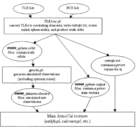
3-1 AtmoCal Operation Flowchart Including File Names . . . . 48

4-1 Flowchart for Simulated Observation Creation . . . . 54

4-2 B-values with No Noise, No Mismodeling . . . . 56

4-3 Linear Atmospheric Density Correction Factors with No Noise, No Mis-m odelling . . . . 56

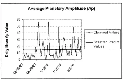
4-4 Observed Daily Mean and Schatten Ap Values for 12/15/99-2/15/00 58 4-5 Daily and Schatten F1 0.7 Values for 12/15/99-2/15/00 . . . . 58

4-6 Observed F1 0.7 and ap Values During Fit Window . . . . 59

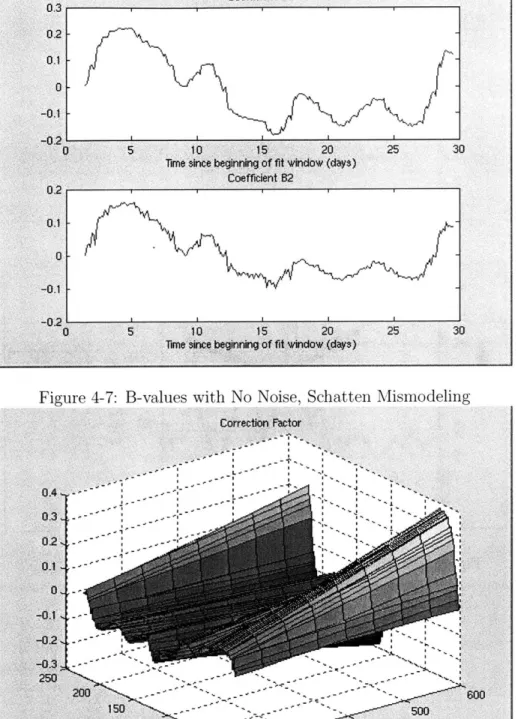
4-7 B-values with No Noise, Schatten Mismodeling . . . . 60 11

LIST OF FIGURES

4-8 Linear Atmospheric Density Correction Factors with No Noise,

Schat-ten M ism odeling . . . . 60

4-9 B-values with Observation Noise, No Mismodelling . . . . 63

4-10 Linear Atmospheric Density Correction Factors with Observation Noise, No M ism odeling . . . .. 63

4-11 B-values with Observation Noise, Schatten Mismodelling . . . . 64

4-12 Linear Atmospheric Density Correction Factors with Observation Noise, Schatten Mismodeling . . . . 64

5-1 Distribution of (undistorted) Ballistic Factors for All Satellites . . . . 67

5-2 Distribution of Ballistic Factors for the Standard Satellites used in BFE validation . . . . 67

5-3 Distribution of Perigee Heights for All Satellites . . . . 68

5-4 Distribution of Perigee Heights for the Standard Satellites used in BFE validation . . . . 68

5-5 Ballistic Factor Distortion Ratios . . . . 69

5-6 BF Percent Errors after Iteration, with No Noise, No Mismodeling, No Initial D istortion . . . . 71

5-7 BF Errors Sorted by Initial BF, with No Noise, No Mismodelling, No Initial D istortion . . . . 72

5-8 Comparison of B-values with and without Initial Ballistic Factor Dis-tortion . . . . 72

5-9 Convergence for five-day case . . . . 74

5-10 Convergence for ten-day case . . . . 74

5-11 Percent Errors for all Satellites before BFE iteration . . . . 75

5-12 Percent Errors for all Satellites after 5 BFE iterations . . . . 75

5-13 Average Absolute Percent Deviation as a Function of Iteration Period (exam ple 1) . . . . 76 12

LIST OF FIGURES

5-14 Average Absolute Percent Deviation as a Function of Iteration Period

(exam ple 2) . . . . 76

5-15 Remaining Errors After Iteration, Sorted by Perigee Height . . . . 77

5-16 BFE iteration with No Global Distortion . . . . 78

5-17 Percent Errors for all Satellites before BFE iteration, with no Global D istortion . . . . 79

5-18 Percent Errors for all Satellites after 5 BFE iterations, with no Global D istortion . . . . 79

6-1 Flowchart for Real Observation Preparation . . . . 84

B-1 File Structure for Large Data Files . . . . 107

B-2 File Structure for AtmoCal and Small Data Files . . . . 107

B-3 File Structure for gtds-granholm . . . . 108 13

LIST OF FIGURES

THIS PAGE INTENTIONALLY LEFT BLANK 14

List of Tables

Statistics for B-values with No Noise, No Mismodeling . . . . Statistics for B-values with No Noise, Schatten Mismodeling . . . . . Statistics for B-values with Observation Noise, No Mismodeling . . . Statistics for B-values with Observation Noise, Schatten Mismodeling 5.1 _{Statistics for Ballistic Factor "Improvements" with No Noise, No}

Mis-modeling, No Initial Distortion B.1 Common CVS commands B.2 Environment Variable List C.1 GTDS Code Alteration List C.2 List of GTDS Data Files . . . D.1 TLE2osc.pl Fact Sheet . . . . D.2 genobs.pl Fact Sheet . . . . . D.3 distort-bfs.m Fact Sheet . . . D.4 estbfs.pl Fact Sheet . . . . D.5 calcvars.pl Fact Sheet . . . . . D.6 runestbfs.pl Fact Sheet . . . . D.7 runcalevars.pl Fact Sheet . . . D.8 bfe-iter.pl Fact Sheet . . . . . D.9 calcb.m Fact Sheet . . . .

. . . . 71 . . . . 106 . . . . 109 . . . . 1 12 . . . . 113 . . . . 132 . . . . 141 . . . . 151 . . . . 154 . . . . 174 . . . . 183 . . . . 183 . . . . 184 . . . . 191 15 4.1 4.2 4.3 4.4 55 57 62 62

LIST OF TABLES

D.10 Dates.pm Fact Sheet ... 198

D.11 b3conv.pl Fact Sheet ... ... 202

D.12 dateconvert.pl Fact Sheet . . . . 208

D.13 get-peri.pl Fact Sheet . . . . 208

D.14 read-b.m Fact Sheet . . . . 212

D.15 analyze-atmcal.m Fact Sheet . . . . 212

D.16 readinitinfo.m Fact Sheet . . . . 212

E.1 List of NORADPP Files Modified . . . . 221

E.2 OBSCARD Format . . . .~. . . . . 223

E.3 Format of initinfo.txt . . . . 224

E.4 Format of jac-densvars.txt . . . . 224

E.5 Format of ballfcts.txt . . . . 224

E.6 Format of Station Card 0 . . . . 227

E.7 Format of Station Card 1 . . . . . . 228

E.8 Format of ATMCAL card . . . . 229 16

Chapter 1

Introduction

1.1

Atmospheric Density Modeling

1.1.1

A Brief History

When Sputnik was launched in 1957 [7], very little was known about the nature of the atmosphere above 100 kilometers. Data from the first high-altitude sounding rockets and satellites in the late 1950's and early 1960's provided enough information for researchers to create elementary models, based mainly on the ideal gas equation and the hydrostatic equation [42]. Most notable among these early models was that of Luigi Jacchia, based in part on earlier models by Marcel Nicolet [23]. In 1977, Alan Hedin published the first of a series of models based on (and named after) Mass Spectrometer and Incoherent Scatter (MSIS) data[19]. The MSIS models are still under active development, with the Naval Research Laboratory's NRLMSISE-2000 being the most recent version[44].

A multitude of other models have also been created since the 1970's, but none, as of yet', has demonstrated any significant improvement over the Jacchia-Roberts 1971

'The cited comparison was performed before MSISE-90 and NRLMSISE-2000 were available. These and other recent models may offer some improvements, although the same modeling difficulties listed in Section 1.1.4 apply.

CHAPTER 1. INTRODUCTION

(JR-71) model [34]. All models seem to show a 10-15% error in quiet and normal conditions, with errors potentially reaching 30% in highly perturbed conditions.

Increasing the accuracy of atmospheric density models would allow satellite orbits to be determined and predicted into the future with higher precision and for longer time periods. This in turn allows for more efficient planning of maneuvers, including routine stationkeeping as well as collision-avoidance, de-orbiting, or maneuvers to transition between two orbits. Collision avoidance is especially important now that the International Space Station (ISS) orbits in the 300-400 kilometer region[58].

1.1.2

An Overview of the Entire Atmosphere

Most people are only familiar with the lowest region of the atmosphere, called the troposphere, which extends for the first 11 kilometers above the Earth's surface. All weather takes place in this region, and it behaves according to simple, intuitive prin-ciples. As one ascends through the troposphere, the air gets colder, since the main source of heat in this region is the surface of the Earth, and thinner, due to decreased gravitational forces, but remains relatively similar in composition. (All of the regions of the Earth's atmosphere are summarized in Figures 1-1, 1-2 and 1-3.)

Beyond the troposphere, the temperature begins to rise again, due to the effects of solar radiation on atmospheric oxygen. Some components of ultraviolet solar radiation split molecular oxygen (02) into atomic oxygen (0) and ozone (03), while others are absorbed by the ozone and heat both the ozone molecules and the surrounding air. This region, formally called the stratosphere, familiar to most people as "the ozone layer" extends upwards to approximately 50 kilometers, where the ozone heating effect no longer dominates, and the temperature begins to drop once more. This region of decreasing temperature, known as the mesosphere, extends to approximately 90 kilometers, whereupon solar radiation heating again begins to dominate. Everything above this final temperature inflection point, known as the mesopause, is referred 18

1.1. ATMOSPHERIC DENSITY MODELING 19

to as the thermosphere, because of the extremely high temperatures2 _{reached in the}

region. The various regions of the atmosphere and average temperature are shown in Figure 1-13.

Troposphere Stratopause Homopause exospheric temperature

200 100 300( 200 100 varies from 600 to 20000K,

Tropopause Mesopause depending on time/season

0-Stratosphere Mesosphere Thermosphere>

Homosphere Hetemosphere

0 20 40 60 80 100 300 600 900 1201

Height (km)

Figure 1-1: Atmospheric Regions

Two other regional divisions are often found in atmospheric modeling literature: the ionosphere, which refers to the region of the atmosphere containing ionized parti-cles (roughly equivalent to the thermosphere), and the exosphere, which is the entire atmosphere above the exobase, which is the point at which individual gas atoms may be thought of as being in individual orbits around the earth. The exospheric temper-ature is the tempertemper-ature that is asymptotically approached in the exosphere as the height increases to infinity, as seen in Figure 1-1.

Another important division of the atmosphere occurs around 100 kilometers, where the composition of the atmosphere begins to change. Below this point, known

2

Note that a strict, scientific definition of "temperature", based on the kinetic energy of individual gas molecules, must be used in this region, since gas densities are so low that a thermometer would be useless.

3

20 CHAPTER 1. INTRODUCTION

as the homopause, the atmosphere contains the familiar mix of 78 percent nitrogen

(N2), 21 percent oxygen (02), 1 percent argon (Ar), with trace amounts of water

vapor and other compounds. Around the homopause, the air becomes thin enough that particle collisions become rare. This has two effects: first, atomic oxygen be-comes a major component, since the atoms rarely collide to reform 02, and mixing no longer keeps the proportions of various components steady. Instead, the particles of each component gas react individually to the Earth's gravitational field, and the components stratify by molecular weight. Approximate individual concentrations4 in the 200-600 kilometer range are shown below for lower and upper extreme exospheric temperatures (500 and 1900 'K) 5.

Exospheric Temperature 500*K

2

-1

Temperature

Figure 1-2: Atmospheric Composition at Low Exospheric Temperature

Normal daytime temperatures are in the 1500-2000 'Krange, and nighttime tem-peratures during quiet periods fall in the 500-700 'Krange. Thus, values close to or at the extremes shown in Figures 1-2 and 1-3 tend to be seen on a daily basis, with the density at any particular altitude in the thermosphere fluctuating by several hundred percent.

4

Hydrogen is not included in the JR-71 model below 500 kilometers.

5

Figure 1-2 uses data from pages 78-79 and Figure 1-3 uses data from pages 106-107 of Jacchia's 1971 model [25].

1.1. ATMOSPHERIC DENSITY MODELING 21 Exospheric Temperature 1900'K

2

~1600

~~~

Figure 1-3: Atmospheric Composition at High Exospheric Temperature

1.1.3

Thermosphere Modeling Details

Most modern thermospheric density models include several major factors:

Lower Boundary Conditions: Thermospheric models must have a starting point, and most start at altitudes between 90 and 120 kilometers, setting either con-stant or seasonally-dependent boundary conditions[25, 17]. (The E (for Ex-tended) in the MSISE-series models denotes that a model for the lower atmo-sphere has been linked to these boundary conditions from the other side, but we are only concerned here with the thermospheric model.)

Diurnal Variation: This is simply the exospheric temperature difference between day and night. The maximum density increase due to the sun's heating effect occurs around 2 pm local solar time, at a latitude known as the sub-solar point, and the minimum around 3 am. The strength of this effect and the location of the sub-solar point varies seasonally, and is well-understood[25].

Annual and Semi-annual Variations: There are several seasonal atmospheric composition changes, including the winter helium bulge and some low-altitude hydrogen variations. The hydrogen variations are sometimes modeled as tem-perature variations for simplicity and compatibility with boundary conditions.

CHAPTER 1. INTRODUCTION

These phenomena are well measured, although the accuracy to which they are modeled varies, especially at lower altitudes[25].

Solar Activity Variations: Extreme ultraviolet (EUV) radiation from the sun is the primary source of heat in the thermosphere, and the amount of radiation produced by the sun varies greatly over the 11-year solar cycle and with sunspot activity. Since no appreciable amount of the EUV wavelengths which cause heating reach the surface of the earth, we rely on measurements of the solar radio flux at a wavelength of 10.7 cm (which is a frequency of 2800 MHz). This radio flux is known as the F10.7 index, and is usually tabulated on a, daily basis,

along with the average flux (F1 0.7) seen over the preceding 90 or 180 days. The

F10.7 index is used to determine short-term variations due to sunspots and other

temporary solar phenomenon, while F1 0.7 gives a measure of the average flux seen during that portion of the 11-year solar cycle. Past values of F1 0.7 from the appropriate time in the solar cycle can be used to create lists of predicted F10.7

values. Ken Schatten designed one such prediction method, details of which can be found on his web site[49]. Measurements of the actual EUV radiation taken from various upper-atmospheric experiments in the 1960's and 1970's were used to determine that the F10.7 and F1 0.7 indices are more accurate than the Call K plage index or visible sunspot observations. [33]

Geomagnetic Activity Variations: Geomagnetic storms, caused by coronal mass ejections and other solar eruptions create strong short-term density fluctua-tions[57]. The planetary geomagnetic index ap (or the closesly related index Ky) is used as the indicator for these effects. The ap index is usually tabulated as a smoothed daily average, and the K, index is not smoothed (and is tablulated every 3 hours), and both are useful in density calculation [36].

1.1. ATMOSPHERIC DENSITY MODELING

1.1.4

Model Errors

The solar and geomagnetic activity variations discussed in the preceding list are the effects that give rise to the greatest errors in atmospheric density determination and prediction. First, F10.7, F10.7, ap, and K, are not perfect indicators of the underlying

effects. Attempts to replace both of them are underway, but no replacements have yet been widely adopted[44, 52]. Second, none of the methods for predicting future values of these indices are able to capture the random nature of unexpected sunspots or coronal mass ejections.

1.1.5

A New Empiricism

Observational data has always been at the core of atmospheric density models, but it was not until the past decade, when sufficient computer speed and storage capabil-ities became available, that the idea of improving models by incorporating real-time data from large numbers of satellites became popular. The hope is that the so-called 15% (one-sigma) barrier can be broken consistently by using this algorithm or an-other"calibration method" [36]. This project is one of several in this field - the High Accuracy Satellite Drag Model (HASDM) is another, and Frank Marcos also has a project in this area[51, 35]. One major alternative to the "calibration" method is the use of satellites with direct atmospheric drag and/or composition observation capabilities, instead of relying solely on ground-based data. Current projects in-clude the CHAMP and GRACE satellites, which are both near-spherical and carry high-accuracy accelerometers, and the DMSP satellite, which measures atmospheric density and composition, and the TIMED satellite, which will measure EUV radiation directly[36]. These projects, however, are costly, while the "calibration" methods re-quire only a small amount of processor time, using data that is already being collected for space catalog maintenance.

CHAPTER 1. INTRODUCTION

1.2

Prior Work on this Algorithm

1.2.1

Nazarenko and Yurasov's Original Development

This algorithm was originally developed and tested by Andrey Nazarenko and Vasiliy Yurasov in the early and mid-1990's. In 1997, the Charles Stark Draper Laboratory (CDSL) commissioned a report detailing the latest implementation of Nazarenko and Yurasov's work[41]. This report for CSDL provided both theoretical and empirical support for the algorithm, which appeared both promising and portable.

1.2.2

George Granholm's Work

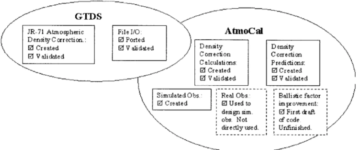
The algorithm was re-implemented from scratch beginning in 1999 by George Gran-holm at CSDL[13]. This new implementation used the Goddard Trajectory Determi-nation System (GTDS)[14] to calculate satellite trajectories (and atmospheric den-sities), on a SGI-UNIX platform. JR-71 was chosen as the underlying atmospheric density model since it was already fully implemented in GTDS, is considered to be one of the most accurate models available, and is in common usage. George im-plemented the atmospheric density correction algorithm by creating a series of Perl scripts that automatically run GTDS and several MATLAB routines (also written by Granholm). To verify that his implementation was functioning properly, he created simulated testing data, and proved that the main components of the algorithm were operating properly. The flowchart in Figure 1-4 shows the sections that Granholm wrote, completed and/or validated. The dotted lines denote sections that Granholm began, which were not completed due to time constraints.

In March 2001, Dr. Paul Cefola, who had been one of the major investigators of the atmospheric density correction project at CSDL, retired from CSDL and assumed a position at the MIT Lincoln Laboratory (LL). Subsequently, in May 2001, LL technical staff met with the CSDL technical and project office staff, and an agreement was made that the project should become a joint CSDL-LL venture.

1.3. OUTLINE OF THIS THESIS 25

GTDS

JR-71 Atmospheric File I/O: AtnoCal DensityCorrection.: 21 Potted

0 Created 1 V alidated D ensity D ensity

0 V alidated Correction Correction

C alculations: Predictions: (9 Created 0 Created 10 Validated El V alidated

SimulatedObs: Real Obs Ballistic factor 0 Created El Used to impr ovement:

design sim. El First draft obs. Not of code. directlyused. Unfinished.

Figure 1-4: Summary of George Granholm's Work

During the summer of 2001, the code was moved by the author and Ron Proulx to the Pisces SGI-UNIX machine at LL, and was given the name AtmoCal.

1.3

Outline of this Thesis

The following outline is intended to serve as an index for finding particular information in the remainder of this thesis.

Chapter 1: Introduction details the motivation and the history of this project. Chapter 2: Mathematical Details includes the derivation of all of the equations

used in the atmospheric density correction process. The first part (Sections 2.2-2.3.4) derives the main atmospheric density correction algorithm, the second (Section 2.4) describes the current techniques used to predict the correction factors into the future, and the third (Sections 2.5.1-2.5.3) derives the ballistic factor improvement algorithm.

Chapter 3: Implementation Overview gives a brief description of the current software implementation of the algorithm detailed in Chapter 2. Details of the computer code are left to the appendices.

CHAPTER 1. INTRODUCTION

Chapter 4: Simulated Data Validation describes and gives results from the sec-tions of George Granholm's simulated data validation process which were re-created on the Pisces machine at LL. It also includes an overview of how the simulated data was generated.

Chapter 5: New Validation Results with Simulated Data shows the results of validating the ballistic factor updating algorithm with simulated data.

Chapter 6: Real Data Validation gives an overview of the process of running AtmoCal on real data.

Chapter 7: Conclusions and Future Work summarizes the current state and the future goals of this project.

Appendix A: Key to Symbols, Abbreviations, Etc. lists all of the mathemat-ical symbols, abbreviations, acronyms, and text conventions used in preparing this thesis.

Appendix B: Implementation Miscellanea describes the use of the Concurrent Version System (CVS) for configuration management and gives information on file locations and shortcuts needed for running AtmoCal.

Appendix C: GTDS describes Granholm's alterations to GTDS and the validation process, which was repeated at LL. This appendix also includes a list of the GTDS binary and text data files used while running AtmoCal.

Appendix D: Annotated Code contains the full text of each of the AtmoCal rou-tines. It also includes tables of user options for AtmoCal rourou-tines.

Appendix E: File Utilities and Formats describes the utility for converting NO-RAD B3 observations to OBSCARD format and lists the formats of all of the AtmoCal I/O files.

1.3. OUTLINE OF THIS THESIS 27

Appendix F: I4TEX Notes includes information on the creation of this thesis. Bibliography lists all of the works consulted in preparing this thesis.

28 CHAPTER 1. INTRODUCTION

Chapter 2

Mathematical Details

2.1

Basic Concepts

A wealth of data is constantly being collected on every object in orbit around the Earth. This data is used to maintain the U.S. space catalog, determine desired orbit corrections, and predict collision risks. The goal of this and other atmospheric density correction methods is to provide a "correction factor" of some sort, which improves an existing atmospheric density model. The correction factor could then be used by anyone using the same density model, in order to improve satellite orbit determination and prediction.

Thus, we need to find a simple and robust way to extract information about the errors of the atmospheric density model from observations of multiple satellites. Once the errors can be quantified, a correction factor that removes or reduces them can then be determined. The algorithm detailed in this thesis, as it is currently operational, provides a linear correction factor for the JR-71 model, using data from over 300 satellites in low earth orbit (LEO).

30 CHAPTER 2. MATHEMATICAL DETAILS

2.2

Linear Correction Factors

The algorithm operates by determining a linear density correction for every three-hour span where sufficient data' is present, and then predicting those correction factors, in three-hour spans, into the near future. The time period of three hours was chosen because it was long enough to accumulate sufficent data under normal conditions. If more data becomes available, this period could be shortened. A linear model was chosen by Nazarenko and Yurasov because it would not try to extract too much information from the data,, but would model the observed errors reasonably well. Thus, we want to determine some linear coefficients bij and b2j that describe

the best correction factor in a given three-hour interval. Designating satellite height by h, the fundamental linear correction equation for the three-hour span tj is:

correction (h, tj) = bij + b2j (h - 400) (2.1) 200

Aside from the observational data (in range/azimuth/elevation format) , the al-gorithm requires only tabulated values of the ballistic factor of each satellite in the catalog. The a priori values for the ballistic factors should be the best ones available when correction begins. (The improvement of ballistic factor estimates is described in Section 2.5. Note that the definition of ballistic factor2 _{used in this paper is:}

CDAx (2.2)

2m

For each three-hour period, then, we want to calculate the correction factor that best approximates the actual difference 6p between the model density pm and the true density p.

'To be precise, 35 data points, in the form of observed ballistic factors, are required for each 3-hour span. The description of how those ballistic factors are created and processed is detailed later in this chapter.

2_{The AtmoCal software performs conversions between the tabulated values of k and Ax in meters}

and Ax in kilometers and mass m when required for the use of GTDS, using a standard value of 2.2

2.3. BALLISTIC FACTORS TO CORRECTION COEFFICIENTS

p = m + =O PM 1+ 6P) (2.3)

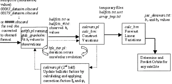
The entire operation of the algorithm can be summarized in the flowchart in Figure 2-1:

b, and b2

b, and bz values (real or simulate list of I values values with including

with associated associated future RangefAzB Determine timesLandiheit _{Construct Forecast}

imes

form at cmdidalW"Ln r501iea

4 values. ... ... Variations

* iteration occxs

ance/solar revoluti

Determine and

Up date ballistic factors by Pre dict Orbits for c al culating and applying any satellite corr ection factors

6

Figure 2-1: Flowchart for Overall AtmoCal Operation

2.3

Ballistic Factors to Correction Coefficients

2.3.1

Fitting Ballistic Factors to Data

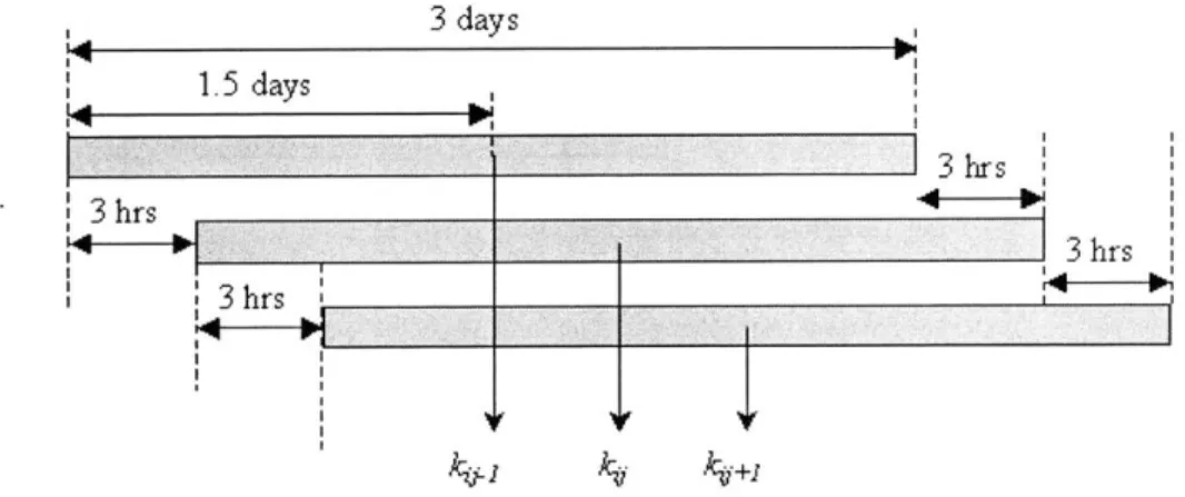
Ballistic factors are determined by fitting orbits to three-day blocks3 of the observa-tional data. GTDS uses the tabulated ballistic factor as an initial guess, and iterates to find the state vector and the observed ballistic factor. This observed ballistic factor k is attributed to time

j,

3

In highly perturbed conditions, or when data is sparse, the three-day window can easily be

lengthened to five days or more.

4

This is a batch-fit method, and was chosen both for consistency with Nazarenko and Yurasov's implementation, and for software simplicity. Granholm discusses the possibility of using recursive methods in Chapter 2 of his thesis, but this capability has not yet been incorporated into AtmoCal.

32

CHAPTER 2. MATHEMATICAL DETAILS

data collection and the first linear correction factor, as well as a 1.5 day gap between the last observation-based (as opposed to prediction-based) correction factor and the end of the data. Any fit runs that do not converge or have a high convergence error at the end of the GTDS run are thrown out, since the remaining observations should be sufficient. 3 days 1. 5 days - - - P 3 hrs 3 hrs _ _ _ _ _ _

I

~I1I

4,.

k~.

Figure 2-2: Visual Representation of the Fit Window for Satellite

j

2.3.2

Deriving Corrections from Ballistic Factors

The derivation of an expression for 6 begins with the equation for the period rate'_OM of a satellite's orbit. Note that f(x) is some unspecified function (connected to the equations of motion) of the state vector x of orbital elements6.

(2.4)

This equation can then be rewritten in terms of the observed ballistic factor and the model density, with the assumption that the observed orbital elements closely match the actual ones.

5_{Any orbital element that is directly related to the energy of the orbit may be substituted for}

period rate, yielding a similar derivation.

6

Any set of orbital elements which fully describe the motion of the satellite is acceptable.

2.3. BALLISTIC FACTORS TO CORRECTION COEFFICIENTS

TO = k - pm(h, tj) -m

f(x)

By dividing Equation 2.4 by Equation 2.5, and assuming that the observed period rate is a good approximation of the actual period rate (i.e. 1j ~~ Tj) an expression for -- in terms of the observed and actual ballistic factors is obtained.

PM ki .p(h,ti) ₁ T i k -pm(h,tj)

I

2.3.3

Weighted Least Squares

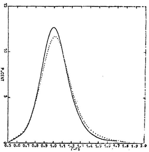
Now, we have a long list of density corrections expressed as ballistic factor ratios, each associated with a time and height. To convert these into single three-hour linear corrections requires some sort of fitting algorithm. Jaeck-Berger and Barlier showed that the errors in Jacchia's 1971 (J71) model are approximately zero-mean and Gaussian. Figure 2-3, reprinted from their work[27], demonstrates this adequately. The dotted line is the normal J71 model, while the solid line is a modified version of J71 described in Jaeck-Berger and Barlier's paper. Both have an approximately normal distribution, with a mean of one, implying that errors of the form 6p =

-P

are also normally-distributed, with a mean of zero. Since the JR-71 model differs from J71 only in the mathematical methods used to calculate several quantities (the JR-71 model was designed to reduce computation time and the size of the required data tables), the results for J71 also apply to JR-71[25, 48].

Since the average error in the density model is zero, a weighted least-squares method provides an appropriate fit. For this method, each error term is defined as:

34 CHAPTER 2. MATHEMATICAL DETAILS

T 1 1 Ir r I u i p

S Pe

Figure 2-3: Ratio of True Density to Jacchia 1971 Model Density

ki h - - 400

'Aij

=

-I -

byj + b2;

(2.7)

ki 200

The A-terms are grouped into a matrix:

A

_Ij

Aj = i(2.8)

S to

2.3. BALLISTIC FACTORS TO CORRECTION COEFFICIENTS

the weighting matrix reflects this7_.

1

W*

(2.9)

02_Mr

Next, we define two matrices, F and B, which together give the linear correction equation detailed in Equation 2.1.

- 400)/200

- 400)/200

b ul

b2jJ

Lastly, we define a matrix aj of the ballistic factor ratio terms.

Ic)- 1

cm) - 1

We can then write a cost function using the matrices defined in the previous equations:

I(bj)

A W

_{Aj = (aj}

Fjbj)TW(aj

Fjbj)

'Standard and non-standard satellites are treated identically in this step, since the tabulated ballistic factor variances already reflect that standard satellites have better-known characteristics. See Section 2.5 for the definitions of standard and non-standars satellites, and for details on reducing the variances for non-standard satellites.

1 (h

1

bj=

(k /

36 CHAPTER 2. MATHEMATICAL DETAILS

6j

(FfWFj)

Ff Waj

These linear correction factors are constant throughout their respective three-hour spans, and change only with height. Latitude and longitude are not included. Like the decision to use only a linear, rather than a second or higher-order model, this choice was made by Nazarenko in order to avoid attempting to extract too much information from limited data. If location-dependent phenomena dominate the remaining errors when such a correction is applied, and sufficient data is available, this limitation should be re-examined.

2.3.4

Solution Boundaries

Any values in aj that exceed a certain tolerance (usually 3-sigma) are discarded before the least-squares solution is carried out. This should discard any outlying values, possibly due to flawed data. Another test is performed by placing a tolerance on the p value GTDS gives as a measure of convergence. Since a large amount of data is available, it seems preferable to simply throw out any questionable points.

Boundaries have also been set on how large these linear correction factors can be [13, 41]. These boundaries are based on the fact that a maximum of 30% error at low altitudes, and a factor of two error at high altitudes seem appropriate based on observations of errors[34]. These rules yield the following boundary equations (at time t):

= b - by E (-0.3, 0.3) (2.15)

Pm h=200

6P = b + b2j E (-.5, 2.0) (2.16)

2.4. FORECASTING LINEAR CORRECTION FACTORS

2.4

Forecasting Linear Correction Factors

The next section of AtmoCal is that which predicts these correction factors into the near future. Since the prediction equations are identical for byj and b2j , the generic variable x(t) will represent either of them in this section. The linear correction factors by and by are both modeled as measurements of independent stochastic processes. First, each "process" is split into a random and a deterministic component:

x(t) = Xd(t) + Xr (t) (2.17) The deterministic component is then modeled as a sum of sinusoids8, with

A

T

and T ~ 27 days (one solar rotation):

d (to)

Xd(t) = T

+

+

A

stationary Gaussian random process, with the correlation function Kx,(T) and power spectral density Sxrxr(s) as follows:

Kx,(T) = o' - ea (2.19)

2o a

SXr, (S) - 2 - 2 (2.20)

az - s

Nazarenko and Yurasov empirically determined that o2 should be in the range 0.1-0.6, and a should be .241/day[40]. A scalar Kalman filter can then be used to project the random component into the future, as a function of to, the last recorded time.

8

This equation can easily be modified if any major, non-sinusoidal, patterns begin to appear in the corrections, but for now appears suitable.

CHAPTER 2. MATHEMATICAL DETAILS

2r(t) = e-"t t') - :r(to) (2.21)

This entire operation can also be represented as a block diagram, shown in Figure 2-4.

Gaussian 202 a

white --- H(s) =X

noise

Figure 2-4: Block Diagram for Correction Factor Forecasting

2.5

Ballistic Factor Estimation

2.5.1

BFE basic process

The ballistic factor updating cycle, which is delimited in Figure 2-1 with dotted lines, is the only section of AtmoCal that does not need to run in near real-time. It requires a larger amount of computer space and time, since it must process a span of observations totalling much more than three days. Some ways to reduce the amount of computer resources required will be discussed in Section 7.1. Since this process only needs to be run occasionally (normally once per 27-day solar rotation), it is usually not a problem to allocate the resources required. After the updated ballistic factors are available, they are incorporated into the real-time orbit determination and prediction section.

The first step in improving ballistic factor estimations is the separation of the satellites in the catalog into two groups: "standard", and "non-standard". Standard satellites have well-known, invariant ballistic factors and masses, and should make up 5-10% of the satellites used. Non-standard satellites may have less well-known 38

2.5. BALLISTIC FACTOR ESTIMATION

and/or slowly varying characteristics. (Observations of objects with highly erratic or completely unknown ballistic factors, including debris and satellites undergoing reconfiguration, should be omitted entirely from those used in the atmospheric density correction process. Satellites with abnormally high eccentricity values should also be omitted. These satellites can still benefit from using the corrected atmospheric density model, but should not be included in its creation.) The tabulated ballistic factors for standard satellites will not be changed by the ballistic factor updating cycle.

2.5.2

Derivation for One Standard Satellite

The ballistic factor updating equations are presented first for the case where there is only one standard satellite. This simplifies the derivation, and the equations can then be easily adapted for multiple standard satellites. The heart of the ballistic factor updating algorithm is the use of "quality factors", or Q-factors, which are used to determine how much an individual ballistic factor should be modified to more closely match the results from other satellites. Nazarenko and Yurasov tested five different Q-factors, and the one used in AtmoCal was the one empirically proven to be most effective. The A error values below are the same ones defined in Equation 2.7.

First, we define a Q-factor in terms of the error terms for the standard satellite.

QS

N, = the set of time spans that contain observations of standard satellite s.

IN,|

Then, using the same format, we define a Q-factor for each non-standard satellite. 39

40 CHAPTER 2. MATHEMATICAL DETAILS

EAni

Q jEN

(2.23)

|Nn|

N, =the set of time spans that contain observations of non-standard satellite n.

INnlI

First, we want to use these Q-factors to find a global correction factor , which will remove any overall bias in the tabulated ballistic factors of all of the non-standard satellites. Such biases are included in the simulated data validation, although it seems unlikely that a clear-cut division between standard and non-standard satellites would appear in real data. (If no such bias exists, the following formulas can still be applied without changing the tabulated ballistic factors, since ( will equal 1. If the inclusion of the global correction factor appears to be slowing convergence, it can be turned off with a software option.) In the following formulae, k, is the actual, unknown ballistic factor of non-standard satellite n, and k-, is the a priori tabulated value.

kn kn (2.24)

To obtain this global correction factor, we begin with the equations for the resid-ual sum of the errors for all non-standard satellites and standard satellites. Since atmospheric density errors are assumed to be zero-mean (see Section 2.3.3), these sums must equal zero, whether we use the tabulated or observed ballistic factors to calculate them. Note that byj and b2j denote the ideal correction factors, while b1 and

bq

For non-standard satellites and empirical measurements: (2.25)

k~-

bE +n bY"20 =EA7j 0

2.5. BALLISTIC FACTOR ESTIMATION

For non-standard satellites and ideal corrections: (2.26)

E

E

b + b2j

h

-

Aj

0

jEN,

k

(

For the single standard satellite and ideal corrections: (2.27)

k -h6 _{- 400}

-

(b

+

200

))

ZA

0

jENs jENs

By substituting Equations 2.25 and 2.26 into Equation 2.24, we obtain the follow-ing relationship:

hn - 400 hn - 400

6

- 1(j + b2j

200

=)

by + by

jEN, j eNn

The global correction factor approximately represents the bias of the variation model caused by the bias of the tabulated ballistic factors9_{. Each biased non-standard}

ballistic factor moves the calculated atmospheric density correction factor away from the ideal variation. Thus, the ideal correction factors are related to those observed by the standard satellite by the following equation:

E- s b + bj

(

400

(by

+

400

Combining Equations 2.27 and 2.29, we get:

9_{The extension of this approximation to multiple standard satellites is based partly on the fact}

that standard satellites make up only a small fraction of the list of satellites being used for atmo-spheric density correction. If this is not the case, this equation should be re-examined. The addition scaling factor based on the percentage of standard satellites in the catalog may be required.

CHAPTER 2. MATHEMATICAL DETAILS

jEN

+ b

hsN

-400

( - E by +b 200

E

j ENs j ENs

Subtracting

EjEN

(hj24

kj -b(hs - 400 j (h_ - 400)

- bj + bq 200

/

j ENs jEN Ns jE Ns

Substituting the expression for

Q,

+

1+

-

INI

(2.32)

j ENS

(b&

We then turn to the individual satellite correction factor, which is determined from the average bias between an individual satellite's k-value and those of all of the non-standard satellites. The derivation is derived in an identical fashion to the derivation of ( above, and is not repeated here. The resulting individual correction factor @, is:

kF = n - k (2.33)

Qn - |Nn|

1nNS 1j + b (hji4O (2.34)

EEN,

+

This entire operation is summarized in Figure 2-5.

Nazarenko determined that 3-4 iterations (with a cycle length of 20 or more days) were normally enough to ensure convergence, and that convergence is improved if the global correction factor is only applied on the first iteration. This makes logical sense, since there should be sufficient data in the initial cycle to remove a simple bias in the

2.5. BALLISTIC FACTOR ESTIMATION

table. AtmoCal is normally set to operate in this fashion, although that behavior can be easily changed.

2.5.3

Multiple Standard Satellites

Expanding the ballistic factor algorithm to include multiple standard satellites is very straightforward. The single

Q,

F(h):

F(h) = ai + a2* h -200 (2.35)

200

Each individual

Q,

the entire update cycle. An unweighted linear least-squares fit is used to fit F(h) to the list of

Q,

Q,

CHAPTER 2. MATHEMATICAL DETAILS

Begin iteration _:

raw observations n kange/Az/El format

initinfo_#txt file containing current "best estimates" ofk and oj. Fit orbits to data (using GTDS), to determine

ballistic factors k.

list of ky values

Perform least-squares fit (Eq. 12), with aj as weights, to find correction values b and

b

from

k4

list oftime-ordered i, and i2, values

Calculate residuals (Ad) and

Q.,

4j

intermediate k values

Recalculate residuals and calculate

Q,

Calculate new variances aj (Eq. 29)

initinfo#_+Ltxt file containing updated estimates of ki and o.

Return to top, using the same raw observations, but new value s of ki and oj.

Figure 2-5: Flowchart for Ballistic Factor Updating Cycle 44

Chapter 3

Implementation Overview

3.1

Computer Code

George Granholm chose to use Perl as the main language for AtmoCal, since it is especially good at handling file input/output and UNIX process control. The ability to spawn multiple subprocesses allows AtmoCal to run more quickly on a multi-processor computer, since multiple copies of GTDS can run at once, on different processors. Perl is more user-friendly and tolerant of slight differences in input file format than languages like FORTRAN and C, and is far more flexible and portable than using UNIX shell scripts. Perl also does not need to be manually recompiled when changes are made, which means that small changes can be made in one script without needing to recompile and relink the entire set of AtmoCal routines. For these reasons, Perl was chosen for AtmoCal, and is generally the language used to create

"wrappers" for older FORTRAN programs[59].

Matrix algebra in Perl is facilitated by using the MatrixReal module, but detailed analyses and statistics are still clumsy in Perl. Thus, MATLAB was used for the in-depth mathematics involved in calculating and predicting the byj and b2j

atmo-spheric density correction coefficients. Several MATLAB scripts were also created for analyzing and graphing results, and have been included in AtmoCal.