Phenomena occurring during cyclic loading and fatigue tests on bituminous materials : Identification and quantification

(1)

HAL Id: tel-01599933

https://tel.archives-ouvertes.fr/tel-01599933

Submitted on 2 Oct 2017

HAL is a multi-disciplinary open access archive for the deposit and dissemination of sci-entific research documents, whether they are pub-lished or not. The documents may come from teaching and research institutions in France or abroad, or from public or private research centers.

L’archive ouverte pluridisciplinaire HAL, est destinée au dépôt et à la diffusion de documents scientifiques de niveau recherche, publiés ou non, émanant des établissements d’enseignement et de recherche français ou étrangers, des laboratoires publics ou privés.

tests on bituminous materials : Identification and

quantification

Lucas Babadopulos

To cite this version:

Lucas Babadopulos. Phenomena occurring during cyclic loading and fatigue tests on bituminous materials : Identification and quantification. Mechanics of materials [physics.class-ph]. Université de Lyon, 2017. English. �NNT : 2017LYSET006�. �tel-01599933�

(2)

N°d’ordre NNT : 2017LYSET006

DOCTORAL THESIS OF THE UNIVERSITY OF LYON

prepared at

Ecole Nationale des Travaux Publics de l’Etat

Doctoral School N° 162

Mécanique, Energétique, Génie Civil et Acoustique (MEGA)

Specialty

:

Civil Engineering

Publicly defended the 15th_{of September 2017 by:}

Lucas Babadopulos

Phenomena occurring during

cyclic loading and fatigue tests

on bituminous materials:

Identification and quantification

before the committee composed of:

DJERAN-MAIGRE, Irini Prof., INSA Lyon President AIREY, Gordon Prof., University of Nottingham, UK Reviewer SOARES, Jorge Barbosa Prof., Federal University of Ceará, Brazil Reviewer BAAJ, Hassan Dr., University of Waterloo, Canada Examiner POUGET, Simon Dr., EIFFAGE Routes Examiner DI BENEDETTO, Hervé Prof., University of Lyon/ENTPE Advisor SAUZÉAT, Cédric Prof., University of Lyon/ENTPE Co-advisor

(3)

N°d’ordre NNT : 2017LYSET006

THESE de DOCTORAT DE L’UNIVERSITE DE LYON

opérée au sein de

l’Ecole Nationale des Travaux Publics de l’Etat

Ecole Doctorale N° 162

Mécanique, Energétique, Génie Civil et Acoustique (MEGA)

Spécialité / discipline de doctorat

:

Génie Civil

Soutenue publiquement le 15/09/2017, par :

Lucas Babadopulos

Phénomènes apparaissant dans les

matériaux bitumineux

lors de chargements cycliques

et d’essais de fatigue :

Identification et quantification

Devant le jury composé de :

DJERAN-MAIGRE, Irini Prof., INSA Lyon Présidente AIREY, Gordon Prof., Université de Nottingham, RU Rapporteur SOARES, Jorge Barbosa Prof., Université Fédérale de Ceará, Brésil Rapporteur BAAJ, Hassan Dr., Université de Waterloo, Canada Examinateur POUGET, Simon Dr., EIFFAGE Routes Examinateur DI BENEDETTO, Hervé Prof., Université de Lyon/ENTPE Directeur de thèse SAUZÉAT, Cédric Prof., Université de Lyon/ENTPE Co-Directeur de thèse

(4)

ACKNOWLEDGEMENTS

I know the preparation of a PhD thesis is considered an individual work. Ok, it is a huge effort, both from an intellectual and from a manual point of view. I think most people cannot even imagine the pressure we put on ourselves as PhD students, and the hard work that is required to become doctor. Even if other people participate in the tasks, we are the ones being measured by the work produced… and it was a really hard work, and I found myself multiple times thinking I could not manage all the required tasks. So, I understand the character of individuality of this work, but it is clear that I needed people from around me. I needed family to cheer me up. I needed help… and I got it! I got by with a little help from my friends. And not only during crisis, such as the two fires that interrupted my experimental plan, but also on a day-to-day basis, within our research team and group of colleagues and from my supervisors, and from close friends and family… So, okay, an individual work, but I wished that the people who accompanied me through this adventure could feel the pride and the happiness of its success as I do. I enjoyed the time as a PhD student, and I will miss it. But I am just incredibly happy it is finished! I wanted to try to express all my gratitude to all the people directly or indirectly involved in my PhD experience. Hope you all feel acknowledged even if these small pages do not clearly state you name…

Firstly, I wanted to thank my PhD advisors, Profs. Hervé Di Benedetto and Cédric Sauzéat, who have directed this work and found ways to keep going on even when the conditions were hard. I advanced much faster and I went much further than I could imagine, thanks to your work. I am positively sure that a made the good choice of coming here for my PhD (despite many problems I had with different spheres of public administration, from the Prefecture to my own school, for which I also had much help from guardian angels like Mrs. Francette Pignard, among others). This work, that started focused on local self-heating, ended-up covering also nonlinearity, thixotropy and damage with comparable importance, and I am really proud of what we have done during these 3 years and 3 months. A special thanks goes to Cédric, who many times acted as my personal psychologist…

I would like to thank the PhD reviewers, Profs. Gordon Airey and Jorge Soares, who worked really hard in evaluating this thesis. I really appreciate your comments and beautifully prepared reports, of which I am very proud. I am honoured by your participation in this work. I am also grateful for the participation in this thesis’ Committee of Prof. Irini Djeran-Maigre and Drs. Hassan Baaj and Simon Pouget. The discussions we had during the PhD defence were very interesting, and I feel motivated to continue with this work, and glad that I chose the path of research. I also appreciate all the advice I got from all of you.

I thank our research team (and friends) at ENTPE. I wish all people facing the challenges of a PhD work such a good team as I had here. Special thanks goes to Gabriel Orozco for his friendship and all the support with the experimental plan we managed on bitumen and mastic, and also to Dr. Salvatore Mangiafico, for our work on nonlinearity and many passionate discusions that builded up our friendship. I also thank our past master’s students Khanh Phan and Wen Fan for the experimental support. I wish all the best for your careers and I am grateful I had the opportunity to work on your supervision team.

(11)

I would like to thank the Brazilian agency CAPES and its Science without Borders (Ciência

sem Fronteiras - CsF) programme for the grant I had within my PhD project (BEX 13.551/13-2). I

also thank ENTPE and its Chaire with Eiffage, for its support to this investigation.

Finally, I would like to thank (a lot) my family (o Familhão Baba), who has always been there for me. I had the perfect conditions during all my education, so if this work is done, it is also because they were always there for me from the very beginning. I feel privileged, grateful and lucky, and I think a have somewhat a supplementary responsibility for all I do. I thank especially my wife Priscilla not only for all the unconditional support I had from her, but also because I would not have finished this work on time to see my first baby arrive if it weren’t for her help. I am full of hope for the future thanks to you and Gaël. I dedicate this thesis to you two, and hope we will enjoy our time together with all our love.

Thank you all! Lucas Babadopulos, 27.09.2017

“I hear babies crying, I watch them grow They'll learn much more than I'll never know And I think to myself what a wonderful world Yes I think to myself what a wonderful world…”

(12)

RESUME

La fatigue est un des principaux mécanismes de dégradation des chaussées. En laboratoire, la fatigue est simulée en utilisant des essais de chargement cyclique, généralement sans période de repos. L’évolution du module complexe (une propriété du matériau utilisée dans la caractérisation de la rigidité des matériaux viscoélastiques) est suivie de manière à caractériser l’endommagement. Son changement est généralement interprété comme étant dû au dommage, alors que d’autres phénomènes (se distinguant du dommage par leur réversibilité) apparaissent.

Des effets transitoires, propres aux matériaux viscoélastiques, apparaissent lors des tout premiers cycles (2 ou 3) et produisent une erreur dans la détermination du module complexe. La non-linéarité (dépendance du module complexe avec le niveau de déformation) est caractérisée par une diminution réversible instantanée du module et une augmentation de l’angle de phase qui est observée avec l’augmentation de l’amplitude de déformation. De plus, pendant le chargement, de l’énergie mécanique est dissipée en raison du caractère visqueux du comportement du matériau. Cette énergie se transforme principalement en chaleur ce qui induit une augmentation de température. Cela produit une diminution de module liée à cet auto-échauffement. Quand le matériau revient à la température initiale, le module initial est alors retrouvé. La partie restante du changement de module peut être expliquée, d’une part par un autre phénomène réversible, appelé dans la littérature « thixotropie », et d’autre part par le dommage « réel », qui est irréversible.

Cette thèse explore ces phénomènes dans les bitumes, mastics (bitume mélangé avec des particules fines, dont le diamètre est inférieur à 80µm) et enrobés bitumineux. Un chapitre (sur la nonlinearité) présente des essais de « balayage d’amplitude de déformation » avec augmentation ou/et diminution des amplitudes sont présentés. Un autre se concentre sur l’auto-échauffement. Il comprend une proposition de procédures de modélisation dont les résultats sont comparés avec des résultats des cycles initiaux d’essais de fatigue. Finalement, un chapitre est dédié à l’analyse du module complexe mesuré pendant le chargement et les phases de repos. Des essais de chargement et repos ont été réalisés sur bitume (où le phénomène de thixotropie est supposé avoir lieu) et mastic, de manière à déterminer l’effet de chacun des phénomènes identifiés sur l’évolution du module complexe des matériaux testés.

Les résultats de l’étude sur la nonlinearité suggèrent que son effet vient principalement du comportement non linéaire du bitume, qui est déformé de manière très non-homogène dans les enrobés bitumineux.

Il est démontré qu’un modèle de calcul thermomécanique simplifié de l’échauffement local, ne considérant aucune diffusion de chaleur, peut expliquer le changement initial de module complexe observé au cours des essais cycliques sur enrobés. Néanmoins, la modélisation de la diffusion de chaleur a démontré que cette diffusion est excessivement rapide. Cela indique que la distribution de l’augmentation de température nécessaire pour expliquer complètement le module complexe observé ne peut pas être atteinte. Un autre phénomène réversible, qui a des effets sur le module complexe similaires à ceux d’un changement de température, doit donc avoir lieu. Ce phénomène est considéré être de la thixotropie.

(13)

Finalement, à partir des essais de chargement et repos, il est démontré qu’une partie majeure du changement de module complexe au cours des essais cycliques vient des processus réversibles. Le dommage se cumule de manière approximativement linéaire par rapport au nombre de cycles. Le phénomène de thixotropie semble partager la même direction sur l’espace complexe que la non-linéarité. Cela indique que les deux phénomènes sont possiblement liés par la même origine micro-structurelle. Des travaux supplémentaires sur le phénomène de thixotropie sont nécessaires.

Mots-clés : matériaux bitumineux, essais de fatigue, non-linéarité, auto-échauffement,

thixotropie, dommage, bitumes, mastics, enrobés bitumineux, modélisation, comportement cyclique.

(14)

ABSTRACT

Fatigue is a main pavement distress. In laboratory, fatigue is simulated using cyclic loading tests, usually without rest periods. Complex modulus (a material stiffness property used in viscoelastic materials characterisation) evolution is monitored, in order to characterise damage evolution. Its change is generally interpreted as damage, whereas other phenomena (distinguishable from damage by their reversibility) occur.

Transient effects, proper to viscoelastic materials, occur during the very initial cycles (2 or 3) and induce an error in the measurement of complex modulus. Nonlinearity (strain-dependence of the material’s mechanical behaviour) is characterised by an instantaneous reversible modulus decrease and phase angle increase observed when strain amplitude increases. Moreover, during loading, mechanical energy is dissipated due to the viscous aspect of material behaviour. This energy turns mainly into heat and produces a temperature increase. This produces a modulus decrease due to self-heating. When the material is allowed to cool back to its initial temperature, initial modulus is recovered. The remaining stiffness change can be explained partly by another reversible phenomenon, called in the literature “thixotropy”, and, then, by the “real” damage, which is irreversible.

This thesis investigates these phenomena in bitumen, mastic (bitumen mixed with fine particles, whose diameter is smaller than 80µm) and bituminous mixtures. One chapter (on nonlinearity) presents increasing and/or decreasing strain amplitude sweep tests. Another one focuses on self-heating. It includes a proposition of modelling procedures whose results are compared with the initial cycles from fatigue tests. Finally, a chapter is dedicated to the analysis of the measured complex modulus during both loading and rest periods. Loading and rest periods tests were performed on bitumen (where the phenomenon of thixotropy is supposed to happen) and mastic in order to determine the effect of each of the identified phenomena on the complex modulus evolution of the tested materials.

Results from the nonlinearity investigation suggest that its effect comes primarily from the nonlinear behaviour of the bitumen, which is very non-homogeneously strained in the bituminous mixtures.

It was demonstrated that a simplified thermomechanical model for the calculation of local self-heating (non-uniform temperature increase distribution), considering no heat diffusion, could explain the initial complex modulus change observed during cyclic tests on bituminous mixtures. However, heat diffusion modelling demonstrated that this diffusion is excessively fast. This indicates that the temperature increase distribution necessary to completely explain the observed complex modulus decrease cannot be reached. Another reversible phenomenon, which has effects on complex modulus similar to the ones of a temperature change, needs to occur. That phenomenon is hypothesised as thixotropy.

Finally, from the loading and rest periods tests, it was demonstrated that a major part of the complex modulus change during cyclic loading comes from the reversible processes. Damage was

(15)

found to cumulate in an approximately linear rate with respect to the number of cycles. The thixotropy phenomenon seems to share the same direction in complex space as the one of nonlinearity. This indicates that both phenomena are possibly linked by the same microstructural origin. Further research on the thixotropy phenomenon is needed.

Keywords: bituminous materials, fatigue tests, nonlinearity, self-heating, thixotropy, damage,

(16)

LIST OF TABLES

Table 3-1. Overview of the analysed experiments on bitumen (B5070). ... 75 Table 3-2. Overview of the analysed experiments on mastic (M5070_30pc40-70). ... 75 Table 3-3. Overview of the analysed experiments on bituminous mixtures (BM1, BM2 and BM3). ... 75 Table 4-1. 2S2P1D model and WLF equation parameters used to model the LVE behaviour of the studied bituminous mixtures. ... 81

Table 4-2. Regression parameters pE and pφ obtained from nonlinearity envelopes of,

respectively, norm and phase angle of complex modulus obtained from all SASTENOLE tests on BM1_B at different temperatures and frequencies, for increasing strain amplitude loading paths. 92

Table 4-3. Maximum strain amplitude values satisfying the |pE· ε0| ≤ 0.05 condition, according

to pE coefficients obtained from increasing sweeps of SASTENOLE tests on BM1_B (Table 4-2).

... 95

Table 4-4. Values of pE/pφ and α obtained for all temperatures and frequencies from linear

regressions for BM1_B in (a) Cole-Cole and (b) Black spaces. Each value was obtained by combining data from both decreasing and increasing strain amplitude sweeps. ... 100 Table 4-5. Summary of SASTENOLE test conditions on BM1_C (test scheme for BM1_B on Figure 4-3). ... 102

Table 4-6. Regression parameters pE and pφ obtained from nonlinearity envelopes of,

respectively, norm and phase angle of complex modulus obtained from all SASTENOLE tests on BM1_C (BM1_B results on Table 4-2) at different temperatures and frequencies, for increasing strain amplitude loading paths... 104

Table 4-7. Maximum strain amplitude values satisfying the |pE· ε0| ≤ 0.05 condition (5%

decrease in norm of complex modulus, similar to the considered LVE limit definition), according

to pE coefficients obtained from increasing sweeps of SASTENOLE tests on BM1_C (Table 4-6)

(cf. BM1_B results on Table 4-3). ... 106

Table 4-8. Values of pE/pφ and α obtained for all temperatures and frequencies from linear

regressions for BM1_C (results for BM1_B on Table 4-4) in (a) Cole-Cole and (b) Black spaces. Each value was obtained by combining data from both decreasing and increasing strain amplitude sweeps. ... 108 Table 4-9. Generalised Kelvin-Voigt model (at 14.44°C) with 40 viscoelastic elements and one free elastic constant used to simulate transient effects in the tested bituminous mixture, following numerical calculation from the literature (Gayte et al. 2016). This set of KVG parameters is a discretised form to describe LVE behaviour of BM1, equivalent to 2S2P1D model for BM1_A (cf. Table 4-1, where WLF parameters are also given). ... 114

(17)

Table 4-10. 2S2P1D model and WLF equation parameters used to model the LVE behaviour of the studied bitumen and mastic. ... 118 Table 5-1. 2S2P1D model and WLF equation parameters used to model the LVE behaviour of the studied bituminous mixtures ... 136 Table 5-2. M parameter values obtained from 2S2P1D model and WLF equation (constants given in Table 5-1) for BM2 ... 141 Table 5-3. M parameter values obtained from 2S2P1D model and WLF equation (constants given in Table 5-1) for BM3 ... 141 Table 5-4. Strain amplitude, norm of complex modulus, phase angle and initial modulus decrease (from the experiment and from simplified 3D thermomechanical calculation using e = 58.6μm/m and R = 2.32mm) for BM2 ... 151 Table 5-5. Strain amplitude, norm of complex modulus, phase angle and initial modulus decrease (from the experiment and from simplified 3D thermomechanical calculation using e = 35.1μm/m and R = 2.32mm) for BM3 ... 152 Table 5-6. Time interval correspondence between calculated and experimental slopes (both for the case of homogeneous heat in the bitumen and homogeneous heat in the bituminous mixture) observed for Phase I Fatigue tests on BM2. ... 155 Table 5-7. Time interval correspondence between calculated and experimental slopes (both for the case of homogeneous heat in the bitumen and homogeneous heat in the bituminous mixture) observed for Phase I Fatigue tests on BM3. ... 155 Table 5-8. Bituminous mastic Generalised Maxwell model constants (cf. Eq. 5-10), chosen to give, for R = 2.32mm, a bituminous mixture with initial norm of complex modulus of 14,500MPa and phase angle of 14.5° at 11.6°C and 10Hz, compatible with BM3 characterisation. ... 157 Table 5-9. Calculated temperatures at points A (hottest one) and B (coldest one) in the EHeV and calculated bituminous mixture relative modulus decrease after 10s of loading at 10Hz and 150μm/m (with different values of mastic half-thickness, 3, 10, and 100μm, particle radius R = 2.32mm, and mastic’s Generalised Maxwell model constants given in Table 5-8. ... 162 Table 6-1. Specimens used in Loading and Rest Periods (LRP) tests and tested loading conditions (strain amplitude, number of cycles during loading loops and rest time applied during rest loops). All tests were performed using 5 LRP loops, started with mean in-specimen temperature of 11°C. ... 171 Table 6-2. Results from the fatigue tests performed immediately after the last rest loop of the LRP tests, in terms of the number of cycles at failure defined considering changes in trend on the rate of change in modulus and on the phase angle. ... 202

Table A-1. MTS® press’s (FlexTest SE) Proportional-Derivative-Integral (PID) controller

(18)

mastic M5070_30pc40-70 at the given approximate values of targeted shear strain amplitude (

γ

0).

... 253

Table A-2. Instron® 8800 press’s Proportional-Derivative-Integral (PID) controller parameters

(controlled channel is the mean axial strain for three extensometers*_{) used for tests on BM1 at the}

(19)

LIST OF FIGURES

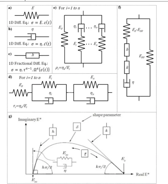
Figure 2-1. Bituminous materials seen in different length-scales: a) bituminous mixture cross-section, b) mastic schematic representation, c) bitumen scanning electron microscopy (SEM) image (Loeber et al. 1996), and d) schematic representation of bitumen and some of its components (Read et al. 2003). ... 9 Figure 2-2. Schematic representation of loading (strain, in figures a and b, or stress, in figures c and d) and response (stress or strain) (Di Benedetto and Corté 2005). ... 12 Figure 2-3. Schematic representation of different conceptual mechanical behaviour regions depending on the applied strain levels (ε) and the material temperature (T) for bitumen (Olard et al. 2005). Tg represents the glass transition temperature, where a brittle-to-ductile fracture behaviour is observed. ... 13 Figure 2-4. Schematic representation of different conceptual mechanical behaviour regions depending on the applied strain levels (ε) and the number of applied loading cycles (N) for bitumen (Mangiafico 2014). ... 13 Figure 2-5. Schematic representation of different conceptual mechanical behaviour regions depending on the applied strain levels (ε) and the number of applied loading cycles (N) for bituminous mixtures (Di Benedetto et al. 2013). ... 14 Figure 2-6. Linear viscoelasticity limits determined experimentally in bitumen and bituminous mixtures (Airey and Rahimzadeh 2004). ... 15 Figure 2-7. Schematic representation of different loading and response paths: different plots and time effect sensitivity. If curves I and II are always superimposed in the axes lij – rij (which correspond to stress-strain curve) and in the axes rij -rkl, the material is not sensitive to time effects (non viscous and non sensitive to ageing) in the considered loading domain (Di Benedetto et al. 2003)... 17 Figure 2-8. Schematic representation of the evolution of an intrinsic material property with

time, no evolution during ∆t meaning that the material is non-aging for that time span, possibly

being either time-independent or viscous (Di Benedetto et al. 2003). ... 18

Figure 2-9. Vertical modulus (Ev), at strain amplitude close to 10-5m/m, as a function of strain

rate (or equivalent strain rate for cyclic tests) for different geomaterials. The very important viscous sensitivity for bituminous mix is clearly visible (Di Benedetto et al. 2003). ... 19 Figure 2-10. Schematic representation of the time temperature superposition principle

application, using the time-shift factor aT (Di Benedetto et al. 2008). In the left-hand side, loading

and response signals are plotted as functions of the equivalent time (after time-shift). In the bottom right corner, the graph indicates that same values in the y-axis from the bottom left graph (response) are also plotted in the x-axis of the upper right graph. ... 20

(20)

Figure 2-11. Example of time-temperature superposition principle verification for linear viscoelasticity of bituminous mixture (Nguyen et al. 2013b). ... 22 Figure 2-12. Example of time-temperature superposition principle verification for the nonlinear domain (nonlinear viscoelasticity) of bituminous mixture (Nguyen et al. 2015). ... 23 Figure 2-13. Example of time-temperature superposition principle verification for the nonlinear domain (plastic deformations) of bituminous mixture (Nguyen et al. 2009). ... 24 Figure 2-14. Example of time-temperature superposition principle verification for crack propagation in bituminous mixture (Nguyen et al. 2013a). ... 25 Figure 2-15. Example of time-temperature superposition principle verification for the fatigue behaviour of bituminous mixture (Phan et al. 2017a). ... 26 Figure 2-16. Mechanical analogues - a) spring, b) dashpot, c) parabolic element, d) GKV, e) GMW, f) 2S2P1D – and g) 2S2P1D model interpretation in Cole-Cole plot (Specht et al. 2017).. 36 Figure 2-17. Example of coincidence of various normalised complex modulus curves from linear viscoelastic characterisation of different bituminous materials containing the same base bitumen (Pham et al. 2015a). Nine materials, differing with respect to the manufacturing process, fabrication temperature, the percentage of Recycled Asphalt Pavement (RAP), the use of additives and the air void content. ... 37 Figure 2-18. Schematic representation of the SHStS transformation (Mangiafico 2014)... 38 Figure 2-19. Example of bituminous mixture prediction using the SHStS transformation and bitumen linear viscoelastic characterisation from two different experimental procedures (using the Dynamic Shear Rheometer and using the Métravib) (Mangiafico 2014). ... 39 Figure 2-20. Example of bituminous mixture fatigue test experimental data (Tapsoba 2011): norm of complex modulus and phase angle (above), and measured surface temperature (below). . 43 Figure 2-21. Relationship between loading amplitude and number of cycles at fatigue (fatigue life) (Di Benedetto and Corté 2005). The figure presents schematically two different approaches: fitting Wöhler curve to describe this dependence, or searching for a “endurance limit” (Carpenter et al. 2003), which is the loading amplitude below which an infinite fatigue life would be expected. ... 46

Figure 2-22. Schematic representation of breakdown and build-up of thixotropic structure (Barnes 1997). Among possible explanation for shear-thinning and thixotropic behaviour are: alignment of elongated particles in the flow direction, loss of junctions in polymer solutions, rearrangement of microstructure in suspension and emulsion, and breakdown of flocs. ... 47 Figure 2-23. Equilibrium values of shear stress during “step” constant shear experiments, where the applied shear rate is changed in different loading blocks (Barnes 1997). ... 48

(21)

Figure 2-24. Verification of time temperature superposition for thixotropy (Nguyen 2011): norm of complex modulus variation (above), and phase angle variation (below). ... 49 Figure 2-25. Schematic representation of the contributions of the different physical phenomena (nonlinearity, heating, thixotropy and damage) on the measured norm of complex modulus during a cyclic loading test (at strain amplitude ε01) including rest (Nguyen 2011). ... 51 Figure 2-26. Directions of different phenomena on Black space (Nguyen 2011): example of experimental results (above), and schematic representation of the directions of the variation in complex (below). ... 52 Figure 2-27. Example of experimental results from tests on bituminous mixture consisting in the application of 100,000 cycles at 100μm/m followed by 24h of rest (Mangiafico 2014). Variations in norm of complex modulus (figure a) and phase angle (figure b) corresponding to different physical phenomena are represented: nonlinearity, heating, thixotropy and damage (called “unrecovered” in the figure, since an asymptotic value had not yet been obtained). ... 53 Figure 3-1. (a) ASR tests on bitumen and mastic hollow cylinder specimens mounted on a

MTS® hydraulic press testing frame, and (b) T-C tests on bituminous mixture cylindrical

specimens mounted on an Instron® hydraulic press testing frame. ... 57

Figure 3-2. Focus on the ASR test apparatus in the MTS® press (from Figure 3-1a), and details

on the test specimen with mounted sensors ... 58

Figure 3-3. Focus on the T-C test apparatus in the Instron® press (from Figure 3-1b), and

details on the test specimen with mounted sensors. ... 60 Figure 3-4. ASR specimen deformation during tests and interpretation of the applied shear strain. ... 61 Figure 3-5. Example of sinusoidal signals fitting in order to obtain amplitude and phase for experimental signals (sequence of two cycles for the stress, the radial strain, and the three axial strain measurements during a T-C test – example from nonlinearity investigation, Chapter 4). ... 65 Figure 3-6. Error on shear modulus introduced by the eccentricity between the external and the internal mould during ASR tests. a) Definition of studied eccentricity. b) Illustration of the specimen having a certain eccentricity, and its Finite Elements mesh (example with 3mm eccentricity). c) Mean error in shear modulus obtained with an eccentric specimen for different values of eccentricity. d) Zoom for eccentricities between 0 and 3mm. ... 67 Figure 3-7. Error on shear modulus introduced by a material loss due to flow under gravity. a) Definition of studied material loss (Mat_loss in %). b) Illustration of the specimen having a circular meniscus (diameter equals specimen thickness) due to material loss and its Finite Elements mesh (example with 0.01m Mat_loss). c) Mean error in shear modulus obtained with a specimen after a certain material loss. d) Zoom for material loss between 0 and 25%. ... 68 Figure 3-8. Bitumen ASR specimen preparation process. a) Clean mould before specimen preparation. b) Mould prepared for pouring with its protective adhesive tape. c) Mould with a

(22)

poured specimen (material is poured in excess in order to compensate for thermal expansion/contraction). d) Finished specimen. ... 70 Figure 3-9. Apparatus for mastic preparation ... 71 Figure 4-1. Scheme of the bituminous mixture complex modulus test (T-C setup, cf. Figure 3-3) loading path. ... 81 Figure 4-2. 2S2P1D model and WLF equation fitting of experimental data (BM1_A and BM1_C specimens) obtained from Tension/Compression (T-C) complex modulus tests at 50μm/m: a) Cole-Cole plot; b) Black diagram; c) normalized complex modulus master curve (at 15C); e) norm and f) phase angle of complex modulus; g) norm and h) phase angle of complex Poisson’s ratio master curve (at 15°C) with details on tested temperatures. ... 82 Figure 4-3. Detailed scheme of the 16 Strain Amplitude Sweep Tests for NonLinearity Evaluation (SASTENOLE) applied on BM1_B, with an example of results obtained for the norms of complex modulus and Poisson’s ratio during the eight sequences of the SASTENOLE test #13, at 14°C, 0.3Hz. A total of 128 sequences were performed and analysed on BM1_B. ... 85 Figure 4-4. Results obtained from SASTENOLE tests at 8°C, 10Hz (a, b, c) and 14°C, 0.3Hz

(d, e, f), for maximum targeted strain amplitude of 110μm/m: norm of complex modulus |E*_{| (top),}

phase angle φ (middle) and dissipated energy per cycle WN (bottom) are plotted as functions of

strain amplitude. ... 87

Figure 4-5. Norm of the complex modulus |E*| (a, top) and phase angle φ (b, bottom) obtained

from the SASTENOLE test at 14°C, 0.3Hz, for the four increasing strain amplitude loading paths:

sE and pφ are the slopes of the nonlinearity envelopes of, respectively, |E*| and φ. ... 90

Figure 4-6. Norm of the complex modulus |E*| (a, top) and phase angle φ (b, bottom) obtained

from the SASTENOLE test at 14°C, 0.3Hz, for decreasing strain amplitude loading paths: R2

values are calculated for the regressions of the initial points with lines of, respectively, sE and pφ

slopes (as calculated in Figure 4-5 for increasing strain amplitude loading paths). ... 91 Figure 4-7. Linear regression of pE values as a function of corresponding pφ values obtained

from all SASTENOLE tests on BM1_B at different temperatures and frequencies, for increasing strain amplitude loading paths (Figure 4-5). ... 93 Figure 4-8. Schemes of nonlinearity directions in Black (top) and Cole-Cole (bottom) spaces (cf. Eq. 4-6 and Eq. 4-8). ... 95 Figure 4-9. Results obtained from all SASTENOLE tests on BM1_B (scheme on Figure 4-3) at different temperatures and frequencies, for both decreasing and increasing strain amplitude loading paths, in Cole-Cole space: zooms are provided for data obtained at 14°C, 0.3Hz (bottom, left) and 8°C, 10Hz (bottom, right). For each combination of temperature and frequency, the regression was performed by combining data from both decreasing and increasing strain amplitude sweeps. ... 97 Figure 4-10. Results obtained from all SASTENOLE tests on BM1_B (scheme on Figure 4-3) at different temperatures and frequencies, for both decreasing and increasing strain amplitude

(23)

loading paths, in Black space: zooms are provided for data obtained at 8°C, 10Hz (bottom, left) and 14°C, 0.3Hz (bottom, right). For each combination of temperature and frequency, the regression was performed by combining data from both decreasing and increasing strain amplitude sweeps. ... 98 Figure 4-11. Results obtained from all SASTENOLE tests on BM1_B at different temperatures and frequencies, for both decreasing and increasing strain amplitude loading paths, in normalized Black space. ... 101 Figure 4-12. Comparison between the test conditions range for the first experimental campaign on bituminous mixture nonlinearity (BM1_B, cf. Figure 4-3) and for the second experimental campaign (on BM1_C). Including all testing sequences (increasing and decreasing sweeps at three different maximum targeted strain amplitudes) a total of 162 sequences were performed and analysed on BM1_C. ... 102 Figure 4-13. Results obtained from all SASTENOLE tests on BM1_C at different temperatures and frequencies, for both decreasing and increasing strain amplitude loading paths, in (a) Cole-Cole plot (comparable to Figure 4-9 for BM1_B), (b) Black space (comparable to Figure 4-10 for BM1_B), and (c) normalized black space (comparable to Figure 4-11 for BM1_B). ... 103

Figure 4-14. pE and pφ results obtained from all SASTENOLE tests on BM1_C (BM1_B

results on Figure 4-7 also represented here) at different temperatures and frequencies, for

increasing strain amplitude loading paths: a) pE as a function of corresponding pφ; b) pE (intensity

of nonlinearity effect) as a function of corresponding pE/pφ (which gives nonlinearity direction); c)

isotherms for pE; and d) pE master curve, d) pE/pφ master curve, and f) pφ master curve, all

constructed using WLF parameters from LVE characterisation (Table 4-1). The master curves are presented at 15°C. ... 105

Figure 4-15. LVE limit (in terms of axial strain amplitude,

ε

0.95%, figs. a and b, and axial stress

amplitude,

σ

0.95%, figs. c and d) obtained from SASTENOLE results (cf. |pE·ε0| ≤ 0.05 results in

Table 4-7) on bitumen BM1_C as a function of norm of complex modulus (figs. a and c) and time-shifted frequency (figs b and d)... 107

Figure 4-16. Norm and phase angle of complex modulus (|E*|, φ, figures a and b) and of

Poisson’s ratio (|ν*|, φν, figures c and d) obtained during increasing and decreasing strain sweeps of

SASTENOLE test for maximum targeted strain amplitude of 110μm/m at -4°C, 1Hz. ... 110

Figure 4-17. Norm and phase angle of complex modulus (|E*|, φ, figures a and b) and of

Poisson’s ratio (|ν*_{|, φ}

ν, figures c and d) obtained during increasing and decreasing strain sweeps of

SASTENOLE test for maximum targeted strain amplitude of 110μm/m at 28°C, 0.1Hz. ... 111

Figure 4-18. Norm |ν*| (top) and phase angle φν of Poisson’s ratio (bottom) obtained from

SASTENOLE test at -4°C, 1Hz, for the three increasing strain amplitude (figures a and b) and for

the three decreasing strain amplitude loading paths (figures c and d): sν and pφν are the slopes of

the nonlinearity envelopes of, respectively, |ν*_{| and φ}

(24)

Figure 4-19. Norm |ν*_{| (top) and phase angle φ}

ν of Poisson’s ratio (bottom) obtained from

SASTENOLE test at 28°C, 0.1Hz, for the three increasing strain amplitude (figures a and b) and

for the three decreasing strain amplitude loading paths (figures c and d): sν and pφν are the slopes of

the nonlinearity envelopes of, respectively, |ν*| and φν. ... 112

Figure 4-20. Example of results for the simulation of perfectly linear viscoelastic response of BM1_A (using KVG model parameters given in Table 4-9, and specimen diameter 75.3mm), including transient effects, to the SASTENOLE loading path (increasing and decreasing sweeps), obtained at 14°C and 0.3Hz with maximum strain amplitude of 100μm/m: a) Modulus from increasing and decreasing sweeps as a function of loading cycles; a) Modulus from increasing and decreasing sweeps as a function of the applied strain amplitude; and examples of hysteresis loop (including the actual response and the fitted sine functions used to obtain modulus) at c) the 2nd cycle and d) the 10th_{cycle. ... 115}

Figure 4-21. Scheme of the bitumen and mastic complex modulus test (ASR setup, cf. Figure 3-2, and Figure 3-4 for a deformation scheme) loading path. ... 116 Figure 4-22. 2S2P1D fitting of experimental data (BM1_A and BM1_C specimens) obtained from ASR complex shear modulus tests at low strain amplitude (force signal amplitude around 0.3kN): a) Cole-Cole plot; (b) Black diagram; c) normalized complex modulus master curve (at 15°C); d) norm of complex modulus, and e) phase angle master curves (at 15°C) with details on tested temperatures; and f) comparison of norm of axial complex modulus master curves (at 15°C) for the three studied materials. ... 117 Figure 4-23. Detailed scheme of the Strain Amplitude Sweep (SAS) tests conducted using the ASR, with an example of results for B5070 at 11.1°C, presenting the obtained norm of complex shear modulus and the in-specimen temperature during the loading sequences at 3Hz. ... 119 Figure 4-24. Maximum temperature increase during SAS tests on bitumen and mastic (at the last cycle of loading at a given frequency and strain amplitude, cf. Figure 4-23). The figure presents the temperature increase for tests on bitumen at 11.1°C and all frequencies (figure a), on mastic at 11.1°C and all frequencies (figure b), on bitumen and mastic at 10Hz and all temperatures (figure c) and a zoom on these last results (figure d). ... 120 Figure 4-25. Example of a set of experimental results (norm and phase angle of complex shear modulus) for SAS tests using the ASR (tests at 6.3°C on mastic M5070_30pc40-70), with details on the method for determination of the asymptotic “linear” values (at 0μm/m) and of the LVE limit in terms of strain amplitude. ... 122 Figure 4-26. SAS experimental results in normalized Black curves (normalized equivalent complex modulus as a function of the normalized phase angle) for all tested temperatures and frequencies on bitumen B5070 and mastic M5070_30pc40-70. ... 123 Figure 4-27. SAS experimental results at 0.1Hz for all tested temperatures in normalized Black curves (normalized equivalent complex modulus as a function of the normalized phase angle) for bitumen B5070 and mastic M5070_30pc40-70. ... 124

(25)

Figure 4-28. pE/pφ results obtained from all SAS tests on B5070 and on M5070_30pc40-70 at

different temperatures and frequencies: a) pE/pφ as a function of frequency; b) pE/pφ master curves,

constructed using WLF parameters from LVE characterisation (Table 4-10); c) pE/pφ master curves

including BM1_C results (cf. Figure 4-14). The master curves are presented at 15°C. ... 125

Figure 4-29. LVE limit (in terms of shear strain amplitude,

γ

0.95%, figs. a, b, e, and f, and shear

stress amplitude,

τ

0.95%, figs. c, d, and g) obtained from SAS test results (cf. example in Figure 4-25) on bitumen B5070 and mastic M5070_30pc40-70 as a function of norm of complex shear modulus (a through e) and time-shifted frequency at 15°C (f and g). ... 126 Figure 4-30. Comparison of the determined LVE limits (in terms of axial or shear strain amplitude,

ε

0.95% or

γ

0.95%, figure a, and axial or shear stress amplitude,

σ

0.95% or

τ

0.95%, figure b) obtained from SASTENOLE and SAS test results (cf. Figure 4-15 and Figure 4-29) on bitumen B5070, mastic M5070_30pc40-70 and BM1_C as a function of norm of complex shear modulus. ... 127

Figure 4-31. Comparison of the determined LVE limits (in terms of axial or shear strain amplitude,

ε

0.95% or

γ

0.95%, figure a, and axial or shear stress amplitude,

σ

0.95% or

τ

0.95%, figure b) obtained from SASTENOLE and SAS test results (cf. Figure 4-15 and Figure 4-29) on bitumen B5070, mastic M5070_30pc40-70 and BM1_C as a function of the time-shifted frequency (with the same WLF parameters as for linear characterisation, cf. Table 4-1 and Table 4-10). The results are presented as master curves at 15°C. ... 129 Figure 5-1. Scheme for the proposed thermomechanical calculations. ... 135 Figure 5-2. Loading scheme (Nguyen 2011) of a Phase I Fatigue test (example of tests on BM2_A). ... 137 Figure 5-3. a) Considered idealized heterogeneous bituminous mixture (monodisperse spherical particles in a mastic phase) and b) Zoom on the elementary cell called “Elementary Heterogeneous Volume” (EHeV) used for 3D heterogeneous calculation. ... 138 Figure 5-4. Aggregate gradation of the two studied materials: in mass (left axis, classical representation without bitumen) and in volume (right axis, considering air voids and bitumen).. 138 Figure 5-5. Scheme of the steps necessary to the simplified thermomechanical calculations. 139 Figure 5-6. Schematic definition of the normalized parameter (M) giving the influence of temperature on |E*| for a given loading frequency. ... 141 Figure 5-7. Explanation of strain calculation from displacement δ (applied load F in tension-compression): a) Case of the Elementary Homogeneous Volume (EHoV) and b) Case of the Elementary Heterogeneous Volume (EHeV) ... 143 Figure 5-8. 3D heterogeneous calculation results with e/R = 0.015 (fixed parameters corresponding to the studied bituminous mixture, tested at 12.3°C and 3Hz for a strain amplitude of 116μm/m, cf. also test results in Figure 5-10 and Figure 5-11): (above) strain amplitude and

(26)

cumulated force on a disc of radius r and (below) temperature increase per cycle for local adiabatic conditions (i.e. no heat transfer) as a function of relative position (r/R) ... 146 Figure 5-9. Modulus (left axis) and relative modulus (right axis) decrease per cycle as a function of e/R (fixed parameters correspond to BM3 and tested at 12.3°C and 3Hz for a strain amplitude of around 116μm/m, see also test results Figure 5-10) ... 147 Figure 5-10. Initial decrease of norm of complex modulus for BM3_A, tested at 12.3°C and 3Hz for a strain amplitude of 116μm/m (cf. also test results in Figure 5-11): data and prediction considering the 3 considered calculations: i) homogeneous heat in the mix, ii) Homogeneous heat in bituminous phase and iii) 3D heterogeneous thermomechanical calculation. Up to 10,000 cycles (b) and, zoom up to 100 cycles (a). ... 149 Figure 5-11. For BM2, modelled (3D heterogeneous thermomechanical calculation, cf. Section

5.5.3 and Figure 5-10a) normalized initial modulus decrease (-d|E bm* |/dN)/|Ebm*|) as a function of

the results obtained from experiments (for cycles between 5 and 7s of loading) at different temperatures and frequencies with different strain amplitudes (10 tests): a) labelled by frequencies, and b) labelled by temperatures. ... 153 Figure 5-12. For BM3, modelled (3D heterogeneous thermomechanical calculation, cf. Section

5.5.3 and Figure 5-10a) normalized initial modulus decrease (-d|E bm* |/dN)/|Ebm*|) as a function of

the results obtained from experiments (for cycles between 5 and 7s of loading) at different temperatures and frequencies with different strain amplitudes (13 tests): a) labelled by frequencies, and b) labelled by temperatures. ... 153 Figure 5-13. Investigation of relationships of the time for correspondence between calculated and experimental slopes of norm of complex modulus observed for Phase I Fatigue tests. Example on BM3. a) Time correspondence (beginning and end of correspondence) for the calculation considering homogeneous heat in bitumen as a function of the time-shifted frequency. b) Number of cycles for the beginning of correspondence for the calculation considering homogeneous heat in bitumen and homogeneous heat in mixture as a function of the number of cycles for the beginning of correspondence for the calculation considering heterogeneous heat in mastic. c) A normalised parameter (involving correspondence time, strain amplitude, and complex modulus) as a function of the time-shifted frequency. ... 156 Figure 5-14. Flowchart describing performed FEM calculations: thermal analysis and mechanical analysis. ... 158 Figure 5-15. a) Idealized heterogeneous bituminous mixture; b) Zoom on the meshed elementary cell called “Elementary Heterogeneous Volume” (EHeV) used for 3D FEM analysis; c) considerations for FEM thermal analysis; d) considerations for FEM mechanical analysis. .... 160 Figure 5-16. Temperature distribution and bituminous mixture relative modulus change at a) 0.1s; b) 1s; and c) 10s for e = 3μm and sinusoidal loading at 10Hz and 150μm/m strain amplitude applied on the bituminous mixture (the model represents BM3). ... 161

(27)

Figure 5-17. Results for the first 100 cycles of sinusoidal loading for e = 3µm. a) Modulus and temperature changes calculated with a “linearized” heat production during each cycle; and b) and c) zoom for cycles #99 and #100 including the temperature change considering “real” heat production at points A (maximum temperature change) and B (minimum temperature change). . 162 Figure 6-1. Scheme of the Alternating Strain Amplitude test loading path, including details on the applied strain amplitudes during loading (no rest periods are applied). ... 169 Figure 6-2. Scheme of Load and Rest Periods tests loading path, including representation of the applied strain amplitudes during loading and of the applied small strain amplitudes during rest. 170 Figure 6-3. 2S2P1D model (cf. Chapter 4, Figure 4-22 and Table 4-10) for bitumen (B5070) and mastic (M5070_30pc40-70), with indications of complex modulus obtained at 10Hz at various temperatures from 10 to 21°C: Representation on a) Cole-Cole plot and b) Black diagram (with arithmetic scale for the norm of complex modulus). ... 172 Figure 6-4. Alternating Strain Amplitudes (ASA) test results for bitumen (B5070_G): a) Norm of complex modulus, b) phase angle, c) mean in-specimen temperature, and d) shear strain amplitude as a function of time, for a test performed at constant frequency of 10Hz (1s = 10cycles)... 176 Figure 6-5. Alternating Strain Amplitudes (ASA) test results for bitumen (B5070_G) represented in Black space (natural non-log axis for norm of complex modulus as a function of the phase angle. ... 177 Figure 6-6. Experimental results (B5070_D) for LRP tests: 5 LRP loops with 10,000 cycles and 4h rest on bitumen submitted to 20,000μm/m sinusoidal loading: a) Norm of complex modulus and phase angle as a function of time, and b) shear strain amplitude and temperature as a function of time. ... 181 Figure 6-7. Experimental results (B5070_D) for LRP tests: 5 LRP 20,000μm/m sinusoidal loading loops with 10,000 cycles each on bitumen: a) Norm of complex shear modulus, b) phase angle, c) mean in-specimen temperature, and d) dissipated energy per cycle as a function of the number of applied cycles... 182 Figure 6-8. Experimental results (B5070_D) for LRP tests: 5 LRP 20,000μm/m sinusoidal loading loops with 10,000 cycles each on bitumen: representation on a) Black space, and b) Cole-Cole diagram. ... 183

Figure 6-9. Experimental results (B5070_D) for LRP tests: 5 LRP 20,000μm/m sinusoidal loading loops with 10,000 cycles each on bitumen: a) Normalised (the initial modulus being

considered as the result at the 3rd cycle) norm of complex shear modulus, and b) normalised phase

angle as a function of number of applied cycles; and c) representation of the results on a normalised Black space. ... 184 Figure 6-10. Experimental results for LRP tests: analysis of the unrecovered relative change in complex modulus after 4h rest: a) bitumen (B5070_C) with 3,600μm/m sinusoidal loading, b)

(28)

bitumen (B5070_A) with 10,000μm/m, c) bitumen (B5070_B and B5070_D) with 20,000μm/m, d) mastic (M5070_30pc40-70_C) with 1,000μm/m, e) mastic (M5070_30pc40-70_A) with 3,300μm/m, and f) mastic (M5070_30pc40-70_B) with 8,800μm/m. ... 186 Figure 6-11. Slopes of the unrecovered change in norm of complex modulus obtained from LRP tests on bitumen and mastic as a function of the applied shear strain amplitude. ... 187 Figure 6-12. Scheme of the utilised correction for the temperature effect (T-effect) on the complex modulus, with an example for bitumen (the hypothesis for correction is the same for mastic). The correction uses as input parameters the 2S2P1D complex moduli (G*2S2P1D, fitted for low strain amplitudes) at the initial (Tini) and the current (T) measured temperatures, and the measured complex modulus (G*) during the LRP test (performed at higher strain amplitudes). a) Complex modulus at different temperatures on a Black diagram (cf. Figure 4-22 and Table 4-10 and Figure 6-3). b) Temperature effect on the calculated 2S2P1D complex modulus (low strain amplitude,

γ

0,1) and indication of nonlinearity effect on . c) Scheme of the temperature effect on

the measured complex modulus (at higher strain amplitude,

γ

0,2), after the effect of nonlinearity is

obtained (cf. Chapter 4). ... 189 Figure 6-13. Temperature evolution as a function of the number of applied cycles during the first loading loop of LRP test on bitumen specimen B5070_D. Three temperature evolution curves are presented: measured mean in-specimen temperature, necessary temperature to explain phase angle variation during loading, and necessary temperature to explain modulus variation during loading. ... 190 Figure 6-14. Experimental results (B5070_D) for LRP tests (5 LRP tests with 10,000 cycles of 20,000μm/m sinusoidal loading and 4h rest loops on bitumen): a) Black diagram representation of the results including details of the number of cycles during loading and the time of rest during rest periods, and a representation of the nonlinearity effect; b) results after temperature correction. The figure present also a 2S2P1D model prediction, with indication of LVE complex modulus at 10Hz and three temperatures, 11.1°C (Tini), 15°C and 19°C. ... 193 Figure 6-15. Experimental results (B5070_D) for LRP tests (5 LRP tests with 10,000 cycles of 20,000μm/m sinusoidal loading and 4h rest loops on bitumen): Black diagram representation of a) the raw experimental results and the results after the temperature correction and b) the experimental results after temperature and damage correction. The figure present also a 2S2P1D model prediction, with indication of LVE complex modulus at 10Hz and three temperatures, 11.1°C (Tini), 15°C and 19°C. ... 195 Figure 6-16. Experimental results (B5070_E) for LRP tests: 5 LRP loops with 20,000 cycles and 14h rest on bitumen submitted to 20,000μm/m sinusoidal loading. a) Norm of complex modulus and phase angle as a function of time, and b) shear strain amplitude and temperature as a function of time. ... 198 Figure 6-17. Comparison (in Black space) of LRP test results with different test parameters: LRP test with 10,000 cycles of sinusoidal loading at 20,000μm/m and 4h rest loops and 20,000

(29)

cycles of sinusoidal loading at 20,000μm/m and 14h rest loops on bitumen (B5070_E) at 11.0°C and 10Hz. ... 199 Figure 6-18. Experimental results (B5070_D) for the fatigue test performed immediately after the last rest loop of the LRP test (cf. Figure 6-6) with to 20,000μm/m sinusoidal loading and determination of the number of cycles at failure (Nf). a) Norm of complex modulus and phase angle as a function of the number of applied cycles, and b) shear strain amplitude and temperature as a function of the number of applied cycles. ... 201 Figure 6-19. Experimental results from the fatigue tests performed immediately after the last rest loop of the LRP tests: number of cycles at failure (Nf), defined considering changes in trend on the rate of change in modulus and on the phase angle, as a function of the shear strain amplitude (Whöler curves). a) Results considering only cycles from the fatigue test, and b) results considering both the cycles from the LRP and the cycles from the fatigue test (the effect of all cycles on the fatigue damage is considered to cumulate). ... 202 Figure B-1. Set of experimental results (norm and phase angle of complex shear modulus) for SAS tests using the ASR (tests at 6.3°C on bitumen B5070), with details on the method for determination of the asymptotic “linear” values (at 0μm/m) and of the LVE limit in terms of strain amplitude. ... 255 Figure B-2. Set of experimental results (norm and phase angle of complex shear modulus) for SAS tests using the ASR (tests at 11.1°C on bitumen B5070), with details on the method for determination of the asymptotic “linear” values (at 0μm/m) and of the LVE limit in terms of strain amplitude. ... 256 Figure B-3. Set of experimental results (norm and phase angle of complex shear modulus) for SAS tests using the ASR (tests at -3.2°C on mastic M5070_30pc40-70), with details on the method for determination of the asymptotic “linear” values (at 0μm/m) and of the LVE limit in terms of strain amplitude. ... 257 Figure B-4. Set of experimental results (norm and phase angle of complex shear modulus) for SAS tests using the ASR (tests at 6.3°C on mastic M5070_30pc40-70), with details on the method for determination of the asymptotic “linear” values (at 0μm/m) and of the LVE limit in terms of strain amplitude. ... 258 Figure B-5. Set of experimental results (norm and phase angle of complex shear modulus) for SAS tests using the ASR (tests at 11.1°C on mastic M5070_30pc40-70), with details on the method for determination of the asymptotic “linear” values (at 0μm/m) and of the LVE limit in terms of strain amplitude. ... 259 Figure B-6. Set of experimental results (norm and phase angle of complex shear modulus) for SAS tests using the ASR (tests at 15.0°C on mastic M5070_30pc40-70), with details on the method for determination of the asymptotic “linear” values (at 0μm/m) and of the LVE limit in terms of strain amplitude. ... 260

(30)

Figure C-1. Experimental results (B5070_C) for LRP tests: 5 LRP loops with 10,000 cycles and 4h rest on bitumen submitted to 3,600μm/m sinusoidal loading: a) Norm of complex modulus and phase angle as a function of time, and b) shear strain amplitude and temperature as a function of time. ... 262 Figure C-2. Experimental results (B5070_C) for LRP tests: 5 LRP 3,600μm/m sinusoidal loading loops with 10,000 cycles each on bitumen: a) Norm of complex shear modulus, b) phase angle, c) mean in-specimen temperature, and d) dissipated energy per cycle as a function of the number of applied cycles... 263 Figure C-3. Experimental results (B5070_C) for LRP tests: 5 LRP 3,600μm/m sinusoidal loading loops with 10,000 cycles each on bitumen: representation on a) Black space, and b) Cole-Cole diagram. ... 264

Figure C-4. Experimental results (B5070_C) for LRP tests: 5 LRP 3,600μm/m sinusoidal loading loops with 10,000 cycles each on bitumen: a) Normalised (the initial modulus being

considered as the result at the 3rd cycle) norm of complex shear modulus, and b) normalised phase

angle as a function of number of applied cycles; and c) representation of the results on a normalised Black space. ... 265 Figure C-5. Experimental results (B5070_C) for LRP tests (5 LRP tests with 10,000 cycles of 3,600μm/m sinusoidal loading and 4h rest loops on bitumen): a) Black diagram representation of the results including details of the number of cycles during loading and the time of rest during rest periods, and a representation of the nonlinearity effect; b) results after temperature correction. The figure present also a 2S2P1D model prediction, with indication of LVE complex modulus at 10Hz and three temperatures, 11.1°C (Tini), 11.4°C and 11.7°C. ... 266 Figure C-6. Experimental results (B5070_C) for LRP tests (5 LRP tests with 10,000 cycles of 3,600μm/m sinusoidal loading and 4h rest loops on bitumen): Black diagram representation of a) the raw experimental results and the results after the temperature correction and b) the experimental results after temperature and damage correction. The figure present also a 2S2P1D model prediction, with indication of LVE complex modulus at 10Hz and three temperatures, 11.1°C (Tini), 11.4°C and 11.7°C. ... 267 Figure C-7. Experimental results (B5070_A) for LRP tests: 5 LRP loops with 10,000 cycles and 4h rest on bitumen submitted to 10,000μm/m sinusoidal loading: a) Norm of complex modulus and phase angle as a function of time, and b) shear strain amplitude and temperature as a function of time. ... 268 Figure C-8. Experimental results (B5070_A) for LRP tests: 5 LRP 10,000μm/m sinusoidal loading loops with 10,000 cycles each on bitumen: a) Norm of complex shear modulus, b) phase angle, c) mean in-specimen temperature, and d) dissipated energy per cycle as a function of the number of applied cycles... 269 Figure C-9. Experimental results (B5070_A) for LRP tests: 5 LRP 10,000μm/m sinusoidal loading loops with 10,000 cycles each on bitumen: representation on a) Black space, and b) Cole-Cole diagram. ... 270