Supplement of

Supplement of Biogeosciences, 13, 6651–6667, 2016

http://www.biogeosciences.net/13/6651/2016/

doi:10.5194/bg-13-6651-2016-supplement

© Author(s) 2016. CC Attribution 3.0 License.

Supplement of

Challenges in modelling isoprene and monoterpene emission dynamics of

Arctic plants: a case study from a subarctic tundra heath

Jing Tang et al.

Correspondence to:

Jing Tang (jing.tang@bio.ku.dk)

1

Supplementary material

S1 PFTs simulated for the study area

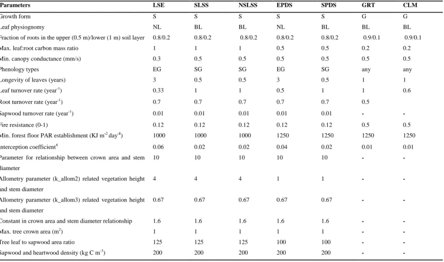
Table S1 Detailed descriptions of the PFT parameters for the study area (Abisko, tundra heath). LSE: low shrubs evergreen; SLSS: Salix, low shrubs summergreen; NSLSS: non-Salix, low shrubs summergreen; EPDS: evergreen prostrate dwarf shrubs; SPDS: summergreen prostrate dwarf shrubs;

5

GRT: graminoid tundra; CLM: cushion forbs, lichens and mosses tundra; S: shrub; G: grass; NL: needleleaf; BL: broadleaf; Max.: maximum; Min.: minimum; EG: evergreen; SG: summergreen; GDD5: growing degree days above 5 ο

C; GDD0: growing degree days above 0 oC.

Parameters LSE SLSS NSLSS EPDS SPDS GRT CLM

Growth form S S S S S G G

Leaf physiognomy NL BL BL NL BL BL BL

Fraction of roots in the upper (0.5 m)/lower (1 m) soil layer 0.8/0.2 0.8/0.2 0.8/0.2 0.8/0.2 0.8/0.2 0.9/0.1 0.9/0.1 Max. leaf:root carbon mass ratio 1 1 1 0.5 0.5 0.2 0.2 Min. canopy conductance (mm/s) 0.3 0.5 0.5 0.5 0.5 0.5 0.5

Phenology types EG SG SG EG SG any any

Longevity of leaves (years) 3 0.5 0.5 3 0.5 1 1 Leaf turnover rate (year-1_{) 0.33 1 1 0.5 1 1 0.6}

Root turnover rate (year-1_{) 0.7 0.7 0.7 0.7 0.7 0.5}

Sapwood turnover rate (year-1_{) 0.01 0.01 0.01 0.01 0.01}

- -

Fire resistance (0-1) 0.12 0.12 0.12 0.12 0.12 0.5 0.5 Min. forest floor PAR establishment (KJ m-2 day-1) 1000 1000 1000 1250 1250 1250 1250 Interception coefficient€ _{0.06 0.02 0.02 0.04 0.02 0.01 0.01}

Parameter for relationship between crown area and stem diameter

10 10 10 10 10 - -

Allometry parameter (k_allom2) related vegetation height and stem diameter

4 4 4 1 1 - -

Allometry parameter (k_allom3) related vegetation height and stem diameter

0.67 0.67 0.67 0.67 0.67 - -

Constant in crown area and stem diameter relationship 1.6 1.6 1.6 1.6 1.6 - -

Max. tree crown area (m2) 1 1 1 1 1 - -

Tree leaf to sapwood area ratio 125 125 125 100 100 - -

Growth efficiency threshold (kg C m-2 _{leaf yr}-1_{) 0.012 0.012 0.012 0.01 0.01 - -}

Max. establishment rate (samplings m-2 _yr-1₎* _{0.6 0.8 1 0.8 0.8 - -}

Recruitment shape parameterГ 10 10 7 10 10 - -

Mean non-stress longevity (yr) 25 25 25 30 30 - -

GDD5 required to obtain full leave cover 0 50 50 0 50 50 1 Photosynthesis min. temperature (o_{C) -4 -4 -4 -4 -4 -4 -4}

Approximate lower range of temperature optimum for photosynthesis

10 10 10 10 10 10 10

Approximate upper range of temperature optimum for photosynthesis

30 30 30 25 25 25 25

Photosynthesis max temperature (o_{C) 38 38 38 38 38 38 38}

Min. temperature of coldest month for survival -32.5 -40 -40 -1000 -1000 -1000 -1000 Min. temperature of coldest month for establishment -32.5 -32.5 -32.5 -1000 -1000 -1000 -1000 Max. temperature of coldest month for establishment 1000 1000 1000 1000 1000 1000 1000 Min. temperature of warmest month for establishment -1000 -1000 -1000 -1000 -1000 -1000 -1000 Min. GDD5 for establishment 100 100 100 0 0 0 0 Min. GDD0 for reproduction 300 300 300 150 150 150 50 Max. GDD0 for reproductionξ - - - 1500 - 1400 -

Min. snow cover (mm) - - - 20 20 - 50

Maintenance respiration coefficient 1 1 1 1 1 1 1 Min. fraction of available soil water in upper soil layer

during growing season

0.1 0.1 0.1 0.01 0.01 0.01 0.01 Max. evapotranspiration rate 5 5 5 5 5 5 5 Litter moisture flammability threshold (fraction of

available water holding capacity)

0.3 0.3 0.3 0.3 0.3 0.2 Sapwood C:N mass ratio 330 330 330 330 330 - -

Fine root C:N mass ratio 29 29 29 29 29 29 29 Maximum nitrogen uptake per fine root (kg N kg C-1 _day-1_{) 0.0028 0.0028 0.0028 0.0028 0.0028 0.00551 0.00551}

Half-saturation concentration for N uptake (kg N l-1_{) 1.477E-06 1.477E-06 1.477E-06 1.477E-06 1.477E-06 1.886E-06 1.886E-06}

Fraction of sapwood or root for N long-term storage 0.3 0.3 0.3 0.3 0.3 0.3 0.3 Specific leaf area (m2 _{kg C}-1_{) 12.56 24.25 24.25 12.56 24.25 19.75 25.8}

Isoprene emission capacity (µg C g-1 _h-1_{) E}

IS20 1.751/1.737 11.305/11.213 2.512/2.492 1.411/1.400 14.117/14.0

03

9.898/9.818 1.198/1.188 Isoprene emissions show a seasonality (1) or not (0) 0 1 1 0 1 1 0

Monoterpene emission capacity (µg C g-1 _h-1_{) E}

3

Fraction of monoterpene production that go into storage pool

0.5 0.5 0.5 0.5 0.5 0.5 0 Aerodynamic conductance (m s-1) 0.04 0.04 0.04 0.03 0.03 0.03 0.03

*, ξ: the values were adjusted based on the point intercepted-based observations to increase/decrease relative abundance; €

: a dimensionless biome-dependent proxy for rainfall region (Gerten et al., 2004). Г

: relates to life history class of plant functional types. High values of this parameter represent a steeper decline in establishment rate as shading reduces potential seedling growth.

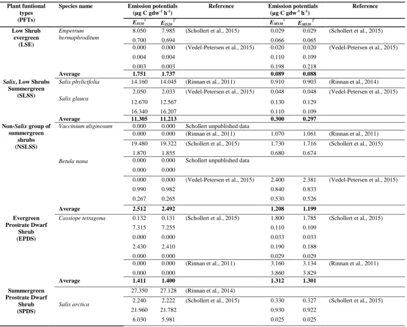
Table S2 Detailed description of literature values used for parameterizing PFT emission capacities, isoprene (IS, µg C gdw-1 h-1) and monoterpene (MS, µg C gdw-1 h-1) emissions at 20°C and 30°C. For some PFTs, the multiple data values from the same study are from different sampling dates in the original publications.

Plant funtional types (PFTs)

Species name Emission potentials (µg C gdw-1 _h-1₎

Reference Emission potentials (µg C gdw-1 _h-1₎ Reference EIS30† EIS20 Г _E MS30† EMS20 Г Low Shrub evergreen (LSE) Empetrum hermaphroditum

8.050 7.985 (Schollert et al., 2015) 0.029 0.029 (Schollert et al., 2015) 0.700 0.694 0.066 0.065

0.000 0.000 (Vedel-Petersen et al., 2015) 0.020 0.020 (Vedel-Petersen et al., 2015) 0.004 0.004 0.110 0.109

0.003 0.003 0.198 0.218

Average 1.751 1.737 0.089 0.088

Salix, Low Shrubs

Summergreen (SLSS)

Salix phylicifolia 14.160 14.045 (Rinnan et al., 2011) 0.910 0.903 (Rinnan et al., 2014)

Salix glauca

2.050 2.033 (Vedel-Petersen et al., 2015) 0.048 0.048 (Vedel-Petersen et al., 2015) 12.670 12.567 0.130 0.129 16.340 16.207 0.110 0.109 Average 11.305 11.213 0.300 0.297 Non-Salix group of summergreen shrubs (NSLSS)

Vaccinium uliginosum 0.000 0.000 Schollert unpublished data

Betula nana

0.000 0.000 (Rinnan et al., 2011) 1.070 1.061 (Rinnan et al., 2011) 19.480 19.322 (Schollert et al., 2015) 1.730 1.716 (Schollert et al., 2015)

1.870 1.855 0.680 0.674 0.000 0.000 Schollert unpublished data

0.000 0.000

0.000 0.000 (Vedel-Petersen et al., 2015) 2.400 2.381 (Vedel-Petersen et al., 2015) 0.990 0.982 0.840 0.833 0.267 0.265 0.530 0.526 Average 2.512 2.492 1.208 1.199 Evergreen Prostrate Dwarf Shrub (EPDS)

Cassiope tetragona 0.132 0.131 (Schollert et al., 2015) 1.800 1.785 (Schollert et al., 2015) 7.315 7.255 0.110 0.109

0.000 0.000 0.033 0.033 2.430 2.410 0.190 0.188 0.000 0.000 0.029 0.029

0.000 0.000 (Rinnan et al., 2011) 3.160 3.134 (Rinnan et al., 2011) 0.000 0.000 3.860 3.829 Average 1.411 1.400 1.312 1.301 Summergreen Prostrate Dwarf Shrub (SPDS) Salix arctica 27.350 27.128 (Rinnan et al., 2014)

2.240 2.222 (Schollert et al., 2015) 0.330 0.327 (Schollert et al., 2015) 21.960 21.782 0.930 0.922

5

4.640 4.602 (Vedel-Petersen et al., 2015) 0.430 0.427 (Vedel-Petersen et al., 2015) 13.260 13.152 0.720 0.714 23.340 23.151 1.700 1.686 Average 14.117 14.003 0.428 0.425 Graminoid (GRT) Eriophorum angustifolium

20.240 20.076 (Ekberg et al., 2009) 0.000 0.000 (Ekberg et al., 2009) 10.001 9.920 0.735 0.729 3.463 3.435 27.359 27.137 26.432 26.217 Carex rostrata 14.832 14.712 0.080 0.080 0.266 0.264 1.704 1.690 6.150 6.100 7.521 7.460 Average 9.898 9.818 0.000 0.000 Cushion forbs, lichens, and moss

tundra (CLM)

Sphagnum cuspidatum 1.160 1.151 Tiiva unpublished data

Sphagnum fuscum 0.864 0.857 (Hanson et al., 1999)

Sphagnum balticum 2.034 2.017

(Ekberg et al., 2011) 2.108 2.091

3.216 3.190 1.703 1.689

Warnstorfia exannulata 0.132 0.131 (Tiiva et al., 2007) 0.010 0.009 (Faubert et al., 2010)

Aulacomnium palustre 2.860 2.837 Tiiva unpublished data

Dicranum polysetum 0.043 0.043 (Hanson et al., 1999)

Hylocomium splendens 0.011 0.011

Ptilidium ciliare 0.024 0.024

Sphagnum* 0.220 0.218 (Janson and De Serves, 1998) 0.050 0.050 (Janson et al., 1999)

Average 1.198 1.188 0.030 0.029

*There is no species name in the original publication. †: These values from original publications were standardized to 30 °C using the Guenther’s

algorithm (Guenther et al., 1993);

6

S2 Sensitivity testing of α

A uniform sampling of the parameter α

(1000 times, under the range of 0.02 to 0.125 µmol CO

µmol photons

) was

implemented and the model simulations with different α

values were conducted to investigate how the modelled GPP, ER and

LAI are influenced by the parameter α

. Closed-chamber based CO

fluxes and point intercepted-based plant coverage in the

5

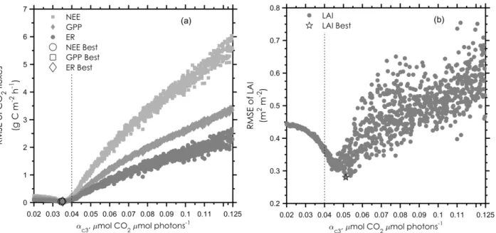
control plots were compared with the simulated outputs. Modelled GPP, ER, NEP and LAI were largely influenced by the

parameter value of α

(Fig. S1). The root mean square error (RMSE) values of the four investigated variables showed a slight

decrease, followed by a sharp increase with increasing α

. For the RMSE of GPP, ER and NEP, the first quantile occurs at the

lowest value range of α

, with the RMSE of LAI spreading between 0.03 and 0.07. The parameter values with the lowest RMSE

(Best) for GPP, ER, LAI are 0.034, 0.037 and 0.051 µmol CO

µmol photons

, respectively.

10

Figure S1 The root mean square error (RMSE) of the modelled net ecosystem production (NEP), gross primary production (GPP), ecosystem respiration (ER), (a) and leaf area index (LAI), (b) related to the observations for the years 2006 and 2007. The parameter values with the lowest RMSE (Best, in the legend) are marked. The dashed lines point out the αc3 selected for this study.

7

S3 Seasonal variation of BVOC emissions

The span of the BVOC measurements covered the main growing seasons over three years. The modelled daily average emission

rates in the C plots showed pronounced day-to-day and seasonal variations (Fig. S2). The modelled emissions of isoprene and

monoterpenes were low in Spring and Autumn, and peaked on warm days during the Summer. The day-to-day variations in the

emissions agreed well with the variations of T and PAR. When both T and PAR were high, the peaks of both isoprene and

5

monoterpene emissions occurred. The observed magnitude of isoprene emissions during daytime showed large spatial variation

between the blocks for the days with the observed high average emission rates (blue error bars in Fig. S2. with low emissions, .

The emission of monoterpenes remained more constant than that of isoprene towards the end of the growing season (not fully

presented here).

10

Figure S2 Time-series of the air temperature (Air T) at 2 m height, photosynthetically active radiation (PAR), the modelled isoprene (ISO) and monoterpene emissions (MT) for the days 150-250 in 2006, 2007and 2012 in the Abisko tundra heath. Both modelled and observed fluxes are from the control (C) conditions. Error bars indicate the standard deviation for the six replicates.

8

References

Ekberg, A., Arneth, A., Hakola, H., Hayward, S., and Holst, T.: Isoprene emission from wetland sedges, Biogeosciences, 6,

601-613, 10.5194/bg-6-601-2009, 2009.

Ekberg, A., Arneth, A., and Holst, T.: Isoprene emission from Sphagnum species occupying different growth positions above the

5

water table, Boreal Environ. Res., 16, 47-59, 2011.

Faubert, P., Tiiva, P., Rinnan, Å., Räsänen, J., Holopainen, J. K., Holopainen, T., Kyrö, E., and Rinnan, R.: Non-Methane

Biogenic Volatile Organic Compound Emissions from a Subarctic Peatland Under Enhanced UV-B Radiation, Ecosystems,

13, 860-873, 10.1007/s10021-010-9362-1, 2010.

Gerten, D., Schaphoff, S., Haberlandt, U., Lucht, W., and Sitch, S.: Terrestrial vegetation and water balance—hydrological

10

evaluation of a dynamic global vegetation model, Journal of Hydrology, 286, 249-270, 10.1016/j.jhydrol.2003.09.029, 2004.

Guenther, A. B., Zimmerman, P. R., Harley, P. C., Monson, R. K., and Fall, R.: Isoprene and monoterpene emission rate

variability: Model evaluations and sensitivity analyses, Journal of Geophysical Research: Atmospheres, 98, 12609-12617,

10.1029/93JD00527, 1993.

Hanson, D. T., Swanson, S., Graham, L. E., and Sharkey, T. D.: Evolutionary significance of isoprene emission from mosses,

15

American Journal of Botany, 86, 634-639, 1999.

Janson, R. and De Serves, C.: Isoprene emissions from boreal wetlands in Scandinavia, Journal of Geophysical Research:

Atmospheres, 103, 25513-25517, 10.1029/98JD01857, 1998.

Janson, R., De Serves, C., and Romero, R.: Emission of isoprene and carbonyl compounds from a boreal forest and wetland in

Sweden, Agricultural and Forest Meteorology, 98–99, 671-681, 10.1016/S0168-1923(99)00134-3, 1999.

20

Rinnan, R., Rinnan, Å., Faubert, P., Tiiva, P., Holopainen, J. K., and Michelsen, A.: Few long-term effects of simulated climate

change on volatile organic compound emissions and leaf chemistry of three subarctic dwarf shrubs, Environmental and

Experimental Botany, 72, 377-386, 10.1016/j.envexpbot.2010.11.006, 2011.

Rinnan, R., Steinke, M., McGenity, T., and Loreto, F.: Plant volatiles in extreme terrestrial and marine environments, Plant, Cell

& Environment, 37, 1776-1789, 10.1111/pce.12320, 2014.

25

Schollert, M., Kivimäenpää, M., Valolahti, H. M., and Rinnan, R.: Climate change alters leaf anatomy, but has no effects on

volatile emissions from arctic plants, Plant, cell & environment, 38, 2048-2060, 10.1111/pce.12530, 2015.

Tiiva, P., Rinnan, R., Faubert, P., Räsänen, J., Holopainen, T., Kyrö, E., and Holopainen, J. K.: Isoprene emission from a

subarctic peatland under enhanced UV-B radiation, New Phytologist, 176, 346-355, 10.1111/j.1469-8137.2007.02164.x,

2007.

30

Vedel-Petersen, I., Schollert, M., Nymand, J., and Rinnan, R.: Volatile organic compound emission profiles of four common

arctic plants, Atmospheric Environment, 120, 117-126, 10.1016/j.atmosenv.2015.08.082, 2015.