HAL Id: insu-01584947
https://hal-insu.archives-ouvertes.fr/insu-01584947
Submitted on 10 Sep 2017
HAL is a multi-disciplinary open access
archive for the deposit and dissemination of
sci-entific research documents, whether they are
pub-lished or not. The documents may come from
teaching and research institutions in France or
abroad, or from public or private research centers.
L’archive ouverte pluridisciplinaire HAL, est
destinée au dépôt et à la diffusion de documents
scientifiques de niveau recherche, publiés ou non,
émanant des établissements d’enseignement et de
recherche français ou étrangers, des laboratoires
publics ou privés.
- Part 2: modelling aspects within Polar WRF
Constantino Listowski, Tom Lachlan-Cope
To cite this version:
Constantino Listowski, Tom Lachlan-Cope. The microphysics of clouds over the Antarctic
Penin-sula - Part 2: modelling aspects within Polar WRF. Atmospheric Chemistry and Physics, European
Geosciences Union, 2017, 17, pp.10195 - 10221. �10.5194/acp-17-10195-2017�. �insu-01584947�
https://doi.org/10.5194/acp-17-10195-2017 © Author(s) 2017. This work is distributed under the Creative Commons Attribution 3.0 License.
The microphysics of clouds over the Antarctic Peninsula
– Part 2: modelling aspects within Polar WRF
Constantino Listowski1,aand Tom Lachlan-Cope1
1British Antarctic Survey, NERC, High Cross, Madingley Rd, Cambridge, CB3 0ET, UK
anow at: LATMOS/IPSL, UVSQ Université Paris-Saclay, UPMC Univ. Paris 06, CNRS, Guyancourt, France
Correspondence to:Constantino Listowski ([email protected]) Received: 19 December 2016 – Discussion started: 19 January 2017
Revised: 20 June 2017 – Accepted: 12 July 2017 – Published: 31 August 2017
Abstract. The first intercomparisons of cloud microphysics schemes implemented in the Weather Research and Forecast-ing (WRF) mesoscale atmospheric model (version 3.5.1) are performed on the Antarctic Peninsula using the polar ver-sion of WRF (Polar WRF) at 5 km resolution, along with comparisons to the British Antarctic Survey’s aircraft mea-surements (presented in part 1 of this work; Lachlan-Cope et al., 2016). This study follows previous works suggesting the misrepresentation of the cloud thermodynamic phase in order to explain large radiative biases derived at the surface in Polar WRF continent-wide (at 15 km or coarser horizon-tal resolution) and in the Polar WRF-based operational fore-cast model Antarctic Mesoscale Prediction System (AMPS) over the Larsen C Ice Shelf at 5 km horizontal resolution. Five cloud microphysics schemes are investigated: the WRF single-moment five-class scheme (WSM5), the WRF moment six-class scheme (WDM6), the Morrison double-moment scheme, the Thompson scheme, and the Milbrandt– Yau double-moment seven-class scheme. WSM5 (used in AMPS) and WDM6 (an upgrade version of WSM5) lead to the largest biases in observed supercooled liquid phase and surface radiative biases. The schemes simulating clouds in closest agreement to the observations are the Morrison, Thompson, and Milbrandt schemes for their better average prediction of occurrences of clouds and cloud phase. In-terestingly, those three schemes are also the ones allowing for significant reduction of the longwave surface radiative bias over the Larsen C Ice Shelf (eastern side of the penin-sula). This is important for surface energy budget consid-eration with Polar WRF since the cloud radiative effect is more pronounced in the infrared over icy surfaces. Over-all, the Morrison scheme compares better to the cloud
ob-servation and radiation measurements. The fact that WSM5 and WDM6 are single-moment parameterizations for the ice crystals is responsible for their lesser ability to model the supercooled liquid clouds compared to the other schemes. However, our investigation shows that all the schemes fail at simulating the supercooled liquid mass at some temperatures (altitudes) where observations show evidence of its persis-tence. An ice nuclei parameterization relying on both temper-ature and aerosol content like DeMott et al. (2010) (not cur-rently used in WRF cloud schemes) is in best agreement with the observations, at temperatures and aerosol concentration characteristic of the Antarctic Peninsula where the primary ice production occurs (part 1), compared to parameterization only relying on the atmospheric temperature (used by the WRF cloud schemes). Overall, a realistic double-moment ice microphysics implementation is needed for the correct repre-sentation of the supercooled liquid phase in Antarctic clouds. Moreover, a more realistic ice-nucleating particle alone is not enough to improve the cloud modelling, and water vapour and temperature biases also need to be further investigated and reduced.
1 Introduction
Tropospheric clouds in Antarctica are amongst the least well observed on Earth due to the remote environment and harsh conditions that make field observation difficult. As a result of this, no modelling study has ever focused on comparing the performances of Weather Research and Forecasting (WRF) cloud microphysics schemes to in situ cloud measurements. Yet this is a necessary step to improve our ability to model the
Antarctic atmosphere. Better understanding the meteorology is also crucial for providing reliable forecast to aircraft or ground operations in the Antarctic.
Much attention has focused on Antarctica’s energy bud-get in recent years, notably due to the West Antarctic Ice Sheet warming (O’Donnell et al., 2011; Bromwich et al., 2013b), and on large ice mass loss (gain) recorded in West (East) Antarctica (Harig and Simons, 2015). In order to as-sess how atmospherically driven processes affect the evo-lution of Antarctica’s ice mass and surface energy budget, our understanding and modelling of the clouds in that re-gion must be improved. Importantly, changes in microphys-ical properties of Antarctic clouds impact the atmosphere dynamics at lower southern latitudes and even at northern latitudes, since their altered radiative properties modify the north–south temperature gradient (Lubin et al., 1998).
The Antarctic Peninsula is characterized by high moun-tains forming a barrier to the dominant westerlies, which roughly extends across the longitudes 67 to 65◦W at the lat-itude of Rothera Research Station (67.586◦S), with altitudes up to around 2500 m in some places. This major topograph-ical feature causes significant differences between each side in terms of temperatures (Morris and Vaughan, 2003), pre-cipitation (King and Turner, 1997), and aerosols and cloud microphysics (as concluded in part 1 of this work; Lachlan-Cope et al., 2016). Significant climate changes have been recently observed across the peninsula during the last few decades (O’Donnell et al., 2011; Turner et al., 2016). Inter-estingly, oceanically driven mechanisms are the main con-tributor to glaciers melting on the peninsula (Wouters et al., 2015). In this context, improving the modelling of the dif-ferent components of the energy budget of the Antarctic Peninsula is required to better understand its climatologi-cal evolution and how atmosphere-driven processes act along with ocean-driven processes to impact Antarctica’s ice mass balance and temperatures. Clouds are one of the least well understood of the atmospheric components (Boucher et al., 2013; Flato et al., 2013).
Recent studies have pointed towards Antarctic clouds be-ing responsible for large shortwave (SW) and longwave (LW) surface radiative biases (several tens of watts per square me-tre (W m−2)) in high-resolution models over the whole con-tinent (Bromwich et al., 2013a) and, more specifically, over the Larsen C Ice Shelf on the eastern side of the peninsula (King et al., 2015). Improved cloud physics allowing for re-alistic ice supersaturations led to lower surface energy bud-get biases in the high-resolution Regional Atmospheric Cli-mate MOdel (RACMO2; van Wessem et al., 2014). King et al. (2015) compared three mesoscale models simulations over the Larsen C Ice Shelf during a summer month and showed how they differed in the amount of cloud liquid and cloud ice that were simulated. The authors suggested that this explained the comparatively different surface biases, and they pointed towards issues in modelling the thermodynamic phase of clouds and, more specifically, the supercooled liquid
component (liquid maintained at T ≤ 0◦C). The modelling of the mixed-phase clouds needs to be improved in models, and the misrepresentation (underestimation) of supercooled liquid over Antarctica can be related to its poor representa-tion over the surrounding Southern Ocean as a whole (Law-son and Gettelman, 2014).
A related issue deals with the initiation of the ice phase in clouds, which is driven by the ice-nucleating particles (INPs). They are the substrates needed to activate ice crys-tal growth either directly from the vapour condensing on the INPs (deposition freezing) or from the freezing of su-percooled droplets following immersion of, contact with, or condensation on an INP (Hoose and Möhler, 2012). In the condensation case the INPs act as cloud condensation nu-clei (CCN) first to form a droplet. Homogeneous freezing of droplets (i.e. without the intervention of an INP) can occur at temperatures usually believed to be colder than −38◦(Hoose
and Möhler, 2012), although there are possible significant ef-fects already below −30◦(Herbert et al., 2015). In a remote place like Antarctica little is known about the exact nature of the INPs, although studies have been identifying various plausible sources: biological sources from the snowy surface, blowing snow, sulfate particles resulting from sea-surface emissions, and mineral dust lifted from ice-free regions or brought by winds from continental landmasses at lower lati-tudes (e.g. South America). Many candidates are found in the literature to explain the presence of INPs in Antarctica (see Bromwich et al., 2012, for a review). Similar questions arise for INPs in marine air in remote places like in the middle of the Southern Ocean (Burrows et al., 2013), which surrounds the Antarctic continent. Regarding CCN, which are needed to activate cloud droplet growth, sea salt is known to be an efficient substrate. Interestingly, its emission in the polar re-gion’s boundary layer is believed to be enhanced in places where brine-rich snow covering sea ice can be lifted by the winds (Yang et al., 2008).
In the last decades, very localized ground measurements using in situ or remote-sensing techniques have allowed char-acterizing microphysical properties of clouds (particle phase, particle size, crystals shape); however these observations are sparse (Lachlan-Cope, 2010; Grosvenor et al., 2012). Ground-based remote-sensing measurements provide local continuous measurements making it possible to link clouds properties to precipitation or accumulation events (Gorodet-skaya et al., 2015).
Two aircraft campaigns led by the British Antarctic Survey (BAS) took place during summer 2010 and 2011, measur-ing cloud properties on both sides of the Antarctic Peninsula (Lachlan-Cope et al., 2016; hereafter referred to as part 1). Analysis of some of the 2010 flights was already presented in Grosvenor et al. (2012) with a focus on cloud ice and sec-ondary ice multiplication processes. These two campaigns and the surface radiative biases pointing towards a misrepre-sentation of Antarctic clouds within high-resolution models at 5 km resolution (King et al., 2015) or at coarser
resolu-tion (Bromwich et al., 2013a) motivate this first attempt to compare some of the existing cloud microphysics schemes implemented in the WRF v3.5.1 atmospheric model (Ska-marock et al., 2008), with simulations performed at 5 km res-olution. We use the polar version of WRF (Polar WRF; Hines and Bromwich, 2008), which has optimised representation for polar regions in terms of surface properties (ice, snow, sea ice, and seawater) and processes (heat transfer between the surface and the atmosphere). Polar WRF is widely used by the Antarctic community, and it is used by the Antarctic Mesoscale Prediction System (AMPS; Powers et al., 2012), which is an operational forecast model that provides support for international Antarctic efforts. Bromwich et al. (2013a) and King et al. (2015) relied on Polar WRF and AMPS, re-spectively, in their study.
In Sect. 2 we present the model settings along with the microphysics schemes used in this work and explain their main characteristics. In Sect. 3 we discuss simple results of radiation biases to illustrate the importance of cloud schemes on the peninsula’s energy budget. In Sect. 4 we compare modelling results to in situ measurements already presented in part 1 and evaluate the performance of the cloud mi-crophysics schemes. In Sect. 5 we comment on the perfor-mances of the cloud schemes investigated, discuss sensitiv-ity issues of the present study, and comment on the aspects to consider in future work for improving cloud microphysics parameterizations in Antarctica. In Sect. 6 the main aspects of this work are summarized.
2 Observations, atmospheric model, and the cloud microphysics schemes
2.1 Overview of the airborne observations
Two campaigns of in situ cloud measurements took place on both sides of the Antarctic Peninsula (61–73◦W) in February 2010 and January 2011 (part 1). The observations were made with the British Antarctic Survey’s instrumented Twin Otter aircraft (King et al., 2008) based at Rothera Research Sta-tion (67.586◦S, 68.133◦W). ERA-Interim reanalysis shows an intensified northerly flow in 2011 to the west of the penin-sula, expected to bring warmer air. However colder temper-atures were observed in the reanalysis, in the radiosonde as-cents made at Rothera (not shown), and in the aircraft mea-surements (a tendency correctly reproduced in the simula-tions; see Sect. 4.4). This can be explained by colder air be-ing pulled from the Weddell Sea (to the east of the penin-sula) during the 2011 campaign, following intensification and eastward movement of the Amundsen Sea Low to the west of the peninsula (part 1, their Fig. 3). Results on average cloud properties (predominantly stratus or altostratus) com-paring both campaigns and both sides of the peninsula are presented in part 1, and detailed results on some 2010 flights are presented in Grosvenor et al. (2012). The aircraft was
fit-ted with various instruments measuring notably temperature, pressure, humidity, turbulence, and radiation as well as with a Droplet Measurement Technologies Cloud, Aerosol, and Pre-cipitating Spectrometer (CAPS) (Baumgardner et al., 2001). The CAPS has a Cloud and Aerosol Spectrometer (CAS), a Cloud Imaging Probe (CIP), and a hotwire liquid water con-tent (LWC) sensor. The CAS measures particle size (diame-ter) between 0.5 and 50 µm, and the hotwire was used to val-idate the supercooled LWC as derived from the CAS, which cannot discriminate between liquid and ice. Also, the CAS showed a distinct peak in the size distribution in the range 8–12 µm (in diameter) indicative of drop formations. The CIP images particles with sizes between 25 µm and 1.5 mm, with 25 µm pixel resolution. Particles smaller than 200 µm in size cannot be discriminated between crystals and droplets. Their number concentration is very small compared to the CAS, and therefore they were ignored (see also Sect. 4.3.1 of this paper for the impact on the LWC). The ice water content (IWC) was calculated using the Brown and Fran-cis mass-dimension parameterization (Brown and FranFran-cis, 1995). More details on data processing and the derivation of the ice crystal number concentration are given in part 1. Fi-nally, the CIP samples at a rate of a little less than 10 L s−1, hence the lower limit for the measured crystal number con-centration of a little more than 0.1 L−1.
2.2 Model settings
Polar WRF v3.5.1 was used with a downscaling method (Fig. 1a) where a 45 km resolution domain contains a smaller 15 km resolution nest, which itself contains a smaller nest at 5 km resolution centred over the regions where the 2010 and 2011 flights took place (Fig. 1b). The topography is from Fretwell et al. (2013). The simulation outputs of the highest-resolution domain were used for the present analy-sis. We work at a similar horizontal resolution to King et al. (2015) (5 km) and at a higher resolution than Bromwich et al. (2013a) (60 and 15 km). Both studies pointed towards the clouds being responsible for the surface radiative biases mea-sured, but they did not investigate the actual effect of using a different cloud microphysics schemes.
The simulation is one way, in the sense that no information is passed in return from one domain to its parent domain. Ta-ble 1 summarizes the WRF settings used for the main phys-ical processes, except for the cloud microphysics schemes, which are addressed in Sect. 2.3. King et al. (2015) (here-after referred to as K15) were interested in the surface ra-diative biases on the Larsen C Ice Shelf on the eastern side of the peninsula. They used outputs from AMPS (built on Polar WRF v3.0.1 for the 2011 period). For consistency we use the same shortwave- and longwave-radiation schemes as in K15 (Table 1). More generally we are using the set of WRF physics parameterization used by the operational model AMPS, which should be a relevant framework to test-ing the cloud microphysics schemes in Antarctica.
Regard-Figure 1. (a) WRF configurations for the three domains used for all simulations and (b) close-up on the highest-resolution domain with detailed topography from Fretwell et al. (2013). The black triangles indicate the flight tracks of the 2010 campaign, while the red circles indicate the flight tracks of the 2011 campaign. The other markers indicate Rothera Research Station (circle) and the automatic weather stations (AWSs) 14 (diamond) and 15 (square) located on the Larsen C Ice Shelf.
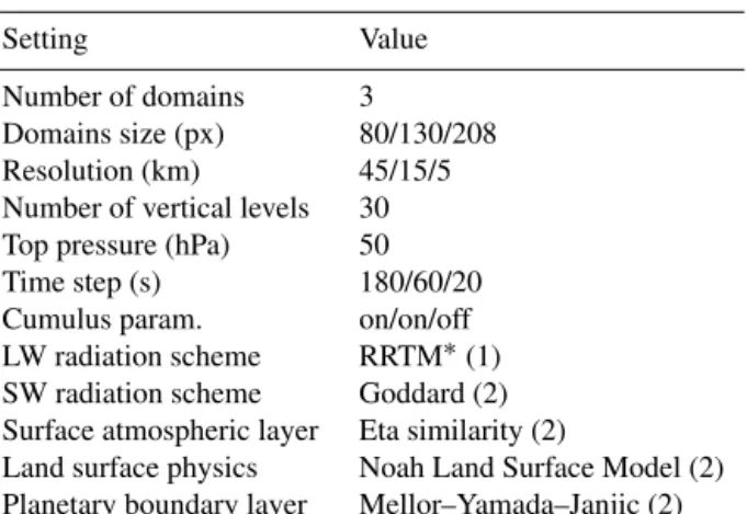
Table 1. WRF settings used for the simulations. The number in parentheses indicates the scheme number (option) in the WRF set-tings.
Setting Value Number of domains 3
Domains size (px) 80/130/208 Resolution (km) 45/15/5 Number of vertical levels 30 Top pressure (hPa) 50 Time step (s) 180/60/20 Cumulus param. on/on/off LW radiation scheme RRTM∗(1) SW radiation scheme Goddard (2) Surface atmospheric layer Eta similarity (2)
Land surface physics Noah Land Surface Model (2) Planetary boundary layer Mellor–Yamada–Janjic (2)
∗Rapid Radiative Transfer Model.
ing the boundary layer parameterization, Deb et al. (2016) showed that Polar WRF performances at the surface are most sensitive to the choice of the planetary boundary layer scheme and that the Mellor–Yamada–Janjic (MYJ) scheme is the best performer in terms of the temperature diurnal cycle (in West Antarctica) at 5 km resolution, and it is the one used in AMPS and in our study.
One of the main differences with K15 is that our simula-tion is constrained horizontally and vertically, at the bound-aries of the 45 km resolution domain, with ERA-Interim re-analysis data instead of Global Forecast System data (GFS, run by the US National Centers for Environmental Predic-tion). ERA-Interim is the latest global atmospheric
reanal-ysis (Dee et al., 2011) provided by the European Centre for Medium-Range Weather Forecasts (ECMWF). This re-analysis is based on archived observations from 1989 on-ward. It is obtained through data assimilation into an atmo-spheric model running at a resolution of 0.75 × 0.75◦, which roughly corresponds to 30 km in longitude by 80 km in lati-tude, at the latitude of Rothera Research Station (67.586◦S). Bromwich et al. (2013a) showed that using ERA-Interim re-analysis for initial and boundary conditions produces the best skills within Polar WRF.
We ran two sets of simulations. The first set spans the pe-riod 1 February 2010 to 5 March 2010, and the second set goes from 1 January 2011 to 11 February 2011 (the first two days were not included in the analysis as part of the model spin-up). These two periods cover the time of the two air-craft campaigns, including the period during 2011 when a camp was set up on the Larsen C Ice Shelf, close to auto-matic weather station 14 (AWS14; see Fig. 1b), as described in K15.
2.3 Cloud microphysics schemes
We used five different microphysics scheme to assess their ability to model realistic clouds across the Antarctic Penin-sula. None of the WRF microphysics schemes has been specifically developed for modelling Antarctic clouds. As no work has been done so far on comparing microphysics schemes implemented in Polar WRF with respect to their performances for Antarctic clouds, we used them as such with no modification. This appeared to be the most reason-able first step that can then help guide further development of Antarctic clouds microphysics modelling.
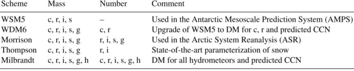
Table 2. Microphysics schemes of WRF (version 3.5.1) used in this work with their predicted cloud variables. DM stands for double-moment scheme (see text for details). All prognosed hydrometeor variables are designated by letters as follows. c: clouds droplets; i: ice crystals; r: rain drops; s: snow crystals; g: graupel; h: hail. The Morrison scheme can be used as a double-moment scheme for droplets only when WRF is used with WRF-Chem. See text for the references related to the cloud microphysics schemes.
Scheme Mass Number Comment
WSM5 c, r, i, s – Used in the Antarctic Mesoscale Prediction System (AMPS) WDM6 c, r, i, s, g c, r Upgrade of WSM5 to DM for c, r and predicted CCN Morrison c, r, i, s, g r, i, s, g Used in the Arctic System Reanalysis (ASR) Thompson c, r, i, s, g r, i State-of-the-art parameterization of snow Milbrandt c, r, i, s, g, h c, r, i, s, g, h DM for all hydrometeors and predicted CCN
Generally speaking, each scheme is a bulk microphysics parameterization (BMP) where either mass (single-moment – SM – scheme) or both mass and number density (double-moment – DM – scheme) of the various types of hydromete-ors are independently predicted. In the DM case, the scheme allows for a more realistic behaviour of clouds. Indeed, pre-dicting both the mass and the number density of hydromete-ors allows the average particle size to be predicted, which in turn allows the modelling of all size-dependent processes like sedimentation, accretion, and growth to be improved (Igel et al., 2015). All schemes have non-precipitable and precip-itable hydrometeors. The former (cloud droplets, ice crystals) are considered as having zero sedimentation velocity in the collection or accretion processes, in contrast to the latter (rain drops, snow crystals, graupel, or hail), which act as collector particles. Finally, we did not use any microphysics radius bin model (as opposed to the BMPs). They predict the evolution of cloud particles within given size bins and allow for the prediction of the actual particle size distributions. Bin mod-els are missing from WRF v3.5.1. However, a bin model is more demanding in terms of computer time, and BMPs are used in current global or regional atmospheric models and in operational forecast models like AMPS. Table 2 highlights some aspects of the cloud microphysics schemes investigated in this study.
The actual default microphysics scheme of WRF is WRF single moment 3 (WSM3), which has been discarded here be-cause it does not allow for the existence of supercooled liquid droplets. Thus, our default reference scheme is the WRF sin-gle moment 5 (WSM5), which allows for mixed-phase cloud formation (Hong et al., 2004). WSM5 is a SM scheme for all the hydrometeors. It is used in the operational model AMPS. The WRF double-moment 6 (WDM6; Lim and Hong, 2010) is an improvement on WSM5, in which droplets and rain are both treated with DM schemes, graupel is included, and all the ice phase particles are treated with a SM scheme. It is used here in order to test the improvement of the pre-diction of the supercooled liquid phase that one could expect from the use of a more sophisticated parameterization for the liquid phase (DM instead of SM as in WSM5).
The Morrison scheme (Morrison et al., 2005, 2009) is a full DM scheme for all icy hydrometeors and rain, and SM for water droplets. The Morrison scheme requires the cou-pling to the WRF-Chem module (Peckham et al., 2011) in or-der to act as a DM scheme for the cloud droplets; since such coupling was not available, we used the Morrison scheme as a SM scheme for the water droplets. This scheme is used in the Arctic System Reanalysis (ASR), which is based on Po-lar WRF as well. It slightly improved the modelling of the clouds in the northern polar summer compared to WSM5 at 30 km resolution (Wesslén et al., 2014), and this paper inves-tigates its ability to better represent the clouds in the southern polar region.
The Thompson scheme (Thompson et al., 2008) has a state-of-the art parameterization of snow, which relies on ex-tensive flight measurements, and it uses a more realistic size-dependent density for snow particles. The latter are treated as non-spherical, and their density decreases with increas-ing size. This was identified as havincreas-ing a major influence on the production of supercooled drops mainly because of a de-creased efficiency in the riming process resulting in longer-lasting supercooled drops (Thompson et al., 2008).
Finally, The Milbrandt–Yau scheme (Milbrandt and Yau, 2005a, b) (hereafter designated as Milbrandt) is a full double-moment scheme (with the shape parameters of the parti-cle distribution being fixed). It is used here in order to test the ability of a full double-moment scheme to predict su-percooled drops better than the Morrison or the Thompson schemes.
Table 3 details the way the cloud schemes treat the initi-ation of the cloud ice phase and the cloud liquid. The ini-tiation of the ice phase is the most complex part, and it re-lies on INP parameterizations. They diagnose the number of INPs, and hence the number of activated crystals, accounting for the various freezing modes described in the introduction. The INP parameterizations rely on the atmospheric temper-ature only. They are used in various ways by the different cloud microphysics schemes as illustrated in Table 3. They deal with primary ice production (droplets or vapour con-verted to ice through interaction with INPs), as opposed to secondary ice processes, which result from the interaction
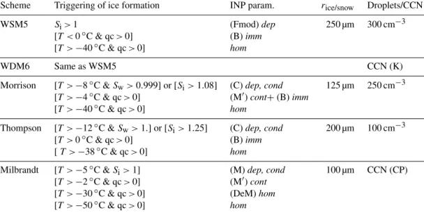
Table 3. Characteristics of the ice phase and liquid phase activation for the microphysics schemes. T refers to the atmospheric temperature, and qc to the liquid water content. Si (Sw) is the saturation ratio with respect to ice (liquid water). rice/snow indicate the cut-off size for
icy particles considered either as ice crystals (smaller particles) or snow (larger particles). INP parameterizations (INP param.) account for the various freezing processes presented in Sect. 1: imm is immersion freezing; dep is deposition freezing; cont is contact freezing: cond is condensation freezing; and hom is homogeneous freezing (considered as instantaneous, i.e. straight conversion of liquid to ice). IN/freezing parameterizations’ references: (Fmod) is a modified version of Fletcher (1962) presented in Hong et al. (2004); (C) is Cooper (1986); (M) is Meyers et al. (1992) Eq. (2.4); (M0) is Meyers et al. (1992) Eq. (2.6); (B) is Bigg (1953) for probabilistic freezing; (DeM) is Demott et al. (1994) for probabilistic freezing. CCN activation parameterizations: (K) is Khairoutdinov and Kogan (2000); (CP) is Cohard and Pinty (2000).
Scheme Triggering of ice formation INP param. rice/snow Droplets/CCN
WSM5 Si>1 (Fmod) dep 250 µm 300 cm−3
[T < 0◦C & qc > 0] (B) imm [T > −40◦C & qc > 0] hom
WDM6 Same as WSM5 CCN (K)
Morrison [T > −8◦C & Sw>0.999] or [Si>1.08] (C) dep, cond 125 µm 250 cm−3
[T > −4◦C & qc > 0] (M0) cont+ (B) imm [T > −40◦C & qc > 0] hom
Thompson [T > −12◦C & Sw>1.] or [Si>1.25] (C) dep, cond 200 µm 100 cm−3
[T > 0◦C & qc > 0] (B) imm [ T > −38◦C & qc > 0] hom
Milbrandt [T > −5◦C & Si>1] (M) dep, cond 100 µm CCN (CP)
[T > −2◦C & qc > 0] (M0) cont [T > −30◦C & qc > 0] (DeM) hom [T > −50◦C & qc > 0] hom
of already-formed crystals with other crystals or with super-cooled droplets. Finally, the liquid phase relies on a fixed number of droplets or a predicted number of activated CCN (hence number of drops), depending on the cloud scheme. At each time step, the liquid phase is formed after the ice microphysics is computed provided there is still an excess of vapour compared to equilibrium (i.e. if Sw>1, where Swis
the saturation ratio with respect to liquid water).
3 Preliminaries: results in radiation biases
Large biases in both surface downward shortwave (SW, solar flux) and longwave (LW) radiation were reported east of the peninsula over the Larsen C Ice Shelf by K15. The authors compared the summertime surface energy budget as simu-lated for January 2011 by three mesoscale models: AMPS, the UK Met Office Unified Model (UM) (see Wilson and Bal-lard, 1999, for the cloud scheme), and RACMO2 version 2.3 (see van Wessem et al., 2014, for the cloud scheme). A field camp was established close to AWS14 (see Fig. 1b) where ra-diosonde ascents allowed the water vapour column density to be calculated. AWS14 is fitted with SW and LW radiometers. K15 showed that all models mostly overestimated SW radia-tion by several tens of watts per square metre (W m−2, posi-tive bias), while they underestimated LW radiation (negaposi-tive bias). They pointed towards the lack of simulated clouds that
blocked the incoming shortwave solar radiation and emitted thermal radiation back to the surface. The only exception was noted for the UM, which had several tens of watts per square metre (W m−2) of negative bias in SW, suggesting an overes-timation of the cloud cover. AMPS simulated clouds predom-inantly composed of ice with very little or even zero liquid water, during this period over AWS14, providing an expla-nation to the very large surface radiative biases, especially in SW to which small droplets are the most responsive. Ice clouds, however, were simulated, and K15 pointed towards a misrepresentation of the actual phase of the clouds to explain the biases observed.
Following K15, Table 4 shows average biases of daily av-eraged surface downward SW and LW fluxes. They were derived by subtracting the observed value to the modelled value. Three sites were selected: the British Antarctic Sur-vey’s Rothera Research Station, on the western side of the Antarctic Peninsula, and two automatic weather stations – AWS14 and AWS15 – on the eastern side of the peninsula on the Larsen C Ice Shelf (see Fig. 1b). Both AWSs are about 70 km apart on the ice shelf. Table 4 also indicates whether the difference between WSM5 (used in AMPS) and the other schemes is statistically significant (with a Student’s t test).
Table 4. Monthly averaged shortwave (SW) and longwave (LW) surface radiative biases of daily averaged biases over Rothera, AWS14, and AWS15 for the two time periods of interest. The exponent gives the standard deviation (SD) of the daily biases. The number of “x” symbols as subscript tells how significant the difference is between WSM5 and each of the other three schemes (one, two, or three “x”s means statistical significance at the 90, 95, or 99 % level, respectively). No symbol means that the difference is not significant. Statistically significant reductions in SW/LW biases are emphasized with bold characters.
Radiation Microphysics Rothera AWS 14 AWS 15 bias scheme 2010 2011 2010 2011 2010 2011 SWSD WSM5 1568 4976 −2861 5352 −2252 4851 (W m−2) Morrison 2063 5284 −51x60 −561xxx −4352x −1250xxx Thompson 4667xx 7089 −2462 3752 −2451 2950x Milbrandt 763 4882 −3362 3156x −3050 2853x LWSD WSM5 −2825 −2626 −1128 −2023 −1029 −2220 (W m−2) Morrison −2222 −2226 225xx 121xxx 421xx 119xxx Thompson −2426 −2527 0.5x26 −621xxx 325xx −922xxx Milbrandt −1920x −1923 3xx26 −620xxx 524xx −925xx
3.1 The particular case of AWS14 in January 2011 We first compare results obtained by K15 with the AMPS model over the period 8 January 2011 to 8 February 2011 at AWS14 (see their Table 3) to our results obtained with the WSM5 scheme over the same period (Table 4, fourth column of results). Their computed biases are 56 and −10 W m−2in SW and LW, respectively. Ours are 53 and −20 W m−2, re-spectively. Discrepancies in biases can result from the com-bination of different settings in the AMPS (forcing, number of vertical levels, domain boundaries). However, we do ob-tain the same orders of magnitude and same signs of biases as K15, consistent with a lack of clouds. A striking result is that the Morrison scheme reduces the biases in both SW and LW in a statistically significant way at the 99 % level, while the Milbrandt and Thompson schemes reduce it significantly in LW only.
Figure 2 (bottom) shows the cloud liquid mass integrated over the entire atmospheric column (kg m−2) for the dif-ferent simulations as a function of time in the model grid box corresponding to the AWS14 location in 2011. Figure 2 (top) shows the simulated column density of water vapour compared to the radiosonde ascent measurements from the field camp at AWS14 (presented in K15 and plotted in their Fig. 7). The modelled water vapour is consistent with obser-vations in terms of trend and value (within ±1 kg m−2) be-tween day 8 and day 32. The simulations give similar values within ±1 kg m−2except between day 15 and day 22 (where no observation is available), and all the simulations capture the sharp increase by 6 kg m−2measured around day 28. Us-ing the Morrison scheme, 2–4 times more liquid cloud mass is simulated than when using the WSM5 scheme (Fig. 2 bot-tom). The Milbrandt and Thompson schemes lead to interme-diate amounts between WSM5 and Morrison, and WDM6 is similar to WSM5. The larger amount of liquid clouds simu-lated with the Morrison scheme compared to WSM5 is
con-sistent with its smaller SW and LW biases at AWS14 in 2011 (Table 4). This is also in line with K15’s conclusion that the thermodynamic phase of the clouds was responsible for the SW and LW biases they found in AMPS over the Larsen C Ice Shelf. The Thompson and Milbrandt schemes do have lower SW biases than WSM5 as well; however the improve-ment is smaller than with the Morrison scheme and less (or not) statistically significant. However, it is still significant for LW radiation.
The total ice mass is similar from one scheme to another, as shown by Fig. 3 (top). However an important difference arises when considering the cloud ice crystals mass only (i.e. the pristine ice – ignoring the main precipitable particles like snow and graupel particles); WSM5 and WDM6 simulate 3– 4 times more ice crystal mass than the other schemes (Fig. 3, bottom). The Milbrandt scheme leads only occasionally to as much ice mass as WSM5 and WDM6, around 19, 25, and 30 January. Graupel is mainly absent except when using the Milbrandt schemes, which leads to low amounts around 0.05 kg m−2on rare occasions (not shown). Overall, the main difference in the cloud microphysics between the various simulations at AWS14 is the ability of the cloud schemes to sustain supercooled liquid drops, which in turn can explain differences in the SW and LW surface biases. The other dif-ference lies in the distribution of the mass within the total ice phase between cloud ice crystals and snow particles. 3.2 General results in radiation biases
For the eastern side of the peninsula (AWS14 and AWS15), the biases shown in Table 4 (right part) demonstrate the importance of the choice of the microphysics scheme for the surface energy budget of the Larsen C Ice Shelf in Po-lar WRF. SimiPo-lar biases (sign and order of magnitude) are observed at a given year and for a given scheme between AWS14 and AWS15. This is consistent with the stations
be-Figure 2. (a) Time series of column density of water vapour (kg m−2) for the different simulations computed in the model grid box corre-sponding to the AWS14 location in 2011, along with the radiosonde measurements from the field camp (described in K15; see their Fig. 7). (b) Time series of the column density of the cloud liquid (kg m−2) for the different simulations.
ing 70 km apart from each other on the ice shelf, which con-sists of a relatively flat surface covered with snow and where the large-scale influences are likely to be similar in the ab-sence of significant local variations in the topography or the nature of the surface. A remarkable result is that the LW bias is significantly reduced during both periods of interest on the Larsen C Ice Shelf using the Morrison, Thompson, or Mil-brandt schemes compared to WSM5 (or WDM6 – not shown) as can be seen from the lower right part of Table 4. However, the Thompson and the Milbrandt schemes still have a nega-tive LW bias, while Morrison’s is slightly posinega-tive and gives on average the smallest LW bias at both AWS stations for both years. The standard deviation of daily averaged mea-surements remains high, but statistical tests show that the differences between WSM5 and the three other schemes are significant, mainly at the 99 % level in 2011 and mainly at the 95 % level in 2010. The SW bias is significantly reduced only with the Morrison scheme in 2011. However no improvement occurs in 2010 for the SW bias. The Milbrandt and Thomp-son schemes’ SW biases are slightly lower in 2011 with dif-ferences to WSM5 that are significant at the 90 % level. In 2010 all the schemes have a large negative SW bias, with the largest amplitude attributed to the Morrison scheme.
For the western side of the peninsula (Rothera Research Station), SW biases are always positive, and LW biases al-ways negative, whatever the cloud scheme or the year consid-ered (left part of Table 4). All simulations consistently show this imbalance, suggesting no improvement in cloud simu-lation. Furthermore, no statistically significant difference is observed between WSM5 and the other schemes. Note that almost no cloud liquid water (not shown) is simulated above Rothera (as opposed to AWS14, Fig. 2), whatever the cloud scheme used, in line with the persistent large SW and LW bi-ases. Ice and snow (graupel), however, are formed in similar amounts to the ones shown in Fig. 3 (not shown). Overall, Table 4 demonstrates the high sensitivity of the simulated downward radiation fluxes to the microphysics scheme used in Polar WRF.
A major issue in assessing the performances of the cloud microphysics schemes by investigating radiation biases is that it does suppose that the appropriate information is passed on from the cloud scheme to the radiative scheme. This as-pect can explain the apparent paradox of the significant im-provement of the LW bias to the east of the peninsula with three schemes, while no concomitant SW bias improvement is being observed. The discrepancies in SW and LW bias improvements will be further discussed in Sect. 5.1. Radia-tive schemes themselves also require careful examination as they also rely on various assumptions and simplified geom-etry to retrieve SW and LW fluxes. The radiative schemes that we used were chosen for consistency with K15 in order to compare their conclusions (using AMPS) to ours (using Polar WRF). We do not intend here to investigate the radia-tive schemes implemented in WRF. For further assessment of cloud microphysics schemes’ performances and behaviours
at a much wider scale, we now compare the simulation out-puts to each other and to the cloud microphysics properties as measured during the BAS aircraft campaigns that took place over the Antarctic Peninsula (presented in part 1).
4 Results: simulated clouds as compared to observations
4.1 General trends for simulated clouds across the peninsula
The topography of the Antarctic Peninsula (Fig. 1) makes it interesting to focus on zonal distribution of latitudinal av-erages for the LWC (in g kg−1) and the solid-water content (SWC, g kg−1). SWC comprises ice, snow, and graupel mass. It is different from the IWC, which consists only of the mass of the cloud ice crystals. LWC and SWC were respectively averaged between latitudes 65.5 and 68.5◦S and altitudes below 4500 m. This geographical area includes the region where both flight campaigns took place in summer 2010 and 2011 (Fig. 1b). For simplicity we designate each simulation by using the name of its cloud microphysics scheme.
Both periods of interest display the same relative trends, and we present an average over both periods to give an overview. Averages are computed considering either all val-ues, including null instances (LWC0and SWC0 in Fig. 4a
and b, respectively), or only strictly positive values (LWC and SWC in Fig. 4c and d, respectively). Thus, we always have LWC0≤LWC and SWC0≤SWC. LWC (SWC) gives
the liquid (ice) content that is simulated disregarding how often the clouds form. LWC0(SWC0) describes a more
real-istic average behaviour since it also accounts for the ability of the scheme to lead to liquid (ice) cloud formation, more or less often.
For all the simulations, LWC and LWC0 are in the
inter-val 0.05–0.14 and 0.002–0.03 g kg−1, respectively. SWC and SWC0are in the interval 0.02–0.08 and 0.01–0.035 g kg−1,
respectively. The lower limit of LWC0(0.002 g kg−1) is due
to WSM5’s cloud liquid mass decreasing over the moun-tains down to 0.002 g kg−1around 65◦W. For the other cloud schemes, LWC0≥0.01 g kg−1. There is roughly a factor of
5 to 10 between LWC0and LWC, while there is a factor of
1.2 to 2 between SWC0and SWC. The liquid phase features
more important changes (from null to non-null values) than the total ice phase, which is simulated more frequently.
WSM5 strikingly differs from the Morrison, Thompson, and Milbrandt schemes in that its LWC and LWC0
de-crease above the peninsula’s mountains. LWC drops from ∼0.12 g kg−1by more than 50 % from 70 to 65◦W, before increasing back from 65 to 60◦W to ∼ 0.12 g kg−1(Fig. 4c). Except east of 62◦W, where WDM6’s LWC is larger than WSM5 by less than 0.03 g kg−1(not shown), both schemes display very similar averages for LWC and SWC, and we only show WSM5. LWC is much steadier for the three other
Figure 4. Longitudinal distribution of latitudinally (65.5–68.5◦S) averaged LWC and SWC (g kg−1) over both periods of interest for the WSM5, Morrison, Thompson, and Milbrandt schemes. The average is computed over all grid boxes and times, leading to (a) LWC0and
(b) SWC0, or only over grid boxes and times where values are non-null, leading to LWC (c) and SWC (d). The thick grey line shows the
surface height averaged over the same region and labelled on the right vertical axis of each plot. Note the identical scales used for the vertical axes for LWC0and SWC0and for LWC and SWC.
schemes, and a sharp increase for the Milbrandt and Morri-son schemes is observed above the highest terrains, caused by the orographic forcing induced by the westerlies or the easterlies (see Sect. 4.2).
The first obvious assessment with respect to the ability of the cloud schemes in forming (supercooled) liquid clouds is that WSM5 (WDM6) leads to less supercooled liquid mass than the Morrison, Thompson, and Milbrandt schemes across the Antarctic Peninsula. Eastward of 62◦W, WSM5’s LWC0 is 100 % (50 %) smaller than Morrison’s
(Thomp-son’s), while it is similar to Milbrandt’s (Fig. 4a). How-ever, in the central region over the mountains, WSM5 (and WDM6) leads to less liquid mass by up to an order of magni-tude than the three other schemes. Westward of 69◦W LWC0
is similar for WSM5, Milbrandt, and Thompson; they are all twice as small as Morrison’s LWC0. WSM5 does not lead
as often as the other schemes to supercooled liquid forma-tion, which is illustrated by its lowest LWC0 values, yet it
does simulate as large average liquid water contents as the other schemes when and where liquid forms (similar LWC), except in the central region, where orographically induced
clouds have systematically less liquid water. The ice phase instead shows a similar behaviour across the different cloud schemes with an increasing SWC closer to the high-altitude topography, due to orographic forcing. SWC0 is similar for
WSM5, Morrison, and Thompson, while with Milbrandt it reaches 50 % larger value largely due to the graupel mass (not shown).
Comparing LWC0 and SWC0, we see that the
simula-tion with the Morrison scheme is the only one sustain-ing supercooled liquid mass more frequently than ice mass (LWC0>SWC0 by a factor of > 1 to 2). For the
Thomp-son scheme, LWC0∼SWC0on average (but LWC0<SWC0
over the mountains, and LWC0>SWC0east of the Larsen C
Ice Shelf). The Milbrandt scheme leads more often to ice mass formation than liquid mass (LWC0<SWC0) by a
fac-tor of less than 2 at all longitudes, and WSM5 by a facfac-tor of 1 to 5. Finally, the simulation with WSM5 (WDM6) is the only one resulting in an anticorrelation between LWC (LWC0) and SWC (SWC0) with an increase (decrease) for
Figure 5. Transect of the cloud microphysics for WSM5 (a, b) and Morrison (c, d) averaged over a period (7–10 January 2011) dominated by westerly winds (a, c) and over another period (11–17 January 2011) dominated by easterly winds (b, d). The transect is approximately centred on Rothera Research Station (67.586◦S), and it is an average over a 100 km wide latitudinal band. The longitudes of Rothera, AWS14, and AWS15 are indicated.
4.2 Dynamics and microphysics structure of the simulated clouds
The Antarctic Peninsula’s mountains act as a barrier to the westerly or easterly winds that drive the formation of oro-graphic clouds. As a complement to the general picture given above, we identified one period of sustained westerly wind regime and one period of sustained easterly wind regime. We isolated the period 7 to 10 Januray 2011, when west-erlies prevailed almost exclusively, and similarly the period 11 to 17 Januray 2011, when the easterly regime prevailed. Note that the average wind directions and speed, and their relative variations, are in agreement with upper-air measure-ments performed daily from Rothera Research Station (not shown), if not always quantitatively at least qualitatively, as well as with measurements from the aircraft (not shown).
Figure 5 shows time- and space-averaged transects of the hydrometeors’ mass (including null instances) across
the peninsula on a ∼ 100 km wide (67–68◦S) latitudinal band approximately centred on Rothera Research Station, for WSM5 (Fig. 5a and b) and the Morrison scheme (Fig. 5c and d). The westerly cases (panles b and d) and easterly cases (panels a and c) show the orographic clouds microphysical structure. They also illustrate the very different contexts of Rothera Research Station on the western side and of AWS14 and AWS 15 on the eastern side. Rothera itself is in the lee of a mountainous feature (Adelaide Island), and the topography adds to the complexity in simulating the clouds compared to the flat Larsen C Ice Shelf.
WSM5 predicts completely glaciated clouds on the penin-sula and liquid clouds only away from the mountains with a very limited vertical extent (up to 500 m above the sur-face). The Morrison scheme maintains mixed-phase clouds across the region and at much higher altitudes. This fact alone is in better agreement with observations from the aircraft, which measured almost exclusively mixed-phase
clouds (part 1). Over the ice shelf the snow increases from 0.01 to 0.05 g kg−1as we get closer to the mountain barrier for all the schemes (similar amounts are simulated on the western side during the westerly regime). However, WSM5 simulates an IWC (orange lines) as large as the snow parti-cles mass (red lines) down to the surface, contrasting very much with the Morrison scheme.
Note that WDM6 (not shown) gives similar results to WSM5. Also, the microphysical structure of the clouds pre-dicted by the Thompson scheme and the Milbrandt scheme (not shown) are similar to the Morrison scheme. On ei-ther side of the peninsula, downwind, the Morrison scheme forms the most abundant mixed-phase cloud layer with LWC ∼ 0.1 g kg−1, and the clouds extends almost down to the surface (LWC ∼ 0.01 g kg−1), whereas the Milbrandt and Thompson schemes form less than half of that maximum amount, in line with the general picture given in Sect. 4.1. Also, the Milbrandt scheme forms a significant amount of cloud ice crystals (IWC) above 3000 m, as well as graupel in the mixed-phase orographic clouds above the windward slopes (not shown), which are absent from the average tran-sects of the Morrison and Thompson simulations.
4.3 Microphysics schemes performances west and east of the Antarctic Peninsula
4.3.1 Liquid phase
To assess the performances of the different cloud schemes, we compare the LWC measured from the aircraft to the sim-ulated LWC by restraining the latter to the model grid boxes corresponding to the flight tracks. We only consider non-null LWC values (LWC > 0.001 g kg−1). For each data point, the closest (both in time and space) grid box value is extracted from the model. Latitudinal averages are derived for each flight per 0.5◦ longitude bins, for simulations and observa-tions. At the latitude of Rothera Research Station (67.586◦S) this corresponds to ∼ 10 km (i.e. two grid boxes). Then, global west and east averages are derived, corresponding to longitudes westward of 67◦W and to longitudes eastward of 65◦W, respectively (as in part 1). LWC is derived as pre-sented in part 1 using the droplet size distribution obtained from the CAS.
The unknown thermodynamic phase of the smallest parti-cles seen – but not resolved – by the CIP, and that can be ei-ther drops or small crystals (see part 1), may induce a bias in the derivation of LWC. However, if all of them were counted as droplets, they would increase LWC by ≤ 8 % for all flights except two flights in 2010 (13 and 30 %) and one flight in 2011 (12 %). This bias does not alter the results or the con-clusions below. More information on the instruments and the measurement can be found in part 1 (their Sect. 2.1).
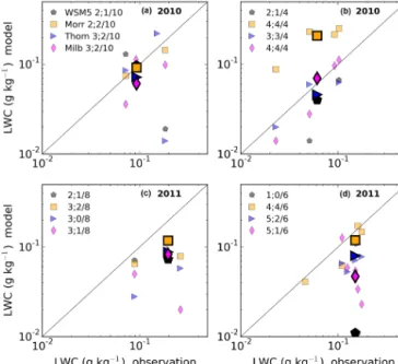
Figure 6 shows the scatter plots of simulated LWC versus observed LWC for 2010 (Fig. 6a and b) and 2011 (Fig. 6c and d) and for either side of the peninsula, west (panels a and c)
Figure 6. Scatter plot of simulated LWC versus observed LWC in 2010 (a, b) and in 2011 (c, d) on the western side of the penin-sula (a, c) and on the eastern side of the peninpenin-sula (b, d). Light markers show averages per flight track, while bold markers give the average of all the tracks on each side of the peninsula. The numbers next to each scheme’s marker in the legend (n5; n50/N) gives the
number n5(n50) of simulated flights with a simulated LWC at least 5 % (50 %) of the observed LWC to the total number N of flights measuring an average LWC. Note that in panel (c) the bold markers (total average) overlay some light markers (flight averages), which explains the actual higher position of the total average on the graph compared to the other discernible lower flight averages.
and east (panels b and d). Regional (east or west) averages are represented by the largest bold markers, while smaller mark-ers relate to individual flight averages. Note that the width of the large markers is larger than the length of the error bar associated with the aforementioned error (bias) related to the LWC derivation. The numbers shown next to each scheme’s markers in the legend (in the form n5; n50/N) indicate the
number of flight tracks for which the simulation forms at least an average of 5 % (n5) or 50 % (n50) of the observed
av-erage LWC, over the total number of flight tracks (N ) having measured cloud liquid. We refer to those as the n5criterion
and the n50criterion, respectively.
Three results stand out. First, all the schemes perform worse in the west than in the east in terms of number of tracks with simulated clouds (n5and n50criteria) except for
the WSM5 scheme, which performs equally bad on both sides. Second, the WSM5 scheme has the lowest numbers of flights with some liquid clouds simulated (n5 criterion).
For the Morrison, Thompson, and Milbrandt schemes, about (Fig. 6a) or much less than (Fig. 6c) 30 % of flights are pre-dicted with some substantial supercooled liquid (n50
(Fig. 6b and d). Third, the Morrison scheme performs on av-erage the best in reproducing observed LWC in the western and the eastern portions of the flight tracks, with larger values of LWC simulated than for the other schemes. When consid-ering the n5criterion, the Thompson and Milbrandt schemes
show equally good scores compared to Morrison, suggesting the same ability to initiate a non-negligible supercooled liq-uid phase, as opposed to WSM5 (and especially on the east-ern side). However, overall the Morrison scheme performs better because it has an averaged simulated LWC closer to the observed one within a factor of less than 2 (except in the east in 2010 – Fig. 6b – where it simulates an average LWC 3 times larger than the observations).
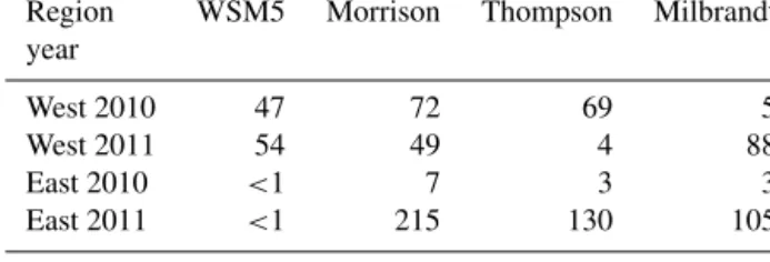
Those averages do not take into account the duration over which such values are observed. Thus, we use an additional metric that is the average time spent in cloud (or instances of cloud occurrences) on either side of the peninsula. The av-erage ratio of the time spent in clouds in the model (with LWC > 0.01 g kg−1) over the one in the measurements is given in Table 5 for each side and year. The average is de-rived as an average of the flight averages. Over both periods the best scheme appears to be the Morrison scheme since the Thompson and Milbrandt schemes have very low occur-rences of clouds compared to the observation on the western side, with 4% in 2011 and 5% in 2010, respectively. On the eastern side, WSM5 has the poorest performance (< 1 %), and the Morrison scheme has twice as many occurrences of clouds (although still quite low) in 2011 as the two other schemes, and it overpredicts the formation of clouds in 2011 (215 %), although not the average LWC (Fig. 6d).
Average vertical profiles of cloud liquid (and ice) were also derived for flights measurements as well as for the model outputs. The altitude grid on which flights observa-tions, and model outputs, were averaged is finer in its lower layers, with one level every 100 m below 1100 m and ev-ery 200 m above 1100 m. At each altitude level the aver-age of the flight averaver-ages is computed so that every flight has the same weight. Model altitude levels are separated by less than 1000 m at the highest altitude levels of the atmo-spheric column. However, below 4500 m, where the flights took place, the maximum model level separation is approx-imately 500 m. Thus, any data point level is less than 250 m away from the closest model level (less than 100 m below 1100 m). Figure 7 compares vertical distribution of observed (grey circles) and simulated (coloured markers) non-null av-erage LWC (> 0.001 g kg−1) for WSM5 (top) and the Morri-son scheme (bottom). The grey shaded area shows the spread of all flight averages. The error bars show the spread of the simulated flight averages. The numbers at each level indicate how many simulated flights with non-null averages are used to derive the total average of each level, for the simulations as compared to (“/”) the observations.
The WSM5 scheme does not form liquid clouds above 800 m on the western side of the peninsula or above 500 m on the eastern side during both periods of interest. Liquid clouds
Table 5. Average ratio (%) of the number of occurrences of LWC > 0.01 g kg−1in the simulations over the observations. The average is derived from the flight averages.
Region WSM5 Morrison Thompson Milbrandt year
West 2010 47 72 69 5
West 2011 54 49 4 88
East 2010 <1 7 3 3 East 2011 <1 215 130 105
were observed as high as 4400 m. The numbers at each level show that WSM5 simulates fewer occurrences of liquid than the Morrison scheme, which still underpredicts the occur-rences of liquid clouds. The Morrison scheme shows liquid cloud formation up to 2500 m, albeit only very few instances above 1500 m.
WDM6 shows no improvement compared to WSM5 (not shown). The Milbrandt and Thompson schemes simulate liq-uid clouds more often than WSM5 in the lowest layers, but no clear systematic difference emerges between those two and the Morrison scheme. The Morrison scheme simulates best the increasing trend of LWC with altitude in the west in 2011. It has the largest LWC below 1000 m (by 0.1–0.2 g kg−1) on either side of the peninsula in 2010 compared to other schemes, while LWC is comparable for all the three schemes in 2011 (not shown).
4.3.2 Ice phase and mixed phase
For completeness we compare the simulated SWC (g kg−1) to the observed ice mass. Figure 9 is the same as Fig. 6 but for SWC, with the addition of the corresponding IWC re-gional averages shown as large light grey markers. (The latter are slightly shifted rightwards by 50 % of the observed value on the x axis in order to be visible.) The smaller and light-coloured markers are individual flight averages. The same n5
criterion and n50criterion as in Fig. 6 are used and referenced
in Fig. 9 next to each cloud scheme’s name.
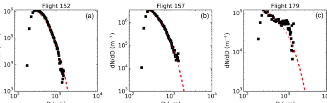
As mentioned in part 1, there is an uncertainty in the small-est particles detected by the CIP; however they contribute to a negligible amount of the total measured ice mass. At the other end of the size distribution, the maximum cut-off for detected ice particles is about 1.5 mm in size (di-ameter). Thus possible larger particles that could signifi-cantly add to the mass are not detected. However, in or-der to have an estimate of the error caused by the missed larger particles, we approximated and extrapolated the av-erage size distribution of the crystals for each flight (ex-amples are shown in Fig. 8a and b), using an exponential distribution of the form N (D) = N0exp(−λD) (known as
Marshall–Palmer distributions) commonly used for the rain and the ice hydrometeors in the cloud microphysics schemes (e.g. Morrison et al., 2009). Using the exponential
distribu-Figure 7. Averaged vertical profiles of non-null LWC for WSM5 (a–d) and the Morrison scheme (e–h) and for the observations west (a, b, e, f) and east (c, d, g, h) of the peninsula. Grey markers indicate the measured average at each altitude, while the shaded area gives the range of the observed flight averages at each altitude. Similarly, coloured markers and error bars relate to the cloud schemes. The numbers indicate how many simulated flight averages were used to derive the global average at each altitude for each scheme, as compared to (“/”) for the observations.
Figure 8. Average size distribution of the crystals identified with the CIP for the flights (a) 152, (b) 157, and (c) 179 (black squares), along with the exponential distribution approximating them (red dashed line). The relative increase in ice mass when further integrating from 1.5 mm to larger diameters (equal to the relative error on the actual ice mass used in this study) is about 3 % (a), 2.5 % (b), and 65 % (c) (see text for details).
tion and the mass-diameter law, we derive an ice water con-tent below 1.5 mm and above 1.5 mm, respectively. In order to derive the mass for D ≤ 1.5 mm, we integrated over the crystal sizes starting from the peak diameter of the distribu-tion and up to 1.5 mm. The peak diameter of the observed ice crystal distribution is located in the range 250–425 µm (with an average of 315 µm), a value from which the expo-nential distribution can approximate the distribution of the largest crystals. Then, the ice water content for particles with D >1.5 mm, and up to an arbitrary limit of 3.2 mm, was de-rived (setting the upper limit to even larger sizes does not change the resulting additional ice mass given the even lower amounts of crystal number concentration predicted by the ex-ponential distribution). The ratio of both ice water contents allows estimating the relative error caused by the undetected
particles on the measured SWC when assuming an exponen-tial distribution. For the 2010 flights, this average error is about 5 %, including an outlier flight with a 33 % error (ig-noring this flight brings the average error to 2 %). For the 2011 flights, the average relative error is about 8 %, includ-ing an outlier with a 65 % error (shown in Fig. 8c) (ignorinclud-ing this flight brings the average error to 2 %). The large error de-rived for the two flights is related to a shoulder of the crystal distribution for the larger particles, leading to an exponential distribution predicting a number concentration of the largest particles likely to be in large excess compared to the actual one (Fig. 8c). Overall, these estimates of the relative errors in SWC do not alter the main conclusions presented here.
Table 3 gives the cut-off radii between ice particles and snow particles in the different cloud schemes. The different
Figure 9. Scatter plot of simulated solid-water content (SWC; ice, snow, graupel) versus observed SWC in 2010 (a, b) and in 2011 (c, d) on the western side of the peninsula (a, c) and on the eastern side of the peninsula (b, d). The small light-coloured mark-ers show the average per flight, while large coloured bold markmark-ers give the average over the whole tracks on each side of the peninsula. The large light grey markers show the simulated ice water content (IWC) averages corresponding to each simulated SWC average (for readability each light-grey marker is slightly shifted on the x axis by 50 % of the measured value). The numbers next to each scheme’s name (n5; n50/N ) give the number n5(n50) of simulated flights
with a SWC of at least 5 % (50 %) of the observed SWC to the total number N of flights measuring an average ice content of at least 0.0001 g kg−1.
definitions of the icy hydrometeors across the cloud schemes add to the difficulty of performing comparisons between the schemes as well as the observations. The observed particles identified unambiguously as crystals in part 1 span the di-ameter range 200 µm to 1.5 mm. Hence, because the cloud microphysics schemes have a lower limit size smaller than 200 µm for the ice crystal and an upper limit size larger than 1.5 mm for the precipitating ice particles (snow, graupel ;see Table 3), we expect the simulated IWC and SWC to bracket the observations. However, the measured ice mass should be closer to SWC than to IWC given the relatively low addi-tional mass expected from particles with D > 1.5 mm using the estimates presented above.
In 2010, the instances where SWC and IWC do bracket the observations happen on both sides of the peninsula (Fig. 9a and b) for the Morrison and Thompson schemes (note that the Thompson scheme’s IWC is between 10−4and 10−3g kg−1). WSM5’s SWC and IWC equal the observation, showing that a significant part of the simulated SWC is on average in the form of cloud ice crystals (IWC) (i.e. radii < 250 µm; see
Ta-ble 3). In 2010, west of the peninsula, Milbrandt’s SWC and IWC are lower than the observations, suggesting not enough ice formation.
In 2011 (Fig. 9c and d), all the scheme have both aver-aged SWC and IWC lower than the observations, except for WSM5 to the east of the peninsula, where the averaged IWC exceeds the observed value. East of the peninsula, all the schemes predict equally well some non-negligible ice phase (n5criterion), with Morrison, Thompson, and Milbrandt
per-forming better than WSM5 when considering the n50
crite-rion. However, the schemes perform worse west of the penin-sula, with less than 40 % of ice occurrences actually sim-ulated (n5 criterion). Overall, As for the liquid phase, the
occurrences of the ice phase are less well simulated on the western side of the peninsula than on its eastern side.
Finally, we focus on the partition of water between the condensed phases, LWC, and SWC by looking at the total average mixed-phase ratio fm=LWC/(LWC + SWC) as a
function of temperature along the flight tracks. Table 6 sum-marizes the statistics on fmderived from measurements and
from simulations. First, none of the schemes sustain liquid clouds at temperatures below −15◦C, or even below −9◦C for the WSM5 (WDM6) scheme (leading to fm=0). This
will be further commented on in Sect. 5.2. Second, between −15 and 0◦C, the Morrison scheme (0.91 ± 0.1) and the Mil-brandt scheme (0.78 ± 0.1) have an average fm in closest
agreement with observations (0.83 ± 0.08). WSM5 performs the least well, with fm around 0.6 on average and down to
0.07 at its minimum. WSM5 (σ = 0.24) and the Thomp-son scheme (σ = 0.2) have a variability of fm more than
twice as large as the observations (σ = 0.08). Practically, for WSM5 and the Thompson scheme, it results in a highly vari-able mixed-phase ratio from one 0.5◦temperature bin to the
next, which is not observed in the measurements (not shown). The Morrison scheme (σ = 0.1) and the Milbrandt scheme (σ = 0.1) have a steadier fmacross the investigated
tempera-ture range where mixed-phase clouds are simulated, in closer agreement to the observations.
4.4 Temperatures and water vapour in Polar WRF over the flight campaigns
We take advantage of temperature and water vapour mea-surements performed along with the cloud in situ measure-ments to compare with the averaged simulation outputs. Lat-itudinal averages (in 0.5◦longitude bins) for both observa-tions and simulaobserva-tions are shown for temperatures (◦C) and
water vapour mass mixing ratios (g kg−1) in Fig. 10a and b, respectively. The variability of the water vapour and of the temperature (shown as the standard deviation of the flight averages in each longitude bin) is indicated with shaded area for the observations and with error bars for the different cloud schemes. The measurement uncertainty for the temperature measured with a Rosemount probe is about 0.3◦C (Stickney et al., 1994), corresponding to less than the width of the solid
Table 6. Statistics over the flight tracks on the mixed-phase ratio fm=LWC / (LWC + SWC) for temperatures T > −15◦ (see text
for details).
fm Observation WSM5 Morrison Thompson Milbrandt
Average 0.84 0.6 0.91 0.66 0.79
σ 0.08 0.24 0.1 0.20 0.10
Max 0.94 0.9 1 0.92 0.95
Min 0.60 0.07 0.61 0.21 0.56
blue and red lines. The darkest narrow shaded areas brack-eting solid lines on both years correspond to a conservative estimate of uncertainty on water vapour (±0.15 g kg−1) as derived using the relative humidity measured with a Vaisala HUMICAP HMP45 (±3 % estimated relative error) and the atmospheric temperature measurements from the Rosemount probe. A Buck 1011C cooled-mirror hygrometer also present on board was used to correct for an offset in the HUMI-CAP measurements. At low temperatures and humidity the cooled-mirror hygrometer occasionally has difficulty in iden-tifying the frost point correctly and tends to hunt over a wide range. Therefore the HUMICAP measurements were used once corrected using the cooled-mirror hygrometer during periods when we are confident that it has correctly identified the frost point.
For the temperature, in 2010 all the simulations show best agreement with the measurements to the east of the penin-sula, where the overestimation of the temperature ranges be-tween 0 and 1◦C (Fig. 10a, top). Westward of 65◦W the pos-itive biases are larger and range between 1 and 2◦C. In 2011 and east of the peninsula, the temperature bias lies between 1 and 2◦C, whereas west of 69◦W it ranges between 2 and
3◦C with the exception of the Thompson scheme leading to overestimations as large as 4◦C (Fig. 10a, bottom).
For the water vapour, the 2011 observed average is un-derestimated at almost all longitudes except between 68.5 and 64◦W, where it is overestimated by 0.15 g kg−1on av-erage (Fig. 10b, top). Eastward of 63◦W, the underestima-tion increases up to values closer to 1 g kg−1, while west-ward of 71◦W it remains around 0.5 g kg−1. In 2010 the average water vapour is underestimated by 0.2–0.5 g kg−1, except west of 68◦W where it reaches 1 g kg−1 (Fig. 10b, bottom). The bias then decreases to around 0.25 g kg−1 in the area 67.5–63.5◦W, except for WSM5, which remains closer to 0.5 g kg−1. Eastward of 62◦W the underestimation increases up to 1 g kg−1, but only one flight measured water vapour, hence the poor statistics (as shown by the absence of shaded area). WSM5 has the largest biases in averaged water vapour during both years, 0.6 and 0.45 g kg−1in 2010 and 2011, respectively, mostly consisting of an underestima-tion of the observed water vapour. Other schemes also mostly underestimate the water vapour, albeit less than WSM5 by 0.05–0.1 g kg−1. No cloud scheme clearly stands out in terms of reducing the negative bias.
Figure 10. Zonal distribution for 2010 and 2011 flight campaigns of averaged (a) temperature and (b) water vapour (g kg−1). Mea-surements are shown as a solid line, and simulations as markers. Shaded areas and error bars give the standard deviation in each 0.5◦ longitude bin for the observation and the simulations, respectively. The dark shaded area corresponds to a conservative estimate of the uncertainty on water vapour (see text for details).
Overall across the peninsula the simulations underesti-mate the measured water vapour by an average value of 0.5 g kg−1 (±0.2 g kg−1, depending on schemes or regions across the peninsula), and the temperatures are overestimated by 1◦C (±0.2◦C, depending on the scheme) in 2010 and 2◦C (±0.5◦C, depending on the scheme) in 2011. Interest-ingly, the variabilities of the observations (shaded area) and of the simulations (error bars) are consistent with each other. This suggests a good performance of the model average and variability. The broad agreement in temperature and water vapour between the simulations suggests that their differ-ences in average simulated clouds cannot be mainly related to the differences in water vapour and temperature, but rather to their microphysics. The biases compared to the observation will be further commented on in the Sect. 5.4.