Upscaling of land-surface parameters through direct moment propagation

HAL Id: hal-00296853

https://hal.archives-ouvertes.fr/hal-00296853

Submitted on 16 Dec 2005

HAL is a multi-disciplinary open access

archive for the deposit and dissemination of

sci-entific research documents, whether they are

pub-lished or not. The documents may come from

teaching and research institutions in France or

abroad, or from public or private research centers.

L’archive ouverte pluridisciplinaire HAL, est

destinée au dépôt et à la diffusion de documents

scientifiques de niveau recherche, publiés ou non,

émanant des établissements d’enseignement et de

recherche français ou étrangers, des laboratoires

publics ou privés.

Upscaling of land-surface parameters through direct

moment propagation

H. Kunstmann

To cite this version:

H. Kunstmann. Upscaling of land-surface parameters through direct moment propagation. Advances

in Geosciences, European Geosciences Union, 2005, 5, pp.127-131. �hal-00296853�

Advances in Geosciences, 5, 127–131, 2005 SRef-ID: 1680-7359/adgeo/2005-5-127 European Geosciences Union

© 2005 Author(s). This work is licensed under a Creative Commons License.

Advances in

Geosciences

Upscaling of land-surface parameters through direct moment

propagation

H. Kunstmann

Institute for Meteorology and Climate Research (IMK-IFU), Forschungszentrum Karlsruhe, Kreuzeckbahnstraße 19, 82467 Garmisch-Partenkirchen, Germany

Received: 7 January 2005 – Revised: 1 August 2005 – Accepted: 1 September 2005 – Published: 16 December 2005

Abstract. A new methodology is presented that allows the upscaling of land surface parameters of a Soil-Vegetation-Atmosphere-Transfer (SVAT) Model. Focus is set on the proper representation of latent and sensible heat fluxes on grid scale at underlying subgrid-scale heterogeneity. The ob-jective is to derive effective land surface parameters in the sense that they are able to yield the same heat fluxes on the grid scale as the averaged heat fluxes on the subgrid-scale. A combination of inverse modelling and Second-Order-First-Moment (SOFM) propagation is applied for the derivation of effective parameters. The derived upscaling laws relate mean and variance (first and second moment) of subgrid-scale heterogeneity to a corresponding effective parameter at grid-scale. Explicit upscaling relations are exemplary de-rived for a) roughness length, b) wilting point soil moisture, and c) minimal stomata resistance. It is demonstrated that the SOFM-Method yields congruent results to corresponding Monte Carlo simulations. Effective parameters were found to be independent of driving meteorology and initial conditions.

1 Introduction

Mesoscale distributed hydrological models as well as process-based regional climate models often use grid reso-lutions that are not able to account for detailed land surface heterogeneity (e.g. soil, vegetation and land surface proper-ties). The impact of this subgrid-scale heterogeneity usually is not accounted for. Land surface information, however, of-ten is available in higher spatial resolution than the specific model resolution (e.g. via satellite data) and the coarse model resolution is only due to limited CPU resources. If subgrid-scale effects shall be accounted for on grid-subgrid-scale, aggregation techniques have to be applied that allow the derivation of ef-fective model parameters.

Correspondence to: H. Kunstmann

(harald.kunstmann@imk.fzk.de)

The upscaling of land surface parameters in this study re-lates to the physical description of energy and water bal-ance at the land surface according to the equations of the Soil-Vegetation-Atmosphere-Transfer (SVAT) model of the Oregon State University (OSU-LSM) (Ek and Mahrt, 1991; Chen and Dudhia, 2001). The OSU-LSM provides the lower boundary condition of the non-hydrostatic mesoscale mete-orological model MM5 (Grell et al., 1994). MM5 usually is applied in horizontal resolutions of 10×10–50×50 km2. This resolution in most cases is too coarse to account for vari-ability in surface parameters like albedo, emissivity, rough-ness length or vegetation parameters like stomatal resis-tances. SVAT-models, both in stand-alone versions and those coupled to regional climate models, provide tabulated values for land surface parameters dependent on soil and vegetation type, however, independent of scale (i.e. horizontal model resolution). The question arises, how these land surface pa-rameters must be chosen dependent on the scale (i.e. the hor-izontal model resolution) such that modelled heat fluxes at grid scale equal aggregated heat fluxes at subgrid scale.

Explicit scaling laws for central land surface parameters are derived that relate mean (1st moment) and standard devi-ation (2nd moment) of subgrid scale parameter distribution to a corresponding effective parameter value at grid scale. Ef-fective parameters are derived by a combination of first mo-ment propagation and inverse modelling. It is in particular shown that the Monte Carlo based approach (as introduced by Intsiful, 2004) and the direct first moment propagation approach (based on a Taylor-Series expansion) of this work yields identical results.

2 The SVAT model – brief overview

The SVAT model applied in this study closely follows the ap-proach of Ek and Mahrt (1991) and Chen and Dudhia (2001). It solves the energy balance

128 H. Kunstmann: Upscaling of land-surface parameters through direct moment propagation with Rn: net radiation [Wm−2], G: ground heat flux

[Wm−2_{], λE: latent heat flux [Wm}−2_{], H : sensible heat flux}

[Wm−2_].

Net radiation is obtained by

Rn=(1 − α)SWin+LWin−ε · σ · tsfc4 (2)

with α: albedo [.], ε: emissivity [.], SWin:

incom-ing shortwave radiation [Wm−2_{], LW}

in: incoming

long-wave radiation [Wm−2], σ : Stefan-Boltzmann constant [5.67 10−8Wm−2K−4], tsfc: temperature of land surface

[K].

The model has the prognostic variables soil temperature, volumetric soil water content, canopy water content and the diagnostic variables sensible heat flux, latent heat flux (from canopy, stomata and bare soil), ground heat flux, infiltration excess. The soil is discretized in four layers with vertical res-olutions 10 cm, 30 cm, 60 cm, and 100 cm. Soil thermody-namics is accounted for by solving the heat flux equation, in which volumetric heat capacity depends on actual volumet-ric soil content. Soil moisture dynamics in the unsaturated zone is described by solving the diffusive form of Richard’s equation. Soil hydraulic conductivity, hydraulic conductiv-ity and matric potential nonlinearly depend on the Clapp-Hornberger parameter b (a curve fitting parameter dependent on soil type). Canopy transpiration is calculated dependent on vegetation fraction, canopy resistance, canopy water con-tent and pocon-tential evaporation. Canopy resistance nonlin-early depends on leaf area index (LAI), minimum (Rcmin)

and maximum stomatal resistance, solar insolation, vapour pressure, atmospheric temperature and soil moisture content. When the soil moisture exceeds the field capacity θref,

tran-spiration is not regulated by soil moisture deficit. When the soil moisture is less than wilting point soil moisture θwilt,

soil water deficit prevents transpiration. Aerodynamic rough-ness length (z0 m)determines the zero-wind level in the

verti-cal logarithmic wind profile of the planetary boundary layer (PBL); as it non-linearly impacts canopy resistance it is very sensitive to latent heat flux.

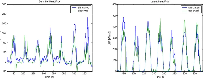
The SVAT-model is programmed in Mathematica (Wol-fram, 2004) and applied and validated using forcing and observation data from Meyers/NOAA measurement site in Champaign, Illinois. The measurement site is located at 88.37◦_{W and 40.01}◦_{N. Data are available for the scientific}

community and can be retrieved via ftp://ftp.ncep.noaa.gov. The site is characterised by soil type “silty loam” and veg-etation type “groundcover only”. This study focuses on Ju-lian days 195–200 in 1998. A comparison between mod-elled and observed sensible and latent heat fluxes are given in Figs. 1a, and b. The SVAT model in general reproduces well observed daily variation of heat fluxes. Time resolution 1twas 15 min.

3 Upscaling methodology

Figure 2 illustrates the general methodology applied for de-riving effective parameters. In a square of n gridpoints at

subgrid scale, every grid point i is characterised by a dif-ferent land surface parameter pi (i=1,. . . , n). In our case,

p can for example represent albedo, emissivity, roughness length or any other land surface parameter of interest. The SVAT model calculates the energy and water balance at the land surface and provides modelled values for heat fluxes F for every time step 1t. In the following it is assumed that the nparameters are normally distributed:

p = N (µp, σp) (3)

The mean (i.e. spatially averaged) total heat fluxes F (F can indicate either sensible heat flux H , latent heat flux λE or ground heat flux G) within a given time interval [t0, tmax],

i.e. the first moment of F , is obtained by ˆ F (µp, σp) ≈ 1 n n X i=1 Fi(pi) (4) where Fi = t =tmax X t =t0 Fi(t ) (5)

indicate the temporal aggregated heat flux at every grid point iover total time interval [t0, tmax].

Alternatively to the Monte Carlo approach of (3) and the aggregation according to (4), direct propagation of the first moment of F can be performed. This is achieved by

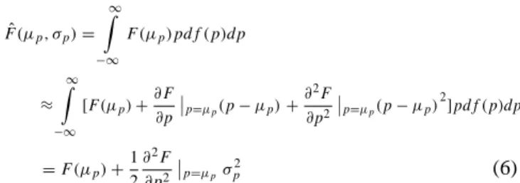
ˆ F (µp, σp) = ∞ Z −∞ F (µp)pdf (p)dp ≈ ∞ Z −∞ [F (µp) + ∂F ∂p  p=µp(p − µp) + ∂2_F ∂p2  p=µp(p − µp) 2 ]pdf (p)dp =F (µp) + 1 2 ∂2F ∂p2  p=µpσ 2 p (6)

(e.g. Papoulis, 1991), where pdf (p) is the probability den-sity function of p (in this case it is the normal distribution N (µp, σp)), and∂F_∂p  p=µp and ∂2_F ∂p2 

p=µp are first and

sec-ond derivatives of F with respect to the land surface param-eter p. As the first moment is approximated in second order accuracy, the approach is referred to as Second-Order-First-Moment propagation (SOFM).

The sensitivities are obtained analytically, as the SVAT-model is programmed in Mathematica, which allows alge-braic computation of derivatives, even for complex equations as it is in case of the numerical solution of the surface energy equations and all equations hereafter.

The effective parameter peffis based on the solution of

F (µp) + 1 2 ∂2F ∂p2  p=µp σ 2 p ! = F (peff) (7)

which requires determining the root of F (µp) + 1 2 ∂2F ∂p2  p=µp σ 2 p−F (peff) =0 (8)

H. Kunstmann: Upscaling of land-surface parameters through direct moment propagation 129

Figures

300 Sensible Heat Flux

Time [h] SH F [ W m -2 ] simulated observed 180 200 220 240 260 280 300 320 0 100 200 300 400 500

600 Latent Heat Flux

Time [h] LH F [ W m -2] simulated observed

Figure 1: Validation of SVAT-model: comparison between modelled and simulated sensible heat

fluxes (a, left) and latent heat fluxes (b, right)

Fig. 1. Validation of SVAT-model: comparison between modelled and simulated sensible heat fluxes (a, left) and latent heat fluxes (b, right).

1 p • • • n p

Subgrid scale fluxes: Fi (pi) _{Grid scale fluxes: F(}

eff

p )

Figure 2: Schematic presentation of definition of effective parameter peff and aggregation of heat

fluxes (adapted from Intsiful, 2004).

Subgrid scale Grid scale

Land surface parameters pi (i=1,..,n) Effective parameter, peff

Upscaling Time (Minutes) 0 20 40 60 80 S ens ib le He at Fl ux ( w m -2) 0 100 200 300 400 500 H-2 H-1 H-3 Time (minutes) 0 20 40 60 80 S ens ib le He at Fl ux ( W m -2) 0 100 200 300 400 500 Effective H

Fig. 2. Schematic presentation of definition of effective parameter peffand aggregation of heat fluxes (adapted from Intsiful, 2004).

This is easily achieved by standard packages within Mathe-matica.

For every given set of mean µp and standard deviation

σpat subgrid scale, the solution of the root finding problem

(8) has to be solved. The effective parameter then finally is

mapped as a function of µpand σp:

130 H. Kunstmann: Upscaling of land-surface parameters through direct moment propagation 0 0.05 0.1 0.15 0.2 0.25 0.3 0.35 0.4 0.45 0.5 0.8 0.82 0.84 0.86 0.88 0.9 0.92 0.94 0.96 0.98 1 SOFM z0m_eff (120h) σz0m/µz0m z0 mef f / µz0 m µ_z0m=0.075 µ_z0m=0.15 µz0m=0.3 µz0m=0.6 µz0m=0.9

Figure 3: Upscaling relations for roughness length

z

(SOFM method)

0 0.05 0.1 0.15 0.2 0.25 0.3 0.35 0.4 0.45 0.5 0.8 0.82 0.84 0.86 0.88 0.9 0.92 0.94 0.96 0.98 1

Monte Carlo z0m_eff (120h, 25 Realizations)

σ_z0m/µ_z0m z0 mef f /µz0 m µz0m=0.075 µz0m=0.15 µ_z0m=0.3 µ_z0m=0.6 µz0m=0.9

Figure 4: Upscaling relations for roughness length

z

(Monte Carlo method, 25 realizations)

Fig. 3. Upscaling relations for roughness length z0 m (SOFM

method).

4 Results

The proposed new approach for upscaling of land surface parameters is demonstrated for the parameters a) roughness length, b) wilting point soil moisture, and c) minimal stom-ata resistance. For the objective function to be met at grid scale, λE (latent heat flux) was chosen for F in (4) till (8). The upscaling relations are visualised by plotting the nor-malised effective parameter (i.e. peff/µp) against the

coeffi-cient of variation (i.e. σp/µp) for different mean parameter

values µp. Figure 3 shows the derived upscaling relation for

roughness length z0 m. It is seen that with increasing subgrid

scale heterogeneity (i.e. coefficient of variation) the effective roughness length is decreasing. Figure 4 shows the results of a corresponding Monte Carlo simulation. In fact the two approaches yield comparable results. Only in case of larger coefficients of variation, the Monte Carlo simulation differs. Effective parameters must be independent of the driving meteorology. The central question is: what is the minimum duration (episode) such that the derived value for the effec-tive parameter converges and becomes independent as time proceeds. Figure 5 shows the dependency of the derived ef-fective roughness length in dependence of simulation time. After around 80 h the derived effective value converges. It is therefore concluded that 120 h simulation time is sufficient for deriving effective land surface parameters in this study. It must be noted, however, that the effective parameters may still depend on regional climatology and the season of the year. A further investigation in this direction, however, is out of the scope of this study.

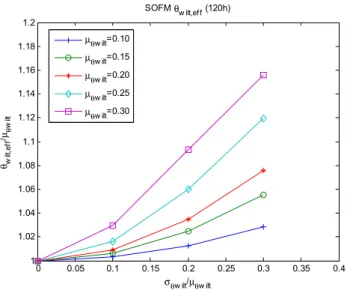
Figure 6 shows the upscaling relations in case of wilting point soil moisture θwilt. Contrary to the case of roughness

length, effective values increase with increasing coefficient of variation.

Figure 7 shows the upscaling relations for the vegetation type dependent minimum stomatal resistance Rcmin. The

0 0.05 0.1 0.15 0.2 0.25 0.3 0.35 0.4 0.45 0.5 0.8 0.82 0.84 0.86 0.88 0.9 0.92 0.94 0.96 0.98 1 SOFM z0m_eff (120h) σz0m/µz0m z0 mef f /µz0 m µ_z0m=0.075 µz0m=0.15 µz0m=0.3 µz0m=0.6 µz0m=0.9

Figure 3: Upscaling relations for roughness length

z

(SOFM method)

0 0.05 0.1 0.15 0.2 0.25 0.3 0.35 0.4 0.45 0.5 0.8 0.82 0.84 0.86 0.88 0.9 0.92 0.94 0.96 0.98 1

Monte Carlo z0m_eff (120h, 25 Realizations)

σz0m/µz0m z0 mef f /µz0 m µz0m=0.075 µz0m=0.15 µz0m=0.3 µz0m=0.6 µz0m=0.9

Figure 4: Upscaling relations for roughness length

z

(Monte Carlo method, 25 realizations)

SOFM z0m_eff/µzeff

SVAT Simulation Time [h]

z0 mef f /µze ff µ=0.04, σ=0.02 µ=0.04, σ=0.03 µ=0.04,σ=0.4 µ=0.075, σ=0.02 µ=0.075, σ=0.03 µ=0.75,_σ=0.4 µ=0.15, σ=0.02 µ=0.15, σ=0.03 µ=0.15,σ=0.4

Figure 5: Dependency of derived effective parameter on simulation time in case of roughness

length

z

: convergence after 60-80 h.

0 0.05 0.1 0.15 0.2 0.25 0.3 0.35 0.4 1 1.02 1.04 1.06 1.08 1.1 1.12 1.14 1.16 1.18 1.2 SOFM θ_{w ilt,eff} (120h) σ_θw ilt/µθw ilt θwilt,e ff /µθ w ilt µ_θw ilt=0.10 µ_θw ilt=0.15 µ_{θw ilt}=0.20 µ_θw ilt=0.25 µ_θw ilt=0.30

Figure 6: Upscaling relations for wilting point soil moisture

θ

(SOFM method)

Fig. 5. Dependency of derived effective parameter on simulation

time in case of roughness length z0 m: convergence after 60–80 h.

general shape of the scaling laws is similar to the case of roughness length.

5 Summary and conclusion

A new approach for the derivation of effective land surface parameters was presented. It was shown that the methodol-ogy yields results that are in excellent agreement with corre-sponding Monte Carlo results. The SOFM approach, how-ever, is much less computational demanding than the Monte Carlo approach. This is also due to the fact that the pro-gramming environment (Mathematica) chosen for this study allows the computationally efficient algebraic calculation of derivatives.

H. Kunstmann: Upscaling of land-surface parameters through direct moment propagation 131 0 20 40 60 80 100 120 140 160 180 200 0.8 0.82 0.84 0.86 0.88 0.9 0.92 0.94 0.96 0.98 1

SOFM z0m_eff/µzeff

SVAT Simulation Time [h]

z0 mef f /µze ff µ=0.04, σ=0.02 µ=0.04, σ=0.03 µ=0.04,σ=0.4 µ=0.075, _σ=0.02 µ=0.075, σ=0.03 µ=0.75,σ=0.4 µ=0.15, σ=0.02 µ=0.15, σ=0.03 µ=0.15,σ=0.4

Figure 5: Dependency of derived effective parameter on simulation time in case of roughness

length

z

: convergence after 60-80 h.

0 0.05 0.1 0.15 0.2 0.25 0.3 0.35 0.4 1 1.02 1.04 1.06 1.08 1.1 1.12 1.14 1.16 1.18 1.2 SOFM θ_{w ilt,eff} (120h) σ_θw ilt/µθw ilt θwilt,e ff /µθ w ilt µ_θw ilt=0.10 µ_θw ilt=0.15 µ_{θw ilt}=0.20 µ_{θw ilt}=0.25 µ_θw ilt=0.30

Figure 6: Upscaling relations for wilting point soil moisture

θ

(SOFM method)

Figure 7: Upscaling relations for minimum stomatal resistance Rc

(SOFM method)

0 0.05 0.1 0.15 0.2 0.25 0.3 0.35 0.4 0.9 0.91 0.92 0.93 0.94 0.95 0.96 0.97 0.98 0.99 1

SOFM rcmin_eff (120h)

σrcmin/µrcmin rc m inef f /µrc m in µrcmin=10.0 µrcmin=20.0 µrcmin=30.0 µrcmin=40.0 µrcmin=50.0 µrcmin=60.0

Fig. 7. Upscaling relations for minimum stomatal resistance Rcmin

(SOFM method).

Compared to other upscaling methods (e.g. Hu et al., 1999), the proposed methodology is independent of driving meteorology. It is concluded that the methodology proposed can also be advantageously applied in other areas, such as hydrogeology for example.

Acknowledgements. This work was performed within the

GLOWA-Volta project (http://www.glowa-volta.de) funded by the Germany Ministry of Education and Science (BMBF). The financial support is gratefully acknowledged.

Edited by: P. Krause, K. Bongartz, and W.-A. Fl¨ugel Reviewed by: anonymous referees

References

Ek, M. and Mahrt, L.: OSU 1-D PBL Model User’s Guide Version 1.0.4, Department of atmospheric Sciences, Oregon State Uni-versity, 1991.

Chen, F. and Dudhia, J.: Coupling an Advanced

Land-Surface/Hydrology Model with the Penn State/NCAR MM5 Modeling System, Part I: Model Implementation and Sensitiv-ity, Monthly Weather Review, 129, 569–585, 2001.

Grell, G., Dudhia, J., and Stauffer, D.: A Description of the Fifth-Generation Penn State/NCAR Mesoscale Model (MM5), NCAR Technical Note, NCAR/TN-398+STR, pp. 117, 1994.

Hu, Y., Islam, Y., and Jiang, L.: Approaches for aggregating hetero-geneous surface parameters and fluxes for mesoscale and climate models, Boundary Layer Meteorology, 93, 313–336, 1999. Intsiful, J.: Upscaling of Land Surface Parameters through Inverse

SVAT modelling, PhD at Bonn University, published in Ecol-ogy and Development Series, No. 20, Cuvillier Verlag G¨ottingen, ISBN 3-86537-174-4, 2004.

Papoulis, A.: Probability, Random Variables and Stochastic Pro-cesses, McGraw Hill, 1991.