HAL Id: hal-00296754
https://hal.archives-ouvertes.fr/hal-00296754
Submitted on 17 Jun 2003
HAL is a multi-disciplinary open access
archive for the deposit and dissemination of
sci-entific research documents, whether they are
pub-lished or not. The documents may come from
teaching and research institutions in France or
abroad, or from public or private research centers.
L’archive ouverte pluridisciplinaire HAL, est
destinée au dépôt et à la diffusion de documents
scientifiques de niveau recherche, publiés ou non,
émanant des établissements d’enseignement et de
recherche français ou étrangers, des laboratoires
publics ou privés.
Error assessment of GOCE SGG data using along track
interpolation
J. Bouman, R. Koop
To cite this version:
J. Bouman, R. Koop. Error assessment of GOCE SGG data using along track interpolation. Advances
in Geosciences, European Geosciences Union, 2003, 1, pp.27-32. �hal-00296754�
c
European Geosciences Union 2003
Advances in
Geosciences
Error assessment of GOCE SGG data using along track
interpolation
J. Bouman1and R. Koop1
1SRON National Institute for Space Research, Utrecht, The Netherlands
Abstract. GOCE will be the first satellite gravity mission
measuring gravity gradients in space using a dedicated in-strument called a gradiometer. High resolution gravity field recovery will be possible from these gradients. Such a re-covery requires a proper description of the gravity gradient errors, where the a priori error model is for example based on end-to-end instrument simulations. One way to test the error model against real data, i.e. to see if the a priori model really describes the actual error, is to compare along track interpo-lated gradients with the measured gradients. The difference between the interpolated and measured gravity gradients is caused by, among others, the interpolation error and the mea-surement errors. The idea is that if the interpolation error is small enough, then the differences should be predicted rea-sonably well by the error model. This paper discusses a sim-ulation study where the gravity gradient errors are generated with an end-to-end instrument simulator. The measurement error will be compared with the interpolation error and we will assess the latter as a function of the sampling interval.
1 Introduction
The main goal of the GOCE mission (expected to be launched early 2006) is to provide unique models of the Earth’s gravity field and the geoid, on a global scale with high spatial resolution and to very high accuracy (ESA, 1999). To this end, GOCE will be equipped with a GPS receiver for high-low satellite-to-satellite tracking (SST-hl) observa-tions, and with a gradiometer for observation of the gravity gradients (SGG). The gradiometer consists of six 3-axes ac-celerometers mounted in pairs along three orthogonal arms. From the readings of each pair of accelerometers the so-called common mode (CM) and differential mode (DM) sig-nals are derived. The CM observations are used to obtain in-formation about the linear accelerations and are input to the drag free control system. The measurements of the CM are Correspondence to: J. Bouman ([email protected])
also needed for accurate separation of the non-conservative and conservative forces and are therefore important for the long wavelength gravity field recovery from SST measure-ments. The DM observations are used to derive the required gravity gradients. The accelerometers and the gradiometer are designed such as to give the highest achievable precision in the measurement bandwidth (MBW) between 5 and 100 mHz. For the diagonal gravity gradients in a Local Orbital Reference Frame (LORF, X-axis in the velocity direction, the Z-axis approximately radially outward and the Y -axis complements the right-handed frame) this precision will not exceed 4 mE/
√
Hz (1 E = 10−9 s−2) in the MBW (Cesare, 2002).
The observations will be contaminated with stochastic and systematic errors. For the GOCE gradiometer, systematic er-rors typically are due to instrument imperfections like mis-alignments of the accelerometers, scale factor mismatches etc. The CM and DM couplings, which are the result of such instrument imperfections, can be determined to an accuracy level of 10−2−10−4prior to the mission by the so-called pre-flight calibration on ground using a test bench (Cesare, 2002). In orbit, a so-called internal calibration procedure will be used (ESA, 1999), by which the CM and DM cou-plings can be determined to an accuracy level at which their effect on the gradients in the MBW stays below the required 4 mE/
√
Hz. The values of the calibration parameters (ele-ments of the calibration matrix) are measured by putting a known acceleration signal on the gradiometer in orbit using the thrusters. After this procedure, the CM and DM read-outs of the gradiometer are corrected using the measured calibra-tion parameters.
The gravity gradients are derived from the internally cali-brated DM accelerations. The internal calibration, however, is not sensitive to all instrument imperfections. For example, the true locations of the six accelerometers may differ from their nominal positions. This accelerometer mis-positioning as well as the read-out bias, for example, can not be ac-counted for. Therefore, in order to possibly correct for re-maining errors after internal calibration, a third calibration
28 J. Bouman and R. Koop: Error assessment of GOCE SGG data step is required, which is called external calibration (or
abso-lute calibration). It is performed during or after the mission and typically makes use of external gravity data (Arabelos and Tscherning, 1998; Koop et al., 2002).
Along with the external calibration of the observations, their error needs to be assessed. For this purpose, we could use either external data, such as terrestrial gravity data, or use the GOCE data themselves and perform an internal as-sessment. In view of the very high accuracy of GOCE in the MBW, it will be difficult to assess the gravity gradient errors in the MBW with the former method. We therefore focus on internal error assessment. Specifically, the pros and cons of along track data interpolation are studied. Albertella et al. (2000b) use along track interpolation for outlier detec-tion, while the use of cross-overs and repeat tracks for error assessment is studied by Albertella et al. (2000a) and Koop et al. (2002), respectively.
The along track interpolation and error assessment is in-troduced in Sect. 2. The interpolation error is discussed in Sect. 3 for several cases, while the error assessment itself is discussed in Sect. 4.
2 Along track interpolation
GOCE will deliver time series of gravity gradients along its orbit. A subset of the time series may be used to interpolate at time t = i. The difference between the interpolated ˆy(i) and the measured y(i) is due to, among others, the interpolation error and the measurement errors. If the interpolation error is small enough then the above differences could be used for error assessment. The general interpolation model as well as the error assessment are discussed in more detail in this section.
2.1 Model of condition equations The model of condition equations is
BTE{y} = 0; D{y} = Qy (1)
with least squares errors ˆ
e = QyB(BTQyB)−1BTy. (2)
The observations y are the gravity gradients TXX, TYY, TZZ
in the LORF. The anomalous gravity gradients Tjj, with
j = X, Y, Z, are obtained by taking the difference between the measured gradients and some reference model values. The model BT depends on the specific interpolation method, but for local interpolation methods BT will be sparse. The central idea is: interpolate one or more observations from other observations and compare the interpolated values with the original ones. The error variance-covariance matrix Qy
is full in general. Due to the coloured noise behaviour of the gradiometer, the gravity gradient errors will be correlated in time.
2.2 Overall model test
An unbiased estimate of the variance of unit weight is ˆ
σ2= eˆ
TQ
y−1eˆ
b (3)
with b the rank of B, that is, the number of independent con-dition equations. Thus ˆσ2depends on the a priori error ma-trix Qyand the a posteriori error ˆe. In practice one could use
Eq. (3) to test whether one a priori error model is to be pre-ferred over the other. The closer ˆσ2is to 1, the more likely it is that the corresponding a priori model Qydescribes the
er-rors well assuming that outliers have been removed and that the variance of unit weight is 1.
The distribution of ˆσ2 under the null hypothesis H0(i.e.
the a priori error model is correct) is given as
H0: ˆσ2∼F (b, ∞,0) (4)
that is a central F distribution. The a priori error model will be rejected if ˆσ2 > kα, that is, if the a posteriori variance
of unit weight is larger than a critical value with significance level α. For example F0.05(60, ∞, 0) = 1.4, which means
that for 60 conditions equations the a priori error model will be rejected if the a posteriori variance of unit weight is larger than 1.4. In approximately 5% of the cases the null hypoth-esis will be rejected although the a priori error model is cor-rect.
2.3 Comparison with other methods
The advantage of along track interpolation for error assess-ment is that it can be started right after the first measureassess-ments are available (provided that the on board navigation solution is accurate enough). There are no conditions on the repeat of the orbit or on the cross-overs. Interpolation methods typ-ically use local data, which means that this method may be suited to assess the error especially for high frequencies, that is, near or inside the MBW. A disadvantage may be that sys-tematic, long wavelength errors will not be visible using local interpolation methods. Hence, long wavelength errors could go undetected. This problem may be overcome using global interpolation methods, however, this may increase the inter-polation error.
Koop et al. (2002) discuss the use of repeat tracks for in-ternal error assessment, while Albertella et al. (2000a) use cross-overs. Both methods are in the form of model (1). Cross-overs are not suited to test the TXX and TYY errors
due to large measurement errors in the off-diagonal gravity gradients, which are needed to transform the ascending and descending measurements to a common frame. The radial gravity gradient TZZ, however, can be tested. Especially, the
cross-overs after one or a few revolutions can be used, while the cross-overs further apart in time are less useful. The ra-dial orbit variations at cross-overs tend to increase in time, which affects the comparisons (Albertella et al., 2000a). In addition, cross-overs are less dense than the along track sam-pling, so the high frequency errors can not be assessed.
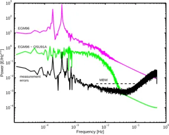
10−4 10−3 10−2 10−1 100 10−4 10−3 10−2 10−1 100 101 102 103 Frequency [Hz] Power [E/Hz 1/2 ] MBW EGM96 EGM96 − OSU91A measurement errors
Fig. 1. Spectral densities of the TYYsignal and measurement errors.
In principle, repeat tracks can be used to test the whole spectral range, which is a clear advantage. The method, how-ever, heavily relies on a close repeat of the orbit after some time. Specifically the radial distance, that is, the distance in the Z-direction, between repeat tracks has to be small, and therefore Koop et al. (2002) consider a so-called frozen orbit, which minimizes the radial orbit variations. It is, however, unlikely that the GOCE orbit will be a frozen orbit and a re-peat is even avoided as much as possible within two months to get a dense spatial cross track coverage, (see ESA, 1999). These three internal error assessment methods (along track interpolation, cross-overs, repeat tracks) are therefore more or less complementary.
3 Interpolation error
The along track interpolation errors should be small enough compared to the measurement errors. This is a necessary condition for the along track interpolation method to be use-ful. Two simple interpolation methods are tested: linear in-terpolation and Overhauser splines (Overhauser, 1968). Al-though the interpolation methods do not require so, it is as-sumed for simplicity that the along track sampling is regular. In practice this will probably be realized for many time in-tervals during the GOCE mission and it is certainly true for our simulations. Results for linear interpolation will not be shown. Despite the interplation error is small compared to the measurement error for this method, Overhauser splines yield a factor of two smaller interpolation errors. The former method will therefore not be used in this paper.
True gravity gradients in the LORF were generated using the global gravity field model EGM96. Anomalous grav-ity gradients were computed by subtracting reference gravgrav-ity gradients computed with OSU91A. These anomalous grav-ity gradients will be used in the interpolation error test. First, no errors are added to the measurements and the orbit is as-sumed to be known. Then the residuals BTy 6= 0 are entirely
Table 1. RMS of gravity gradient measurement errors and
Over-hauser spline interpolation errors in [mE]
TXX TYY TZZ
interpolation errors 0.04 0.01 0.04 measurement errors 8.2 9.7 8.5
due to the interpolation. The gravity gradient data sets have a length of 1 day and the sampling interval is 1 s.
Overhauser splines are cubic splines that are one time continuously differentiable at the data points (Overhauser, 1968). For equidistant data points the condition equations take the form
y(i) = 7
12[y(i − k) + y(i + k)] +
− 1
12[y(i − 2k) + y(i + 2k)] (5)
where k = 1 or 2 or . . .. If k = 1 then neighbouring points are used for the interpolation, if k = 2 then every second point is used, etc. Suppose k = 1 and there are m measure-ments, then i may take the values 3, . . . , m − 2.
Table 1 lists the Root Mean Square (RMS) of the gravity gradient measurement errors as well as the RMS of interpola-tion errors due to interpolainterpola-tion with Overhauser splines. The former errors are obtained after external calibration of the original gravity gradients as described in Koop et al. (2002). The errors due to interpolation are therefore two to three or-ders smaller than the measurement errors, with the TXXand
TZZinterpolation errors larger than the TYY errors.
The spectral densities of the full and residual signal as well as the measurement errors are shown, for TYY, in Fig. 1,
whereas the interpolation errors are shown in Fig. 2. The er-ror due to interpolation is below the measurement erer-ror over the entire spectrum. Since the interpolation is local, the inter-polation error is small for the low frequencies. In the MBW the interpolation error is clearly correlated with the residual signal, that is, with the gravity gradient anomalies (EGM96 – OSU91A). It should be noted that degree 360 is the max-imum spherical harmonic degree of the gravity field models in the simulations. At the Earth’s surface this corresponds to a resolution of roughly 55 km, which is a distance the GOCE satellite will travel in 7 s, given its along track velocity of 7.8 km/s. Consequently, the true gravity signal is probably not well presented in our simulations for frequencies larger than 7×10⁻²Hz or so. Above the MBW, > 0.1 Hz, the inter-polation error increases. Since there is practically no resid-ual signal in the current simulation above the MBW, this may be caused by round-off errors. The small peak at 0.1 Hz is not well understood. The interpolation error in the MBW is slightly larger for TXXand TZZ, although still well below the
measurement error.
In general the interpolation error increases for increasing sample distance. This is shown in Fig. 2 for the time series
30 J. Bouman and R. Koop: Error assessment of GOCE SGG data 10−5 10−4 10−3 10−2 10−1 100 10−7 10−6 10−5 10−4 10−3 10−2 10−1 100 Frequency [Hz] Power [E/Hz 1/2 ] MBW measurement errors interpolation error 4 s sampling interpolation error 1 s sampling
Fig. 2. Spectral densities of measurement and interpolation errors
for TYY.
resampled such that time distance between successive obser-vations is 4 s. The interpolation error is smaller than the measurement error for samples up to 2 s distance for all fre-quencies (not shown). The interpolation error is larger than the measurement error in the MBW for TXX and TZZ for a
sample distance of 4 s, whereas the interpolation error for TYY is still below the measurement error for all frequencies
at this sampling interval, as is shown in Fig. 2.
So far, overlapping intervals have been used, that is, ob-servations 1, 2, 4, and 5 are used to predict 3, then 2, 3, 5, and 6 are used to predict 4, etc. One could also use non-overlapping intervals, that is, use observations 1, 2, 4, 5 to predict 3, then use 6, 7, 9, 10 to predict 8, etc. Since the interpolation error is a systematic error (it depends on the signal), the error decreases slightly for the non-overlapping case: there are 5 times less condition equations (results are not shown).
4 Statistical test results
In the previous section it was shown that for a 1 s sample interval the interpolation error can be neglected compared to the measurement error. The model of condition Eqs. (1) holds, and the appearance of BT depends on whether we use 1 s shifts or 2 s shifts etc. between successive condition equa-tions. The error assessment requires that an a priori error model Qyis available. Our first aim is therefore to compute
such an error model, and to study its characteristics.
In general, the error variance-covariance matrix is full. The errors on the GOCE gravity gradients are coloured, that is, the error is small in the MBW and increases outside the MBW, see also Fig. 1. This yields along track error correla-tion. If the full data period is considered (1 day) then error correlations exist that can not be neglected. Especially for TYY and TZZthis is true because 1, 2, etc. cpr (cycles per
rev-olution) errors are present, see Figs. 2 and 3. These errors
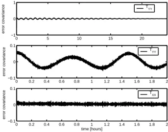
0 5 10 15 20 −1 0 1 error covariance 0 0.2 0.4 0.6 0.8 1 1.2 1.4 1.6 1.8 2 −0.1 0 0.1 error covariance 0 0.2 0.4 0.6 0.8 1 1.2 1.4 1.6 1.8 2 −0.1 0 0.1 time [hours] error covariance TYY TXX T YY
Fig. 3. Gravity gradient error covariances for 1 day. Top panel: TYY
1 day; middle panel: TYY zoom in on first 2 h; bottom panel: TXX
zoom in on first 2 h.
are much smaller for TXX, which results in much smaller
er-ror correlations. Shown in the top panel of Fig. 3 are the true TYY error covariances for the total time series of 1 day, scaled
with the variance at t = 0. Hence, at t = 0 the error covari-ance is 1, but this is hard to distinguish in the present graph. Zooming in on the first 2 h of the error covariances shows strong correlations (middle panel). The error covariances of TZZare similar to those of TYY. Because external calibration
significantly reduced the TXX errors at 1 and 2 cpr, the
cor-relation is less for longer time intervals (see Fig. 3, bottom panel).
The overall model test requires the inversion of the (full) error matrix Qy, Eq. (3). Limiting our test to time
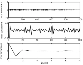
win-dows of 1000 s, for example, would allow straightforward computations. A disadvantage is that the test of the valid-ity of a priori error models becomes limited. However, the most interesting part of GOCE, the MBW, is contained in these windows and the along track interpolation, which we study here, is not sensitive to longer wavelengths. Figure 4 shows the TYY error covariances, averaged over 86 windows
of 1000 s. Before the error covariance of each window is computed, the mean was subtracted, which in effect removes part of the long wavelength errors. Therefore, the average er-ror covariance for the full 1000 s period appears to be noisy (top panel). Zooming in, however, on the first 100 s shows that correlations up to 10–15% still remain (Fig. 4, middle panel). The correlation is strongest for the first 2–3 s (bot-tom panel). The TXX and TZZ error covariances for 1000 s
show similar behaviour to those of TYY.
The averaged empirical error covariance functions for the 1000 s windows have been used to create three a priori error matrices Qy (one for each studied gravity gradient).
Since these matrices are based on the true (simulated) er-rors, one should expect that the a priori error model will be accepted for nearly all error assessment windows. Two
ex-0 200 400 600 800 1000 −1 0 1 error covariance 0 20 40 60 80 100 −0.2 0 0.2 error covariance 0 2 4 6 8 10 −1 0 1 time [s] error covariance
Fig. 4. TYY error covariances averaged over 1000 s windows. Top panel: full 1000 s period; middle panel: zoom in on first 100 s; bottom panel: zoom in on first 10 s.
0 10 20 30 40 50 60 70 80 90 1 1.1 1.2 1.3 1.4 1.5 Rejected intervals (4.3 %) Interval Test value xx (5 s): 3 yy (5 s): 5 zz (5 s): 2 xx (2 s): 5 yy (2 s): 4 zz (2 s): 3
Fig. 5. Rejected ˆσ2values. In total 22 out of 6 ∗ 86 = 516 values are rejected.
amples are shown in Fig. 5 and Tables 2 and 3. The trian-gles denote the rejected test values for interpolation in win-dows of 1000 s length, 1 s sampling and 5 s shifts between condition equations. Hence there are roughly 200 condi-tion equacondi-tions: F0.05(200, ∞, 0) ≈ 1.2. The circles
de-note the rejected test values for interpolation in windows of 1000 s length, 1 s sampling and 2 s shifts between condition equations. Hence there are roughly 500 condition equations: F0.05(500, ∞, 0) ≈ 1.1. In total 4.3% of the a posteriori
variances are too large and rejected, which is a satisfactory result.
As the bottom panel of Fig. 4 suggests, the full error matrix
Qy can be approximated by a sparse matrix (band matrix).
Considering the error covariance functions, we use the first 4 points of the covariance functions. The number of rejected a
Table 2. Average a posteriori variance of unit weight and F -test
results. Error assessment window is 1000 s (86 windows), sampling interval is 1 s, interpolation shift is 2 s
Qy full band diag Qyof TXX
ˆ
σ2 rej. σˆ2 rej. σˆ2 rej. σˆ2 rej.
TXX 1.00 5 1.00 5 1.80 86 1.00 5
TYY 1.00 4 1.00 5 1.76 86 1.35 86
TZZ 1.00 3 1.00 5 1.74 86 1.00 5
Table 3. Average a posteriori variance of unit weight and F -test
results. Error assessment window is 1000 s (86 windows), sampling interval is 1 s, interpolation shift is 5 s
Qy full band Qyof TXX
ˆ
σ2 rej. σˆ2 rej. σˆ2 rej.
TXX 0.99 3 1.00 3 0.99 3
TYY 1.00 5 1.01 4 1.35 77
TZZ 1.01 2 1.01 2 1.01 3
posteriori variances increases slightly: 4.7% is rejected. Ne-glecting all correlations and using the variances only does not give satisfactory results. The a priori error model is rejected for all error assessment windows. See Tables 2 and 3.
If the a priori error matrix Qyof TXXis used for the other
two gradients, then it is rejected for (nearly) all TYY
win-dows, whereas the TZZ results stay the same, see Tables 2
and 3. This is a consequence of the fact that, in our simu-lation for short time intervals, the TXXerror covariances are
almost equal to those of TZZ. The differences with the TYY
error are somewhat larger for short time intervals. The error assessment using along track interpolation is therefore rather sensitive to the correct error model. Or at least, sensitive to too optimistic error models. If we use a pessimistic error model, for example multiply the error model of TZZ with a
factor of 1.5, then the a priori error model is accepted for all windows. However, the average a posteriori variance of unit weight is ˆσ2 = 1/1.5 for 86 windows. It may therefore be necessary to apply a double-sided statistical test instead of one-sided test as we do now.
Finally, a 1 s sampling and 1 s condition equation shift yields a badly conditioned BTQyB matrix. Consequently,
the test results are unreliable. This may be a consequence of too much correlation or may have some other cause, yet unresolved.
5 Conclusions and discussion
Along track interpolation is well suited to test the a priori error model for GOCE SGG observations. This method is complementary to other methods of error assessment such as the use of repeat tracks and cross-overs. The major advantage
32 J. Bouman and R. Koop: Error assessment of GOCE SGG data of along track interpolation is that it is independent of the
repeat conditions of the satellite ground track and that it may be applied real time. Thus, in the context of quick-look data quality assessment, this tool is a major candidate for real time monitoring of the instrument in flight.
The assumptions underlying the current simulation study are that no outliers are present and that the orbit naviga-tion solunaviga-tion is accurate enough. In reality, outliers will be present, and they have to be dealt with before the interpola-tion error assessment is performed. Outliers can be removed on basis of an a priori error model. Hence, a kind of iter-ative procedure comes to mind. Further, orbit uncertainties in the navigation solution contribute to the interpolation er-ror, since the method assumes known locations of the mea-surements, and the observations are reduced w.r.t. an a priori gravity model. It has to be assessed what the upper limit is for the accuracy of the navigation solution for our method to work properly.
The interpolation error is very small compared to measure-ment error for 1 s sampling. For the TXX and TZZ
gradi-ents the interpolation error is larger than for the TYY
gradi-ent. In our simulations we used a reference model and sub-tracted it from the simulated gravity gradients, which gives residual gravity gradients. Since the maximum spherical har-monic degree is 360 in these simulations, there is concern that the residual signal is unrealistic for high frequencies. Or, in other words, the residual gravity gradient signal may be much larger for high frequencies when reference gravity gradients are subtracted from true, measured gradients. How this influences the interpolation needs to be studied.
Error assessment windows are limited to 1000 s or so due to computer restrictions. An advantage is that the error corre-lation is largest for the first few seconds, so that a priori error matrix Qymay be approximated by a band matrix. In
addi-tion, the interpolation methods are local and therefore proba-bly not too sensitive to long wavelength errors. Disadvantage is that not the entire spectrum can be tested. Importantly, the entire GOCE MBW is contained in our test.
We accept the a priori error model if the F -test does not re-ject too many a posteriori variances of unit weight (based on a chosen signifigance level) and the average a posteriori vari-ance of unit weight has to be “close” to one. In this way, we can use this method in reality to test any choice of an a priori error model to find the best model for the real observations. In order to prevent a false acceptance of a too pessimistic a
priori model, our one-sided statistical test should be replaced by a double-sided test.
If the a priori error model is rejected then either the model is wrong indeed or the interpolation error is too large. We may then increase the sample interval, a factor of two for example. If the statisical test yields the same results then the a priori model is false. If more points are rejected then at least the interpolation error in the latter test is too large. We can not say more about the former test. We therefore need information on the interpolation error beforehand.
Acknowledgements. The satellite orbit and the EGM96 gravity
gra-dients were provided by Karl Heinz Ilk as part of simulation sce-narios of Special Commission 7 in cooperation with Special Study Group 2.193 of the International Association of Geodesy, which is appreciated. Volker Hannen computed the simulated gravity gradi-ent errors, which is appreciated as well. We also acknowledge the use ofnewmat, a C++ matrix library developed by Robert Davies. The software can be downloaded from the Internet, and this matrix library supported part of the computations.
References
Albertella, A., Migliaccio, F., Sans`o, F., and Tscherning, C.: The space-wise approach - overall scientific data strategy, in: From E¨otv¨os to mGal, Final Report, (Ed) S¨unkel, H., ESA/ESTEC contract no. 13392/98/NL/GD, 2000a.
Albertella, A., Migliaccio, F., Sans`o, F., and Tscherning, C.: Scien-tific data production quality assessment using local space-wise pre-processing, in: From E¨otv¨os to mGal, Final Report, (Ed) S¨unkel, H., ESA/ESTEC contract no. 13392/98/NL/GD, 2000b. Arabelos, D. and Tscherning, C.: Calibration of satellite
gradiome-ter data aided by ground gravity data, Journal of Geodesy, 72, 617–625, 1998.
Cesare, S.: Performance requirements and budgets for the gradio-metric mission, Issue 2 GO-TN-AI-0027, Preliminary Design Review, Alenia, 2002.
ESA: Gravity Field and Steady-State Ocean Circulation Mission, Reports for mission selection; the four candidate earth explorer core missions, ESA SP-1233(1), 1999.
Koop, R., Bouman, J., Schrama, E., and Visser, P.: Calibration and error assessment of GOCE data, in: Vistas for Geodesy in the New Millenium, (Eds) ´Ad´am, J. and Schwarz, K.-P., vol. 125 of International Association of Geodesy Symposia, pp. 167–174, Springer, 2002.
Overhauser, A.: Analytic definition of curves and surfaces by parabolic blending, Techn. Report No. SL68-40, Scientific Re-search Staff Publication, Ford Motor Company, Detroit, 1968.