HAL Id: hal-03121187
https://hal.archives-ouvertes.fr/hal-03121187
Submitted on 26 Jan 2021HAL is a multi-disciplinary open access archive for the deposit and dissemination of sci-entific research documents, whether they are pub-lished or not. The documents may come from teaching and research institutions in France or abroad, or from public or private research centers.
L’archive ouverte pluridisciplinaire HAL, est destinée au dépôt et à la diffusion de documents scientifiques de niveau recherche, publiés ou non, émanant des établissements d’enseignement et de recherche français ou étrangers, des laboratoires publics ou privés.
Estimating time-varying stage-discharge relations in
rivers with aquatic vegetation
Emeline Perret, Jérôme Le Coz, Benjamin Renard
To cite this version:
Emeline Perret, Jérôme Le Coz, Benjamin Renard. Estimating time-varying stage-discharge relations in rivers with aquatic vegetation. River Flow 2020, Jul 2020, Delft, Netherlands. �hal-03121187�
1 INTRODUCTION
At hydrometric stations, streamflow records are generally computed using stage-discharge mod-els, also called rating curves. Hydrometric stations are commonly installed on river sections where it is possible to obtain a unique relation between the water level (stage) h and the dis-charge Q for a given time period. The standard form of the rating curve for a given hydraulic control (section or channel control) is a power equation (Le Coz et al., 2014):
𝑄 = 𝑎(ℎ − 𝑏)𝑐 (1)
where a = coefficient related to the type of control (=𝐵√𝑆0/𝑛 for a wide and rectangular channel
control, with B = channel width, S0 = channel slope and n = Manning friction coefficient), b = offset; and c = exponent related to the type of control (=5/3 in the case of a wide rectangular channel control). These parameters are estimated based on expert knowledge and using gaug-ings, which are occasional measurements of stage and discharge carried out at the studied sta-tion. This simple power equation is no longer suitable when the system is subject to instabilities that modify the hydraulic control. In practice, sudden (e.g. due to morphological evolution in-duced by a flood) or transient (e.g. due to the evolution of vegetation) rating changes can hap-pen (Mansanarez et al., 2019). Then, the discharge needs to be computed using h and other vari-ables (e.g. time-varying varivari-ables).
In this paper, we focus on stations affected by the presence of aquatic vegetation. Stage-discharge relations vary continuously in time due to the vegetation evolution. To our knowledge, no standardized methods nor convenient stage-discharge models exist to manage such transient changes. Some countries use manual adjustments to compensate for the effect of plants (e.g. the corTH method used by the French hydrometric services) but such procedure is subjective, labor-intensive and rather uncertain.
Estimating time-varying stage-discharge relations in rivers with
aquatic vegetation
E. Perret, J. Le Coz & B. Renard
INRAE, UR RiverLy, Lyon, France
ABSTRACT: Stage-discharge relations at hydrometric stations with aquatic vegetation vary continuously in time due to the vegetation evolution. Maintaining such rating curves for estab-lishing discharge time series is a challenge. Generally, the curves are adjusted manually as con-venient stage-discharge models are missing. To fill this gap, we developed a practical model that accounts for transient changes due to aquatic vegetation. It is restricted to hydraulic controls that can be described by the Manning-Strickler equation for wide rectangular channels. In most situations, aquatic plants induce changes in bed roughness and mainly affect flow resistance. Bed roughness is characterized using a time-varying Manning coefficient, estimated using a friction equation accounting for the vegetation development (growth and decay) and for the plant flexibility (bending). In this paper, we illustrate the need to take into account flow-induced plant bending in the friction equation even though vegetation development remains the main factor affecting the flow resistance.
From a physical point of view, the presence of vegetation essentially induces a resistance to water flow, just like the resistance due to bed material, bed forms, etc. (Coon, 1998, Green, 2005). All of these factors contribute to the total flow resistance, which can be expressed as a friction coefficient such as the Manning coefficient n. The impact of plants growing from the bank, which can obstruct the flow and reduce the wetted flow section, is generally assumed neg-ligible compared to the effect of plants on the flow resistance. This assumption can be arguable during some extreme flow events. Several decomposition methods for n have been proposed in the literature (Cowan, 1956, Morin et al., 2000). The expression of Morin et al. (2000) is chosen for this study in order to particularly focus on the vegetation effect on the flow:
𝑛2= 𝑛 𝑏 2+ 𝑛
𝑣
2 (2)
where n = total Manning coefficient, nb = Manning coefficient of the bed when there is no vege-tation; and nv = Manning coefficient related to additional friction due to plants. The resistance related to plants is the most likely to vary in time and one of the most difficult to estimate. In-deed, nv(t) depends on the type of plants, their spatial distribution, their density, their develop-ment, their relative submergence, their flexibility, etc. Few friction equations exist to compute
nv(t) in contrast to the numerous equations or look-up tables for nb (Meyer-Peter and Müller, 1948, Limerinos, 1970, Coon, 1998). Unfortunately, these friction equations related to vegeta-tion are either too simple to represent the effect of natural plants (see the analogy of the vertical rigid cylinder in Petryk and Bosmajian (1975) or in Pasche and Rouvé (1985)) or too complex (Aberle and Järvelä, 2013) and require too much information to be used for operational purpos-es (e.g. such as plant elasticity, Leaf Area Index, plant growth rate depending on a range of ex-ternal factors such as the water temperature).
In this paper, we aim to better predict the stage-discharge relation at stations affected by aquatic vegetation. We develop a new rating curve model that varies in time, based on the standard power model and on a time-varying friction equation. The model intends to be used for operational purposes, using information that can be easily retrieved in the field. The model is tested on data from a French hydrometric station affected by aquatic vegetation. The objective is to show that the simple use of a time-varying friction coefficient in the model improves the dis-charge prediction in presence of plants. We also discuss the importance of the choice of the fric-tion equafric-tion. In particular, we emphasize the need to account for plant bending and not only for plant biomass evolution, even if the latter is the main factor influencing the flow resistance.
2 TIME-VARYING FRICTION EQUATION RELATED TO AQUATIC VEGETATION The new rating curve model is similar to the standard power equation (Eq. 1), except for the Manning friction coefficient n now varying in time because of the component nv(t) related to the vegetation (see Eq. 2). Our study is restricted to hydraulic controls that can be described by the Manning-Strickler equation for wide rectangular channels.
2.1 Simplified Järvelä (2004) equation
Friction equations were developed in specific conditions (i.e. emergent or submerged plants, flexible plant or not). In this study, we focus on aquatic plants (e.g. macrophytes) that are locat-ed in the main channel and submerglocat-ed (with low relative submergence). Most of the time, these plants are flexible. We also assume that their spatial distribution is homogeneous throughout the channel section. The friction equation of Järvelä (2004) was developed for evaluating the fric-tion coefficient related to those types of plants at the reach-scale:
𝑛𝑣2(𝑡) = 4𝐶𝐷𝜒𝐿𝐴𝐼(𝑡)[ℎ(𝑡)−𝑏]1/3 8𝑔 min (( 𝑈𝑚 𝑈𝜒) 𝜒 ; 1) (3)
where CDχ = drag coefficient related to the plants, LAI = Leaf Area Index, g = gravity accelera-tion, χ = reconfiguration coefficient specific to the plant species (e.g. χ = 0 for rigid plants and χ
= -1 for leafy flexible plants), Um = mean velocity; and Uχ = the lowest velocity used during the experimental determination of χ. The plant can bend only when the mean velocity exceeds a
We add this condition to the original Järvelä (2004) equation using the min() function. The Järvelä (2004) equation can be seen as a combination of two main functions that account for two main factors: the plant development (using the LAI) and the plant capacity to bend and align un-der the action of flow (using the mean velocity). Plants bend to limit their frontal areas impacted by the flow, which leads to reduced bed roughness induced by the vegetation when flow veloci-ty increases. In practice, the LAI data are scarce and no biomass measurements are generally performed at hydrometric stations. Equation 3 is thus too complex for our study. We propose a new friction equation, which is a simplification of the Järvelä (2004) equation:
𝑛𝑣2(𝑡) = 𝐺(𝑡)[ℎ(𝑡)−𝑏]1/3 8𝑔 min (( 𝑈𝑚(𝑡) 𝑈𝜒 ) 𝜒 ; 1) (4)
G(t) = potential of hydraulic resistance due to the development of plants (growth and decay). It
is assumed that G(t) evolves similarly in shape as the plant biomass. G(t) is thus a proxy of the evolution of the plant biomass. It cannot be measured specifically, but can be modelled using models for biomass development.
2.2 Proxy of biomass evolution
We assume that the biomass (and consequently the proxy G(t)) is a function of time during the year (i.e. during the plant cycle of growth and decay). A bell-shaped model as presented in Fig-ure 1 is chosen for modeling G(t) (Yin et al., 2003):
𝐺(𝑡) = 𝐺𝑚𝑎𝑥( 𝑡−𝑡𝑏 𝑡𝑒−𝑡𝑏) 𝑡𝑒−𝑡𝑏 𝑡𝑒−𝑡𝑚 ⁄ (2𝑡𝑒−𝑡𝑚−𝑡 𝑡𝑒−𝑡𝑚 ) (5)
where Gmax = maximum plant proxy biomass, tb = beginning of plant growth, tm= time at which the growth rate is maximum; and te = end of plant growth and beginning of decay. Equation 5 is built such as no negative biomass is allowed. Equation 5 reflects the general trend of the bio-mass evolution, but does not take into account any external perturbations (e.g. flood, sudden drop in water temperature) that might induce some changes in the shape of the biomass evolu-tion. More complex models for the biomass evolution exist such as dynamic models depending on external factor (nutrient, light intensity, water temperature, etc.) (Lazár et al., 2016) but they require much more information not always available for operational purposes.
Figure 1. Shape of the model used for modelling the biomass proxy G(t).
2.3 Final friction equation
The final time-varying friction equation to include in the power equation (Eq.1 combined with Eq. 2) is the following:
𝑛𝑣2(𝑡) = 𝐺𝑚𝑎𝑥(𝑡𝑒−𝑡𝑏𝑡−𝑡𝑏) 𝑡𝑒−𝑡𝑏 𝑡𝑒−𝑡𝑚 ⁄ (2𝑡𝑒−𝑡𝑚−𝑡 𝑡𝑒−𝑡𝑚 )[ℎ(𝑡)−𝑏]1/3 8𝑔 min (( 𝑄(𝑡) 𝑈𝜒𝐵[ℎ(𝑡)−𝑏]) 𝜒 ; 1) (6)
The discharge is present on both sides of the rating curve equation when using Equation 6. No explicit solution exists. The power equation can nevertheless be solved using the Newton-Raphson algorithm, after rewriting it in a polynomial form. This numerical solution will not be
detailed in this paper. For more details about the rating curve model accounting for vegetation, please refer to Perret et al. (2020, in prep).
3 APPLICATION OF DISCHARGE PREDICTION 3.1 Test case
The hydrometric station used for testing our model is located in East France on the Ill River at Colmar-Ladhof (station code: A1350310, catchment area: 1784 km²). This station is influenced by flexible aquatic vegetation and is frequently gauged. The gaugings are sometimes supple-mented with visual observations transcribed into comments about the presence of vegetation in the main channel (e.g. “plants are present”, “there is plenty of plants”, “there are no plants”). At low and medium flows, the hydraulic control is appoximated as a wide rectangular channel.
A series of 22 years of data are available at this station, including a period of 11 years of data where no sudden rating changes due to strong morphological evolutions were observed (from 22/03/2002 to 27/02/2013). The focus is made on this period, since our model deals with transi-ent changes due to vegetation only. Around 270 gaugings were carried out during this period in-cluding 175 with comments about the presence of vegetation.
3.2 Statiscal tool – BaM!
The rating curve model with time-varying friction equation is implemented in a numerical code, called BaM!, which enables estimating the model parameters (with their uncertainties) through Bayesian inference using prior knowledge on hydraulic controls of the station and observational data. We do not detail BaM!, which is a generalization of the method BaRatin frequently used for evaluating rating curves with their uncertainty (Le Coz et al., 2014).
In our case, the main observational data used for the calculation are the gaugings. The com-ments on vegetation are also used to refine the parameter estimations, but, to be used, they need to be transcribed manually into positions within the annual plant cycle, which are then convert-ed into a proxy biomass. These vegetation observations are associatconvert-ed with large uncertainties. A 15% uncertainty (at 95% probability level) is affected to the discharge measurements, be-cause of the difficulty to measure discharge at low flows and especially in presence of plants.
All the priors related to the hydraulic control are determined using the knowledge of the sta-tion managers. Wide priors for parameters related to the plant evolusta-tion are selected since little information is known about the plant behavior and species. The parameters of Eq. 5 are re-estimated every year (every growth cycle) and the others are evaluated only one time over the 11-year period.
4 RESULTS
4.1 Comparison between models without and with time-varying friction coefficient
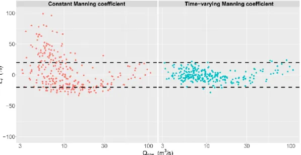
When aquatic vegetation is present, discharge predictions are improved when using a time-varying friction coefficient instead of a constant friction coefficient. Figure 2 shows the compar-ison of the relative errors for the model with constant friction coefficient (Eq. 1) with those for the new model with time-varying friction coefficient (Eq. 6). Relative errors can exceed 50% when the friction coefficient is constant whereas they mostly range between ± 20% when a time-varying friction coefficient is used. These results are promising since the uncertainty of the discharge measurements is equal to 15%.
Figure 2. Relative error Er as a function of the observed water discharge (Qobs) according to the chosen
rating curve model (with constant or time-varying Manning coefficient).
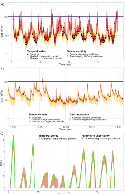
Figure 3a shows the discharge time series Q(t) with uncertainty, computed over the studied period using the continuous stage record at the station and our rating curve models. The 95% to-tal uncertainty interval is displayed on Figure 3a, including parametric (i.e. related to the param-eter estimation) and structural (i.e. related to the model) uncertainties. Solid lines correspond to the maxpost curves, which have been calculated with the parameters of the model maximising the posterior pdf (the Maximum A Posteriori estimators, MAP). The gaugings are best approxi-mated with the model with time-varying Manning coefficient (see the details for year 2008 in Fig. 3b for more clarity). The total discharge uncertainty is also much smaller.
Figure 3c presents the evolution of the proxy biomass with parametric uncertainty deduced from the model with time-varying Manning coefficient. Proxy biomass G(t) is strongly varying from year to year in both amplitude and shape. This reflects strong flow resistance variations hence the need to take into account bed roughness changes due to plant development when computing discharge for such hydrometric station.
4.2 Relative hydraulic importance of plant bending and development
In our new rating curve model, we assumed that two main effects drive the variations of the fric-tion coefficient related to the vegetafric-tion: the growth and decay of the plant (i.e. biomass evolu-tion) and the capacity of the plant to bend (i.e. its flexibility). The relative importance of these two effects is investigated. Discharges calculated when the bending correction is activated (Qbending) or not (Qno-bending) are compared. To evaluate Qno-bending, we use the same rating curve model as for estimating Qbending, except χ is set to 0 for evaluating the time-varying friction coef-ficient. Indeed, in case there is no bending, plants are assumed rigid so their reconfiguration co-efficients χ equal 0. The Newton-Raphson algorithm is no longer required for computing Q no-bending since the discharge is no longer present in the friction equation nv(t). To compute Q no-bending, we decide to use the same MAP parameters as those estimated when plant bending was taken into account, except for χ = 0. No new simulation is launched with the statistical tool BaM! in order to avoid compensating the absence of plant bending by other model parameter
during their estimation. That way, we investigate the importance (in terms of amplitude) of us-ing the bendus-ing correction in the global calibrated model (with bendus-ing).
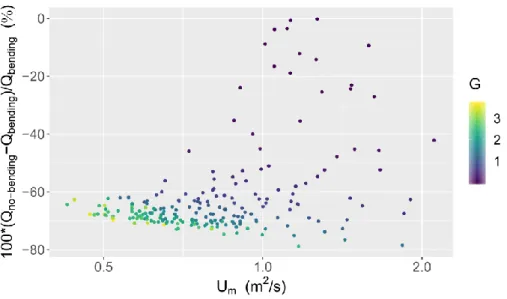
Figure 4 shows the relative discharge differences due to the plant bending function in the cal-ibrated model. Only observational data for which vegetation was present (i.e. when G(t) ≠ 0) are kept on Figure 4. The difference in discharge can reach up to 80%, which reflects the im-portance of the part related to the bending in the discharge computation with the new rating curve model. The variation in discharge seems correlated to the quantity of plant biomass and to
the gauged mean velocity. It is stronger if vegetation biomass is important and if gauged mean velocity is high. In addition, the variation is negative. As rigid plants grow, their frontal areas impacted by the flow become more important. They cannot bend or align in the flow direction to reduce them. The flow is thus obstructed and the discharge reduces. When Um<Uχ, the rela-tive difference should in theory go to zero. Unfortunately, no gauging was made in those condi-tions, so this statement cannot be verified.
Figure 3. a) Computed water discharge time series Q(t), b) details for year 12 (corresponding to year 2008) and c) evolution of the proxy biomass G(t) over the 11-year of data with uncertainty. Blue lines mark the transition to another hydraulic control for higher flows: computed discharges are not valid above these lines.
Figure 4. Relative discharge differences due to the plant bending function in the calibrated model with aquatic vegetation effect as a function of the gauged mean velocity and the proxy biomass at the station.
5 CONCLUSIONS
A rating curve model accounting for the presence of aquatic vegetation based on a time-varying friction coefficient was developed. It is restricted to hydraulic controls that can be described by the Manning-Strickler equation for wide rectangular channels and to submerged (with low rela-tive submergence), flexible or rigid macrophytes. The time-varying coefficient is estimated us-ing a friction equation accountus-ing for vegetation biomass evolution and for plant flexibility. The friction equation needs to be selected according to the type of plants growing at the station. The information needed to compute discharge is easily measurable or estimable (i.e. stage record, expertise on hydraulic controls and simple information about plants such as comments from visual observations), which makes the model interesting for operational purposes.
The performance of the model was highlighted using tests performed on a French hydromet-ric station affected by aquatic plants. The prediction of discharge was improved when rating curve models with varying friction coefficient are used, as opposed to constant friction coeffi-cient. Relative errors between computed and observed discharges ranged within ±20% with the new model. One interest of this new model is that the potential resistance of the plant related to its development can be modelled, which informs about the general trend of the plant evolution.
In this study, we emphasized the importance of the part related to the bending correction in the discharge calculation. Indeed, in certain conditions, not only the vegetation development but also the plant bending controlled the flow resistance related to plants. Results showed that the bending correction substantially modifies the estimated discharge (sometimes up to 80% com-pared to setting the bending correction to zero). The bending effect is particularly large when the mean velocity is high and when the plant biomass is significant.
REFERENCES
Aberle, J. & Järvelä, J. 2013. Flow resistance of emergent rigid and flexible floodplain vegetation.
Jour-nal of Hydraulic Research 51: 33-45.
Coon, W. 1998. Estimation of roughness coefficients for natural stream channels with vegetated banks.
U.S. Geological Survey Water Supply 244: 145.
Cowan, W.L. 1956. Estimating hydraulic roughness coefficients. Agricultural Engineering 37: 473-475. Green, J.C. 2005. Comparison of blockage factors in modelling the resistance of channels containing
submerged macrophytes. Rivers Research and Applications 21: 671-686.
Järvelä, J. 2004. Determination of flow resistance caused by non-submerged woody vegetation.
Lazár, A.N., Wade, A.J. & Moss, B. 2016. Modelling Primary Producer Interaction and Composition: an Example of a UK Lowland River. Environmental Modeling & Assessment 21: 125-148.
Le Coz, J., Renard, B., Bonnifait, L., Branger, F. & Le Boursicaud, R. 2014. Combining hydraulic knowledge and uncertain gaugings in the estimation of hydrometric rating curves: A Bayesian ap-proach. Journal of Hydrology 509: 573-587.
Limerinos, J.T. 1970. Determination of the Manning coefficient from measured bed roughness in natural channels. U.S. Geological Survey Water Supply Paper 1898-B.
Mansanarez, V., Renard, B., Le Coz, J., Lang, M. & Darienzo, M. 2019. Shift Happens! Adjusting Stage-Discharge Rating Curves to Morphological Changes at Known Times. Water Resources Research 55: 2876-2899.
Meyer-Peter, E., Müller, R. 1948. Formulas for bedload transport, Proc. of the 2nd IAHR Congress,
Stock-holm, Sweden: 39-64.
Morin, J., Leclerc, M. Secretan, Y. & Boudreau, P. 2000. Integrated two-dimensional macrophytes-hydrodynamic modeling. Journal of Hydraulic Research 38: 163-172.
Pasche, E., & Rouvé, G. 1985. Overbank flow with vegetatively roughened flood plains. Journal of
Hy-draulic Engineering 111: 1262-1278.
Perret, E., Le Coz, J. & Renard, B. in prep for 2020. A rating curve model accounting for stage-discharge cycles due to seasonal aquatic vegetation.
Petrik, S. & Bosmajian, G. 1975. Analysis of Flow through Vegetation. Journal of Hydraulic Division 101: 871-884.
Yin, X., Goudriaan, J., Lantinga, E.A., Vos, J. & Spiertz, H.J. 2003. A flexible sigmoid function of de-terminate growth. Annals of Botany 91: 361-371.