BINARY BLACK HOLES IN DENSE STAR CLUSTERS:
EXPLORING THE THEORETICAL UNCERTAINTIES
The MIT Faculty has made this article openly available.
Please share
how this access benefits you. Your story matters.
Citation
Chatterjee, Sourav, Carl L. Rodriguez, and Frederic A. Rasio.
“BINARY BLACK HOLES IN DENSE STAR CLUSTERS: EXPLORING
THE THEORETICAL UNCERTAINTIES.” The Astrophysical Journal
834, no. 1 (January 3, 2017): 68. © 2017 The American Astronomical
Society
As Published
http://dx.doi.org/10.3847/1538-4357/834/1/68
Publisher
IOP Publishing
Version
Final published version
Citable link
http://hdl.handle.net/1721.1/109564
Terms of Use
Article is made available in accordance with the publisher's
policy and may be subject to US copyright law. Please refer to the
publisher's site for terms of use.
BINARY BLACK HOLES IN DENSE STAR CLUSTERS: EXPLORING THE THEORETICAL UNCERTAINTIES
Sourav Chatterjee1, Carl L. Rodriguez1,2, and Frederic A. Rasio1
1
Center for Interdisciplinary Exploration & Research in Astrophysics(CIERA), Physics & Astronomy, Northwestern University, Evanston, IL 60202, USA;sourav.chatterjee@northwestern.edu
2
MIT-Kavli Institute for Astrophysics and Space Research 77 Massachusetts Avenue, 37-664H, Cambridge, MA 02139, USA Received 2016 March 2; revised 2016 October 10; accepted 2016 October 25; published 2017 January 3
ABSTRACT
Recent N-body simulations predict that large numbers of stellar black holes (BHs) could at present remain bound to globular clusters (GCs), and merging BH–BH binaries are produced dynamically in significant numbers. We systematically vary“standard” assumptions made by numerical simulations related to, e.g., BH formation, stellar winds, binary properties of high-mass stars, and IMF within existing uncertainties, and study the effects on the evolution of the structural properties of GCs, and the BHs in GCs. Wefind that variations in initial assumptions can set otherwise identical initial clusters on completely different evolutionary paths, significantly affecting their present observable properties, or even affecting the cluster’s very survival to the present. However, these changes usually do not affect the numbers or properties of local BH–BH mergers. The only exception is that variations in the assumed winds and IMF can change the masses and numbers of local BH–BH mergers, respectively. All other variations(e.g., in initial binary properties and binary fraction) leave the masses and numbers of locally merging BH–BH binaries largely unchanged. This is in contrast to binary population synthesis models for the field, where results are very sensitive to many uncertain parameters in the initial binary properties and binary stellar-evolution physics. Weak winds are required for producing GW150914-like mergers from GCs at low redshifts. LVT151012 can be produced in GCs modeled both with strong and weak winds. GW151226 is lower-mass than typical mergers from GCs modeled with weak winds, but is similar to mergers from GCs modeled with strong winds.
Key words: black hole physics – globular clusters: general – methods: numerical – methods: statistical – stars: black holes – stars: kinematics and dynamics
1. INTRODUCTION
Our understanding of how black holes(BHs) evolve inside star clusters has a long and varied history. Following the classic work by Spitzer (1969), it was suggested that old (∼12 Gyr)
globular clusters (GCs) cannot retain a significant BH population up to the present day. It was argued that, due to the much higher mass of BHs compared to typical stars, BHs will quickly (102Myr) mass segregate to form an isolated subcluster that is dynamically decoupled from the GC. Due to the small size, high density, and small number of objects in the subclusters, relaxation and strong encounters were expected to eject the majority of BHs on a timescale of ∼1 Gyr. Thus, at most a few BHs would remain in the old GCs observed in the Milky Way (MW, e.g., Kulkarni et al. 1993; Sigurdsson & Hernquist 1993; Portegies Zwart & McMillan2000; Kalogera et al. 2004). Furthermore, it was argued that if significant
numbers of BHs are present in today’s GCs, a subset of them might be in accreting binary systems, and detectable as X-ray sources. However, observations of luminous X-ray sources in the MW GCs prior to 2012 had suggested that all of these sources are accreting neutron stars and not BHs, consistent with the theoretical expectation at the time(e.g., van Zyl et al.2004; Lewin & van der Klis 2006; Altamirano et al. 2010, 2012; Bozzo et al.2011).
This classical picture started to change with recent discoveries of BH candidates in extragalactic GCs, character-ized by their super-Eddington luminosities and high variability on short timescales(Maccarone et al.2007; Irwin et al.2010).
More recently, with the completion of the upgraded Very Large Array (VLA), surveys combining radio and X-ray data for the MW GCs detected quiescent BHs by comparing their radio and X-ray luminosities (e.g., Strader et al. 2012; Chomiuk
et al.2013). Interestingly, the MW GCs containing the detected
BH candidates show large ranges in structural properties, indicating that the retention of BHs may be quite common. Several recent or ongoing surveys promise much richer observational constraints on this question (e.g., Strader et al.2013; Miller-Jones et al.2014a,2014b; Strader2014).
To be detectable either via electromagnetic signatures or via gravitational waves(GW) from BH–BH mergers, the BHs must be in binary systems with very specific ranges of properties. Although dynamical interaction can enhance the production of binaries containing a BH (BBHs) (e.g., Kundu et al. 2002; Pooley et al.2003), modern simulations find that the fraction of
BHs in binaries is typically low (e.g., Leigh et al. 2014; Morscher et al.2015). Hence, it has been argued that detection
of just a few BH candidates in GCs indicates the existence of a much larger population of BHs that are not detectable (e.g., Strader et al.2012; Umbreit2012; Morscher et al.2013,2015).
Indeed, recent numerical studies have found that BH ejection is not nearly as efficient as was previously thought. In these studies, it has been shown that the BH subcluster does not stay decoupled from the rest of the cluster for prolonged periods. The same interactions that eject BHs from the subcluster also cause it to expand and re-couple with the rest of the cluster, dramatically increasing the timescale for BH evaporation(e.g., Breen & Heggie2013; Morscher et al.2015; Wang et al.2016).
These simulations suggest that tens to thousands of BHs may remain in today’s GCs (e.g., Mackey et al. 2008; Moody & Sigurdsson2009; Aarseth2012; Morscher et al.2013,2015).
Most recently, Morscher et al. (2015) showed that the
presence of a significant number of BHs can dramatically alter the overall dynamical evolution of GCs. Through repeated cycles of core collapse and core re-expansion, BH dynamics
acts as a significant and persistent source of energy. On the other hand, the clustered environment and high frequency of strong scattering interactions, especially involving binaries, can change the numbers and properties of BBHs that form inside clusters (e.g., Rodriguez et al. 2015, 2016a; Antonini et al.2016). Both of these aspects intricately depend on several
physical processes, many of which lack strong observational constraints. For example, the distribution of the natal kicks the BHs receive can control how many of them will be directly ejected from the GCs immediately upon formation. Natal kicks also control the fraction of BHs that may retain their binary companions after SNe. The high end of the stellar initial mass function(IMF) determines how many BHs a cluster can form. The binary fraction and binary orbital properties can alter the binary stellar evolution of a BBH(or their progenitors), as well as the rate at which they take part in dynamical encounters. In addition, the ratio between the BH mass and the average stellar mass, also directly set by the IMF, determines the timescale for BHs to sink to the center. Answers to a wide variety of questions—such as how many BHs and BBHs a GC can retain at present, how many BBHs it can form over its whole lifetime, at what rate BHs and BBHs get ejected from the clusters, and how the BHs affect the overall evolution of the clusters—can potentially depend on these initial assumptions. Hence, we must understand the sensitivity of our models to initial conditions and assumptions that are poorly constrained by existing observations.
In this study, we vary the initial assumptions affecting high-mass stars and BHs that are usually considered “standard” in theoretical studies of clusters, within their observational uncertainties. In particular, we vary the stellar IMF, the birth-kick distribution for the BHs, and the primordial binary fraction and the binary properties for massive stars. We also vary the assumed prescription for mass loss via stellar winds. Further-more, we vary the galacto-centric distance (rG) and
metalli-cities. Starting from otherwise identical initial star clusters, we study how varying these assumptions affects BH populations, and the overall evolution andfinal observable properties of the host clusters. We also study how these initial assumptions affect the number and properties of merging BH–BH binaries. We put these findings in the context of the recent landmark detections of GWs from BH–BH mergers by Advanced LIGO (Abbott et al.2016a,2016b,2016c,2016d,2016e).
In Section 2we describe our numerical models and we list the initial assumptions that we vary. In Section 3 we define how we evaluate observable cluster properties from our models. In Section 4 we show how the various assumptions affect the overall evolution and final observable properties of star clusters. Section 5focuses on how these assumptions and resulting differences in the cluster evolution as a whole alter the binary properties of BHs. In Section6we focus on the numbers and properties of BH–BH mergers and put those results in the context of the recent discoveries of GWs (Abbott et al.
2016b,2016c,2016d). We summarize our results and conclude
in Section7.
2. NUMERICAL MODELS
We use our Hénon-type(Hénon1971) cluster Monte Carlo
(CMC) code, developed and rigorously tested in our group over the past 15 years(Joshi et al.2000,2001; Fregeau et al.2003; Chatterjee et al. 2010, 2013a, 2013b; Umbreit et al. 2012; Pattabiraman et al.2013). For a detailed description of the most
recent updates and parallelization, see Pattabiraman et al. (2013) and Morscher et al. (2015). The Monte Carlo approach
is more approximate than a direct N-body integration (e.g., Aarseth2010), but requires only a fraction of the computational
time. This rapidity allows us to fully explore the parameter space of dense star clusters. Results from CMC have been extensively compared to recent state-of-the-art N-body simula-tions, and were found to produce excellent agreement in all quantities of interest in this study(Rodriguez et al.2016c).
2.1. Standard Assumptions
In order to understand the influence of each initial assumption on the production and subsequent evolution of BHs in a cluster, we anchor our numerical models using the same assumptions as used in Morscher et al.(2015). We call
this our“standard” model and denote it as S (Tables1,2). Our
standard model initially has N=8×10⁵ stars. The position and velocities of the stars are set according to a King profile with W0=5 (King 1962, 1965, 1966). We adopt the
commonly used IMF presented in Kroupa (2001), and use
the central value for each slope in the different mass ranges between 0.1 and 100M to assign masses to these stars. In
modelS we assume an initial binary fraction fb=0.05. This is realized by randomly selecting the appropriate number (Nb= N × fb) of stars, independent of their masses or positions
in the cluster, and assigning binary companions to them. The mass of the secondary (ms) is drawn from a uniform
distribution with a lower limit taken from the assumed IMF, mmin=0.1M, and an upper limit equal to the mass of the
primary (mp). The orbital period (P) is drawn from a
distributionflat inlogP between 5 times the sum of the radii for the binary companions, and the local hard–soft boundary given by vorb=vσ, where, vorbis the orbital velocity and vσis
the local velocity dispersion. Note that, although all initial binaries are locally hard, dynamical evolution can make them soft at a later time, either by increasing the local velocity dispersion of other stars(typically in the core) or by moving the binary from its initial location to where the velocity dispersion is higher (due to mass segregation). Such soft binaries are maintained in all our simulations until strong scattering encounters disrupt them. The initial orbital eccentricities for the binaries are drawn from a thermal distribution.
Single and binary stellar evolution is performed with SSE and BSE (Hurley et al. 2000, 2002). We have modified the
prescription for stellar remnant formation in SSE and BSE by using the results of Fryer & Kalogera(2001) and Belczynski
et al. (2002). All core-collapsed neutron stars get birth kicks
drawn from a Maxwellian distribution with σ= sNS=
265 km s−1. We assume momentum ( p∣ ∣) conserving kicks for BHs following the prescription of Belczynski et al. (2002).
BHs formed via the direct collapse scenario do not get any natal kicks, since there is no associated explosion or mass loss. BHs formed with significant fallback get natal kicks calculated by initially sampling from the same kick distribution as the neutron stars, but reduced in magnitude according to the fractional mass of the fallback (xfb) material (see Morscher
et al. 2015, for a more detailed description of our standard modelS).
Below we describe how we vary the above-mentioned initial assumptions. In each case we describe only the assumptions we change relative to the baseline modelS, with all other initial conditions held constant.
2.2. Initial Binary Fraction and Binary Properties of Massive Stars
One source of uncertainty in setting up the initial conditions is whether the binary fraction depends on the stellar mass. We create two models, F0 and F1, varying the fraction of high-mass stars (>15M) that are initially in binaries ( fb,high). In
models F0 and F1, we adopt limiting initial values of fb,high=0 and 1, respectively (Tables 1, 2). We assign the
binaries in these two models such that the overall binary fraction fbis keptfixed at 0.05. In model F0, Nb=0.05×N
stars are randomly chosen from all stars with mass15Mand
are assigned as binaries. In model F1, we first assign all stars with mass >15M as binaries. We randomly choose the
appropriate residual number of low-mass stars (15M) and
assign them as binaries to make fb=0.05. In F0 and F1, the
distributions for the mass ratios (q) and the orbital properties are identical to model S.
In addition to the binary fraction in high-mass stars, the binary orbital properties can potentially affect both the formation and interaction rate of BHs in a cluster. The observed distributions of initial separations and q for binaries may have significant uncertainties and selection biases. To understand the effects of these initial assumptions, we create a set of models where we vary the initial binary properties of the high-mass(>15M) stars. In these models, we assume that the
initial fb,high=0.7, following the observational constraint provided in Sana et al. (2012). In addition, we choose an
initial period distribution described bydn dlogPµP-0.55for
the high-mass stars(Sana et al.2012). The number of binaries
for low-mass stars is again adjusted so that the overall fb is
≈0.05, similar to model S. We denote these models with “F0.7.” Within this variant, we also consider two different q distributions for the high-mass binaries. In one, we use a uniform distribution of q between q=mmin/mpand 1. These
models are denoted with the string “Ms0.1”. Another set of models uses the same uniform distribution in q, but within a
much smaller range, 0.6 and 1. We denote this set of models with the string“q0.6” (Tables1,2).
2.3. Natal Kick Distribution for BHs
It has been widely accepted that the neutron stars get large natal kicks when they form via core-collapse SNe(e.g., Cordes et al. 1993; Lyne & Lorimer 1994; Wang et al. 2006; Zuo2015). However, the magnitudes of natal kicks imparted to
BHs is still a matter of debate. Observational constraints come from modeling the kicks required to explain the positions and velocities of known BH X-ray binaries (XRB) in the MW galactic potential. Detailed analysis of individual BH XRBs results in widely varying constraints on their natal kick magnitudes (e.g., Brandt et al. 1995; Nelemans et al. 1999; Gualandris et al. 2005; Willems et al. 2005; Dhawan et al. 2007; Fragos et al. 2009; Wong et al. 2012, 2014).
Instead of modeling individual systems, Repetto et al. (2012)
and Repetto & Nelemans (2015) performed population
synthesis using different assumptions of natal kick distributions and compared their results with the positions of the observed BHs in the MW. They found that BHs may get large kicks, perhaps even as large as the neutron stars formed via core-collapse SNe. In addition, they did notfind evidence of a mass-dependent kick distribution, which would be expected for the widely used p∣ ∣-conserving kick prescription. Recent theoretical study of core-collapse SNe by Pejcha & Thompson(2015) also
suggests that the birth kicks may not be directly correlated with the BH mass. In short, the distribution of formation kicks for BHs is largely uncertain, even at the qualitative level.
In addition to the one used inS, we create models with three different natal kick distributions for the BHs. These models assume that the kick magnitudes are independent of the BH masses and xfb, and are drawn from a Maxwellian given by
σ=sBH. We adopt three variations that are obtained by using
sBH=sNS=265 km s−1(denoted by the string “K1”),
sBH=0.1 sNS(denoted by the string “K2”), and sBH=0.01
sNS(denoted by the string “K3”) in Tables1,2. Table 1
Naming Convention for Models String Meaning for initial property variations
S Our baseline model; we use“standard” assumptions for BH kicks, galacto-centric distance, IMF, fb, and Z (Section2.1).
Rx Galacto-centric distance is varied; rG=x kpc (Section2.6).
Z Metallicity is the same as in the baseline model, Z=0.001, independent of the galacto-centric distance of the cluster (Section2.6). In contrast, in other cases, we assume Z is anti-correlated with rGand assign metallicities consistent with the observed MW GCs at a given galacto-centric distance
(Djorgovski & Meylan1994).
fb0.1 Overall initial binary fraction is changed from ourfiducial value, fb=0.05, to fb=0.1 without changing the distributions of initial binary orbital
properties.
rv1 Initial rv=1 pc in contrast to our fiducial value of rv=2 pc.
Iw Wider range(0.08–150M) in the IMF is used relative to our fiducial range (0.1–100M).
Fx Binary fraction for high-mass(>15M) stars fb,high=x while keeping the overall binary fraction fb=0.05, the same as in the baseline model.
Ms0.1 Minimum secondary mass for initial binaries is 0.1M . In addition, the initial period distribution is taken from Sana et al. (2012).
q0.6 Minimum secondary mass for initial binaries is determined such that the mass ratio q=ms/mp 0.6. In addition, the initial period distribution is taken
from Sana et al.(2012).
Ki BH natal kicks are independent of fallback fraction and remnant mass. Indexi=1, 2, 3 denote sBH/sNS=1, 0.1, and 0.01, respectively.
Is Steep power-law exponent is used(α1= 3) for the IMF for stars more massive than 1M .
If Flat power-law exponent is used(α1= 1.6) for the IMF for stars more massive than 1M .
W Weak winds(Vink et al.2001) are assumed.
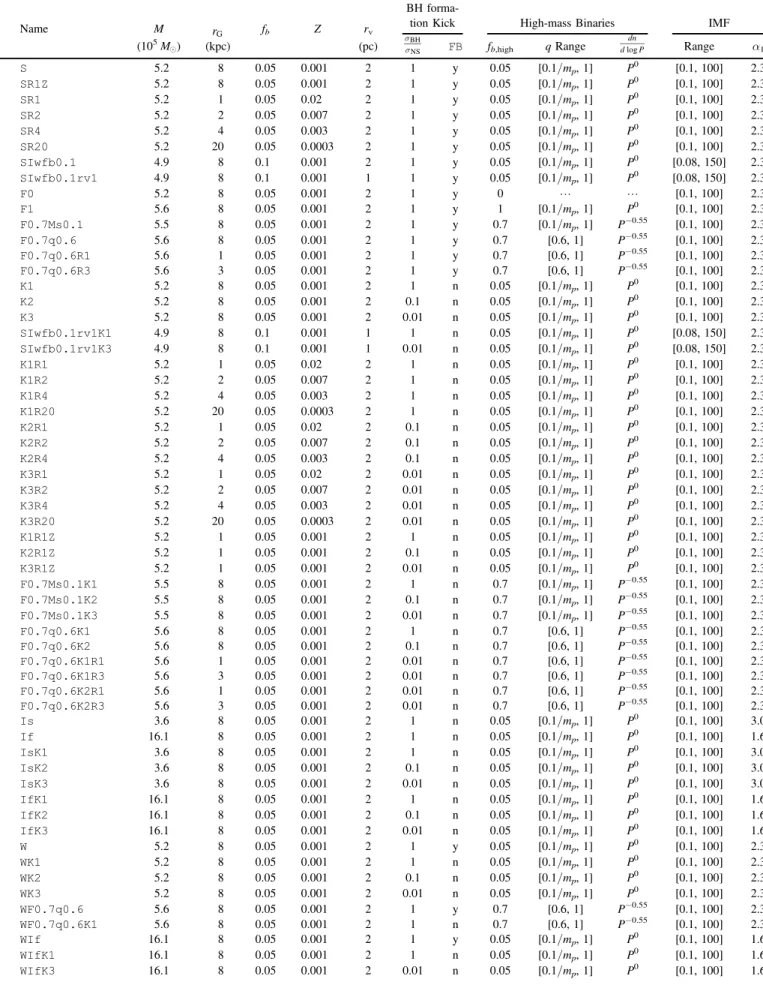
Note. We give informative names to our models. The names are combinations of several strings where each string refers to particular initial assumptions. To aid the readers understand the initial assumptions for particular models directly from the model’s name we list specific strings in the names of our models and their corresponding meaning for the initial assumptions.
Table 2 Initial Model Parameters
No. Name M rG fb Z rv
BH
forma-tion Kick High-mass Binaries IMF
(105 M ) (kpc) (pc) ss BH NS FB fb,high q Range dn dlogP Range α1 1 S 5.2 8 0.05 0.001 2 1 y 0.05 [0.1/mp, 1] P0 [0.1, 100] 2.3 2 SR1Z 5.2 8 0.05 0.001 2 1 y 0.05 [0.1/mp, 1] P0 [0.1, 100] 2.3 3 SR1 5.2 1 0.05 0.02 2 1 y 0.05 [0.1/mp, 1] P 0 [0.1, 100] 2.3 4 SR2 5.2 2 0.05 0.007 2 1 y 0.05 [0.1/mp, 1] P0 [0.1, 100] 2.3 5 SR4 5.2 4 0.05 0.003 2 1 y 0.05 [0.1/mp, 1] P0 [0.1, 100] 2.3 6 SR20 5.2 20 0.05 0.0003 2 1 y 0.05 [0.1/mp, 1] P 0 [0.1, 100] 2.3 7 SIwfb0.1 4.9 8 0.1 0.001 2 1 y 0.05 [0.1/mp, 1] P0 [0.08, 150] 2.3 8 SIwfb0.1rv1 4.9 8 0.1 0.001 1 1 y 0.05 [0.1/mp, 1] P0 [0.08, 150] 2.3 9 F0 5.2 8 0.05 0.001 2 1 y 0 L L [0.1, 100] 2.3 10 F1 5.6 8 0.05 0.001 2 1 y 1 [0.1/mp, 1] P0 [0.1, 100] 2.3 11 F0.7Ms0.1 5.5 8 0.05 0.001 2 1 y 0.7 [0.1/mp, 1] P−0.55 [0.1, 100] 2.3 12 F0.7q0.6 5.6 8 0.05 0.001 2 1 y 0.7 [0.6, 1] P−0.55 [0.1, 100] 2.3 13 F0.7q0.6R1 5.6 1 0.05 0.001 2 1 y 0.7 [0.6, 1] P−0.55 [0.1, 100] 2.3 14 F0.7q0.6R3 5.6 3 0.05 0.001 2 1 y 0.7 [0.6, 1] P−0.55 [0.1, 100] 2.3 15 K1 5.2 8 0.05 0.001 2 1 n 0.05 [0.1/mp, 1] P0 [0.1, 100] 2.3 16 K2 5.2 8 0.05 0.001 2 0.1 n 0.05 [0.1/mp, 1] P 0 [0.1, 100] 2.3 17 K3 5.2 8 0.05 0.001 2 0.01 n 0.05 [0.1/mp, 1] P0 [0.1, 100] 2.3 18 SIwfb0.1rv1K1 4.9 8 0.1 0.001 1 1 n 0.05 [0.1/mp, 1] P0 [0.08, 150] 2.3 19 SIwfb0.1rv1K3 4.9 8 0.1 0.001 1 0.01 n 0.05 [0.1/mp, 1] P 0 [0.08, 150] 2.3 20 K1R1 5.2 1 0.05 0.02 2 1 n 0.05 [0.1/mp, 1] P0 [0.1, 100] 2.3 21 K1R2 5.2 2 0.05 0.007 2 1 n 0.05 [0.1/mp, 1] P0 [0.1, 100] 2.3 22 K1R4 5.2 4 0.05 0.003 2 1 n 0.05 [0.1/mp, 1] P 0 [0.1, 100] 2.3 23 K1R20 5.2 20 0.05 0.0003 2 1 n 0.05 [0.1/mp, 1] P 0 [0.1, 100] 2.3 24 K2R1 5.2 1 0.05 0.02 2 0.1 n 0.05 [0.1/mp, 1] P0 [0.1, 100] 2.3 25 K2R2 5.2 2 0.05 0.007 2 0.1 n 0.05 [0.1/mp, 1] P0 [0.1, 100] 2.3 26 K2R4 5.2 4 0.05 0.003 2 0.1 n 0.05 [0.1/mp, 1] P 0 [0.1, 100] 2.3 27 K3R1 5.2 1 0.05 0.02 2 0.01 n 0.05 [0.1/mp, 1] P0 [0.1, 100] 2.3 28 K3R2 5.2 2 0.05 0.007 2 0.01 n 0.05 [0.1/mp, 1] P0 [0.1, 100] 2.3 29 K3R4 5.2 4 0.05 0.003 2 0.01 n 0.05 [0.1/mp, 1] P 0 [0.1, 100] 2.3 30 K3R20 5.2 20 0.05 0.0003 2 0.01 n 0.05 [0.1/mp, 1] P0 [0.1, 100] 2.3 31 K1R1Z 5.2 1 0.05 0.001 2 1 n 0.05 [0.1/mp, 1] P0 [0.1, 100] 2.3 32 K2R1Z 5.2 1 0.05 0.001 2 0.1 n 0.05 [0.1/mp, 1] P 0 [0.1, 100] 2.3 33 K3R1Z 5.2 1 0.05 0.001 2 0.01 n 0.05 [0.1/mp, 1] P0 [0.1, 100] 2.3 34 F0.7Ms0.1K1 5.5 8 0.05 0.001 2 1 n 0.7 [0.1/mp, 1] P−0.55 [0.1, 100] 2.3 35 F0.7Ms0.1K2 5.5 8 0.05 0.001 2 0.1 n 0.7 [0.1/mp, 1] P−0.55 [0.1, 100] 2.3 36 F0.7Ms0.1K3 5.5 8 0.05 0.001 2 0.01 n 0.7 [0.1/mp, 1] P−0.55 [0.1, 100] 2.3 37 F0.7q0.6K1 5.6 8 0.05 0.001 2 1 n 0.7 [0.6, 1] P−0.55 [0.1, 100] 2.3 38 F0.7q0.6K2 5.6 8 0.05 0.001 2 0.1 n 0.7 [0.6, 1] P−0.55 [0.1, 100] 2.3 39 F0.7q0.6K1R1 5.6 1 0.05 0.001 2 0.01 n 0.7 [0.6, 1] P−0.55 [0.1, 100] 2.3 40 F0.7q0.6K1R3 5.6 3 0.05 0.001 2 0.01 n 0.7 [0.6, 1] P−0.55 [0.1, 100] 2.3 41 F0.7q0.6K2R1 5.6 1 0.05 0.001 2 0.01 n 0.7 [0.6, 1] P−0.55 [0.1, 100] 2.3 42 F0.7q0.6K2R3 5.6 3 0.05 0.001 2 0.01 n 0.7 [0.6, 1] P−0.55 [0.1, 100] 2.3 43 Is 3.6 8 0.05 0.001 2 1 n 0.05 [0.1/mp, 1] P 0 [0.1, 100] 3.0 44 If 16.1 8 0.05 0.001 2 1 n 0.05 [0.1/mp, 1] P 0 [0.1, 100] 1.6 45 IsK1 3.6 8 0.05 0.001 2 1 n 0.05 [0.1/mp, 1] P0 [0.1, 100] 3.0 46 IsK2 3.6 8 0.05 0.001 2 0.1 n 0.05 [0.1/mp, 1] P0 [0.1, 100] 3.0 47 IsK3 3.6 8 0.05 0.001 2 0.01 n 0.05 [0.1/mp, 1] P 0 [0.1, 100] 3.0 48 IfK1 16.1 8 0.05 0.001 2 1 n 0.05 [0.1/mp, 1] P0 [0.1, 100] 1.6 49 IfK2 16.1 8 0.05 0.001 2 0.1 n 0.05 [0.1/mp, 1] P0 [0.1, 100] 1.6 50 IfK3 16.1 8 0.05 0.001 2 0.01 n 0.05 [0.1/mp, 1] P 0 [0.1, 100] 1.6 51 W 5.2 8 0.05 0.001 2 1 y 0.05 [0.1/mp, 1] P0 [0.1, 100] 2.3 52 WK1 5.2 8 0.05 0.001 2 1 n 0.05 [0.1/mp, 1] P0 [0.1, 100] 2.3 53 WK2 5.2 8 0.05 0.001 2 0.1 n 0.05 [0.1/mp, 1] P 0 [0.1, 100] 2.3 54 WK3 5.2 8 0.05 0.001 2 0.01 n 0.05 [0.1/mp, 1] P0 [0.1, 100] 2.3 55 WF0.7q0.6 5.6 8 0.05 0.001 2 1 y 0.7 [0.6, 1] P−0.55 [0.1, 100] 2.3 56 WF0.7q0.6K1 5.6 8 0.05 0.001 2 1 n 0.7 [0.6, 1] P−0.55 [0.1, 100] 2.3 57 WIf 16.1 8 0.05 0.001 2 1 y 0.05 [0.1/mp, 1] P0 [0.1, 100] 1.6 58 WIfK1 16.1 8 0.05 0.001 2 1 n 0.05 [0.1/mp, 1] P0 [0.1, 100] 1.6 59 WIfK3 16.1 8 0.05 0.001 2 0.01 n 0.05 [0.1/mp, 1] P 0 [0.1, 100] 1.6
2.4. Initial Stellar Mass Function
A lot of observational effort is aimed towards finding the expected IMF for stars born in clusters (e.g., Kroupa & Boily2002, and the references therein). Of course, the number of BHs a cluster can form is directly dependent on the number of massive BH-progenitor stars it initially contains. This, in turn, is directly dependent on the stellar IMF, especially the power-law slope of the IMF near the high-end of stellar masses. As described earlier, our standard models use the central values for the IMF slopes from Kroupa(2001). However, we note that
the best-fit power-law exponents α in dn/dm∝m− α through-out all mass ranges have large uncertainties. For example, the power-law exponent α1, for stars more massive than 1M is
2.3 with 1σ error of 0.7 (Kroupa2001). We vary α1within the
quoted 1σ uncertainties, and create models with α1=1.6
(denoted using the string “If”) and α1=3 (denoted using the
string“Is”) in Tables 1,2.
2.5. Stellar Wind Prescription
The details of how stars lose mass to stellar winds is complicated and hard to model theoretically. Most stellar evolution prescriptions instead model the mass and metallicity-dependent stellar winds by calibrating the wind-driven mass loss to catalogs of observed stars(e.g., de Boer et al.1997; Van Eck et al. 1998; Hurley et al. 2000; Vink et al. 2001). The
assumed wind prescription dramatically affects the mass of the BH progenitor at the time of SN, which in turn determines the mass of the resultant BH. The wind prescription described in Hurley et al.(2000) is widely used as part of the SSE and BSE
software packages in many widely used cluster dynamics codes. The majority of our models use this stellar wind prescription. For simplicity, we call BSE’s implementation for winds the“strong wind” prescription.
Recent observations of high-mass stars suggest that the stellar winds may not be as strong as suggested by earlier studies (e.g., Vink et al. 2001; Vink 2008; Belczynski et al. 2010a,2010b; Dominik et al. 2012; Spera et al. 2015).
The details of this wind prescription, based on e.g., Vink et al. (2001), are documented in detail in Belczynski et al. (2010b),
and implemented in our code (Rodriguez et al. 2016a). For
simplicity, we call this implementation the “weak wind” prescription. All models adopting weak winds are denoted with the string“W” in Tables1,2.
2.6. Other Assumptions
In addition to the above variations to our standard modelS, we also vary the galacto-centric distance (rG), metallicity (Z),
the initial virial radius(rv), and the overall spread in the stellar
IMF for a handful of models.
For easier understanding of the variations of initial assumptions in specific models we name all models in such a way that specific strings in the name indicate specific variations. In Table 1 we summarize the specific strings in model names and what they mean. All model names are created using some combination of these strings indicating combina-tions of specific initial assumptions. The details of all models and initial assumptions are listed in Table1.
3. DERIVATION OF OBSERVED CLUSTER PROPERTIES The definitions for key structural properties in numerical models are often different from those defined by observers for real clusters(e.g., Chatterjee et al.2013b). To be consistent, we
“observe” our simulated models to extract structural properties with definitions similar to those used for real observations. We use the last snapshot from all our model clusters to extract the observable structural properties. All relevant final structural properties, measured both using theoretical definitions, and observers’ definitions are listed in Table3.
3.1. Estimation of “Observed” Structural Properties We create two-dimensional projections for each model assuming spherical symmetry. The half-light radius, rhl,obs, is
then estimated byfinding the projected radius containing half of the total light. We obtain the observed core radius, rc,obs, and
the observed central density, Sc,obs, byfitting an analytic King
model to the cumulative stellar luminosity at a given projected radius including stars within a projected distance of rhl,obsfrom
the center (King1962, their Equation(18)). This method was suggested previously by Morscher et al. (2015). Since, this
approach avoids binning of data, it is more robust against statistical fluctuations, especially at low projected distances, compared to the often-used method offitting the King profile directly to the surface brightness profile (SBP).
We estimate the observed central velocity dispersion vσ,c,obs
by taking the standard deviation of the magnitudes of the three-dimensional velocities of all luminous stars(excluding compact objects) within a projected distance of rc,obs. In the case of
binaries, we take into account the center of mass velocities.
3.2. Estimation of Dissolution Times
Depending on initial assumptions, some of our cluster models get tidally disrupted before the integration stopping time of 12 Gyr. The basic assumptions of our Monte Carlo approach are spherical symmetry, and a sufficiently large N to ensure that the relaxation timescale is significantly longer than
Table 2 (Continued)
No. Name M rG fb Z rv
BH
forma-tion Kick High-mass Binaries IMF
(105 M ) (kpc) (pc) ssBHNS FB fb,high q Range dn dlogP Range α1 60 Wrv1fb0.1 5.0 8 0.1 0.001 1 1 y 0.1 [0.1/mp, 1] P0 [0.08, 150] 2.3 61 Wrv1K1fb0.1 5.0 8 0.1 0.001 1 1 n 0.1 [0.1/mp, 1] P 0 [0.08, 150] 2.3 62 Wrv1K3fb0.1 5.0 8 0.1 0.001 1 0.01 n 0.1 [0.1/mp, 1] P0 [0.08, 150] 2.3
Note. Each model initially has N=8×10⁵stars. ColumnFB denotes whether or not natal kicks for BHs are dependent on fallback. α
1denotes the magnitude of the
Table 3
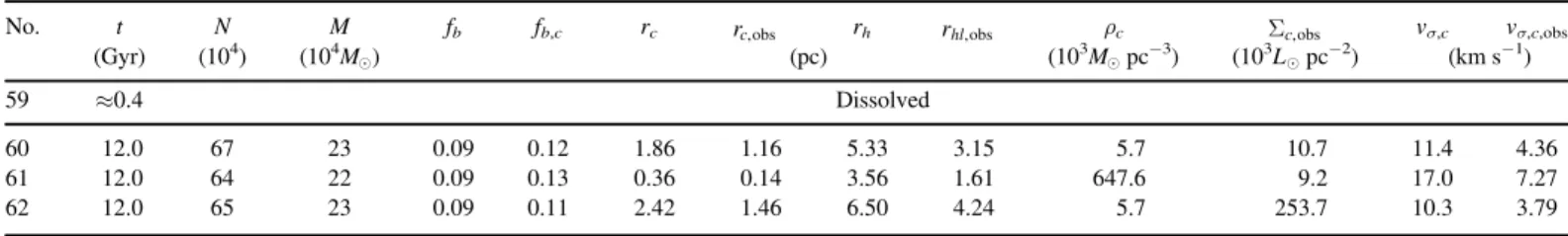
Final Structural Properties of Model Clusters
No. t N M fb fb,c rc rc,obs rh rhl,obs ρc Sc,obs vσ,c vσ,c,obs
(Gyr) (104) (104 M ) (pc) (103 M pc−3) (103 L pc−2) (km s−1) 1 12.0 71 26 0.05 0.05 2.90 3.06 7.89 5.55 17.8 1.9 9.8 3.40 2 ≈5 Dissolved 3 12.0 24 12 0.06 0.13 0.64 0.40 2.80 1.41 44.0 31.5 10.9 4.26 4 12.0 55 21 0.05 0.06 2.52 2.86 6.12 4.01 9.1 2.2 9.8 3.32 5 12.0 68 25 0.05 0.06 2.83 2.59 7.16 4.73 12.3 2.0 9.9 3.46 6 12.0 73 27 0.05 0.05 3.07 4.22 8.54 6.24 21.8 1.5 9.7 3.30 7 12.0 76 26 0.09 0.12 1.89 1.12 5.65 3.27 7.5 9.2 11.5 4.37 8 12.0 71 25 0.09 0.14 0.83 1.12 4.29 3.27 28.7 9.2 13.6 5.30 9 12.0 71 26 0.05 0.05 3.20 2.63 7.82 5.50 3.2 2.2 9.9 3.46 10 12.0 73 27 0.04 0.05 2.51 3.34 7.71 5.39 121.1 1.9 9.8 3.46 11 12.0 73 27 0.04 0.05 3.15 2.81 7.77 5.44 5.6 2.4 10.0 3.47 12 12.0 73 27 0.04 0.05 3.05 5.07 8.12 5.73 20.6 1.4 9.7 3.24 13 ≈4 Dissolved 14 12.0 63 24 0.04 0.05 3.05 2.24 7.54 5.25 14.0 2.4 9.2 3.23 15 12.0 77 28 0.04 0.11 0.36 0.22 4.98 2.47 275.1 126.6 14.2 6.08 16 12.0 76 27 0.05 0.07 2.00 1.42 5.71 3.48 8.3 7.6 11.7 4.38 17 12.0 70 26 0.05 0.05 3.09 3.73 8.20 5.90 9.1 1.3 9.7 3.30 18 12.0 69 23 0.08 0.13 0.32 0.22 4.56 2.17 371.1 121.3 14.9 6.41 19 12.0 69 24 0.09 0.12 1.41 1.12 5.00 2.90 68.7 122.9 12.1 4.64 20 12.0 30 14 0.05 0.14 0.20 0.17 3.05 1.30 678.2 126.0 12.0 4.92 21 12.0 66 25 0.04 0.12 0.37 0.05 4.54 2.02 226.6 2121.9 13.5 5.57 22 12.0 74 27 0.04 0.11 0.55 0.25 4.93 2.26 96.1 88.4 13.5 5.58 23 12.0 77 28 0.04 0.10 0.32 0.26 5.07 2.67 384.3 92.7 14.7 6.42 24 12.0 24 12 0.06 0.13 0.65 0.48 2.78 1.36 36.8 35.0 11.0 4.26 25 12.0 63 24 0.05 0.07 1.70 1.28 4.91 2.75 4.4 8.2 11.7 4.35 26 12.0 73 26 0.05 0.07 2.06 1.74 5.67 3.31 3.9 5.2 11.5 4.19 27 12.0 12 6 0.07 0.12 0.77 1.11 2.82 1.87 79.3 5.3 7.7 2.79 28 12.0 53 21 0.05 0.06 2.45 2.06 6.27 4.19 17.0 2.9 9.5 3.32 29 12.0 67 24 0.05 0.06 2.80 3.99 7.36 5.06 15.5 1.5 9.7 3.30 30 12.0 73 27 0.05 0.05 3.30 2.28 8.63 6.26 5.0 2.4 9.8 3.45 31 12.0 28 13 0.05 0.12 0.18 0.14 2.77 1.52 1124.2 205.1 13.7 5.78 32 12.0 20 10 0.06 0.09 1.02 1.44 2.89 1.92 13.9 8.1 9.7 3.39 33 ≈4 Dissolved 34 12.0 77 28 0.04 0.09 0.59 0.31 5.08 2.63 68.2 66.2 13.4 5.61 35 12.0 76 28 0.04 0.06 2.22 1.39 6.00 3.74 3.2 7.9 11.4 4.25 36 12.0 73 27 0.04 0.05 3.09 2.26 7.85 5.45 7.3 2.9 10.0 3.53 37 12.0 78 28 0.04 0.09 0.71 0.36 5.18 2.66 42.6 58.2 13.1 5.42 38 12.0 76 28 0.04 0.06 2.45 1.89 6.47 4.20 6.7 4.4 11.0 4.00 39 12.0 26 12 0.05 0.13 0.20 0.31 2.73 1.53 616.9 55.7 12.4 5.01 40 12.0 71 26 0.04 0.09 0.68 0.59 4.87 2.55 58.7 26.9 13.1 5.31 41 12.0 7 4 0.07 0.09 0.92 0.73 2.48 1.78 10.8 6.4 7.0 2.49 42 12.0 69 26 0.04 0.06 2.23 1.20 5.85 3.76 8.3 8.4 11.0 4.05 43 12.0 71 25 0.04 0.09 0.29 0.13 4.28 1.68 384.7 335.5 15.4 6.67 44 ≈2 Dissolved 45 12.0 74 25 0.04 0.07 0.21 0.18 4.63 2.06 966.6 175.1 13.5 5.85 46 12.0 72 25 0.04 0.08 0.20 0.14 4.46 1.97 1107.9 260.7 13.8 5.93 47 12.0 71 25 0.04 0.10 0.36 0.10 4.14 1.61 286.1 646.3 15.7 6.83 48 <0.1 Dissolved 49 ≈3 Dissolved 50 ≈2 Dissolved 51 12.0 69 25 0.05 0.05 3.58 4.72 8.57 6.17 3.7 1.1 9.3 3.10 52 11.0 77 28 0.04 0.10 0.56 0.26 4.73 2.31 89.7 112.1 14.5 6.06 53 12.0 74 27 0.05 0.06 2.50 1.57 6.28 4.07 2.6 5.8 11.0 4.05 54 12.0 63 24 0.05 0.05 3.96 7.76 10.55 7.95 10.4 0.5 8.2 2.58 55 12.0 69 26 0.04 0.05 3.64 2.20 8.38 5.90 2.4 2.4 9.4 3.31 56 12.0 77 28 0.04 0.09 0.76 0.56 5.09 2.61 34.4 35.1 13.3 5.49 57 ≈0.6 Dissolved 58 12.0 60 24 0.04 0.04 13.95 35.76 21.29 16.29 0.0 0.1 4.8 1.34
the dynamical timescale. Both assumptions break down for clusters that have begun to tidally disrupt, since the tidal boundary is not spherically symmetric, and a disrupting cluster can lose mass on a timescale = than the relaxation time. To that end, oncet tr( )>M t( ) M˙ for a cluster, where tr, and M
denote relaxation time and total cluster mass respectively, we consider the cluster to have dissolved. For clusters that dissolve before 12 Gyr, we list the approximate dissolution times and mark them as “Dissolved” in Table3.
4. OVERALL CLUSTER EVOLUTION
Figure1shows the evolution of the core radius(rc) and the
half-mass radius(rh) for our standard model S. As expected, rc
shows repeated downward spikes indicating collapse of the BH subcluster (e.g., Morscher et al. 2015). Dynamical ejections
and binary formation following each BH-driven core collapse produce energy, reversing the collapse and re-expanding the BH positions to mix with the rest of the cluster. Through repeated collapses, the rc increases on an average until the
integration is stopped at 12 Gyr, and attains rc=2.8±0.1 pc.
The error bar here denotes the 1σ fluctuations during the last 1 Myrof the cluster’s evolution. rhmonotonically increases as
well, attaining a final value of about 8 pc.
Of course, an astronomer observing this cluster would measure different values for the structural quantities. Since the core collapse at any time during the evolution involves only a small number of the most massive BHs in the cluster, the observable SBP is insensitive to these collapses. For example, Figure 2 shows the SBPs for the same model cluster at two different times during its evolution, one when the cluster is in a core-collapsed state and the other when the cluster is out of it. There is no difference between the SBPs, although the theoretical rc changes from about 0.4 to 2.8 pc between the
collapsed and non-collapsed states. Thus, the core collapses driven by BH dynamics in these clusters are not observable.
Figure 3 shows the SBP including stars with luminosity Lå20 Lefor model S at t=12 Gyr. At this time model S
has Sc,obs≈2.7×10³L pc -2, rhl,obs=5.5 pc, and
rc,obs=3 pc. Hence, to an observer S would appear as a
cluster with low central density and puffed-up core.
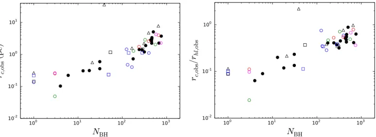
In general, if a large number of BHs remain bound to the host cluster, dynamics involving BHs(dynamical formation of new binaries, binary–single and binary–binary scattering, and dynamical ejections from the cluster core) acts as the dominant source of energy in the core. The cluster can start the relaxation-driven core-contraction phase only after this source of energy is sufficiently depleted. The larger the number of retained BHs (NBH) at a given time, the bigger the rc,obs and
rc,obs/rhl,obs for the host cluster (Figure 4). For example,
excluding the disrupted clusters, the correlation coefficient between NBH and rc,obs at t=12 Gyr is 0.82 and that between
rc,obs/rhl,obsis 0.78. Because of the large amount of energy
BH-driven dynamics can inject into the clusters, the central density, Sc,obs, also depends strongly on NBH; Sc,obs and NBH are
anti-correlated with a correlation coefficient of −0.3 (Figure5).
Table 3 (Continued)
No. t N M fb fb,c rc rc,obs rh rhl,obs ρc Sc,obs vσ,c vσ,c,obs
(Gyr) (104 ) (104 M ) (pc) (103M pc −3) (103L pc −2) (km s−1) 59 ≈0.4 Dissolved 60 12.0 67 23 0.09 0.12 1.86 1.16 5.33 3.15 5.7 10.7 11.4 4.36 61 12.0 64 22 0.09 0.13 0.36 0.14 3.56 1.61 647.6 9.2 17.0 7.27 62 12.0 65 23 0.09 0.11 2.42 1.46 6.50 4.24 5.7 253.7 10.3 3.79
Note. Serial numbers for models are the same as in Table2. Observed structural properties are denoted by the subscript“obs.” Definitions for observed properties are explained in Section3. The approximate dissolution times(Section3.2) are listed for dissolved clusters.
Figure 1. Evolution of the core radius (rc) and the half-mass radius (rh) for
model S. The solid (black) and dashed (blue) lines denote rc and rh,
respectively. The spikes in rcdue to BH-driven core collapse continue until the
end of the simulation at 12 Gyr. Both rcand rhexpand all the way to the end.
Figure 2. Comparison between the SBPs at two different times, one corresponding to a core-collapsed state, seen as the downward spikes in Figure 1 (at t = 9.27 Gyr; black), and the other corresponding to a non-collapsed state(at t = 9.29 Gyr; red) for model S. The theoretically defined core radius changes from rc≈0.4 during the collapsed state to about 3 pc out
Note that, due simply to the differences in the initial assumptions affecting the high-mass stars, clusters with very similar initial conditions attain widely varying final properties spanning ∼4 orders of magnitude in NBH, 2 orders of
magnitude in rc,obs, and 4 orders of magnitude in Sc,obs at
t=12 Gyr (Section 2; Tables 2and 3).
Wefind that the most dramatic differences in the overall final properties of a star cluster come from the differences in NBH.
The variations in initial assumptions can change the evolution of NBH in different ways, and as a result, change the overall
evolution of the cluster and its structural properties(e.g., rc,obs,
rhl,obs, and Sc,obs).
Wefind that the most important assumption that determines the evolution of NBH in a cluster is the natal kick distribution
for the BHs. Hence, we start by discussing the effects of initial assumptions related to BH-formation kicks.
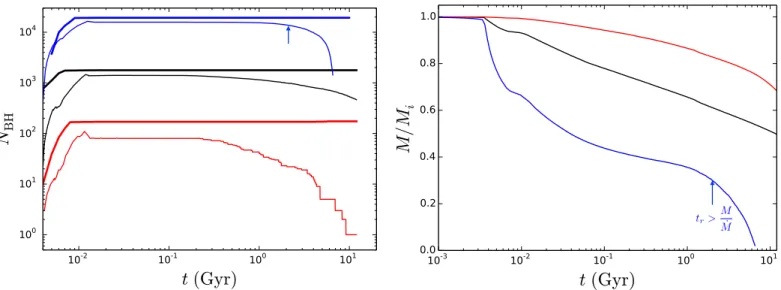
4.1. Effects of the Natal Kick Distribution for BHs The assumed natal kick distribution for BHs directly controls NBH at a given time, and through that it controls the evolution
of the cluster. For example, Figure 6 shows the evolution of NBH, rc, rh, rc/rh, and thefinal SBPs for four identical models,
all at a fixed rG=8 kpc. These models vary only in the
assumed distribution of natal kicks for the BHs. Wefind that if the BHs are given full NS kicks, i.e., sBH=sNS, most of the
BHs are ejected from the cluster within t≈20 Myr, immedi-ately after formation. Without the source of energy from BH dynamics at the center, the cluster starts contracting due to two-body relaxation after the initial expansion from mass loss via stellar evolution. At about 11 Gyr the cluster reaches the so-called binary-burning phase, when core-contraction is arrested due to extraction of binding energy from binary orbits via super-elastic scattering encounters (e.g., Heggie & Hut2003).
Based on the final SBP, this cluster would appear as a high-density core-collapsed cluster (Figure 6; see also Chatterjee et al.2013b). In contrast, clusters modeled with other natal kick
distributions, where the BHs essentially receive much lower kicks compared to the neutron stars formed via core-collapse SN, do retain large numbers of BHs all the way through 12 Gyr. Due to the energy produced from BH dynamics, each
of these clusters continues to expand until the end. K2 with sBH=0.1 sNS contains about 200 BHs at t=12 Gyr, a
sufficient number to keep the cluster in an expanded state. However, the rate of expansion is lower compared to modelsS andK3 where, at 12 Gyr, NBH are much higher, with values of
464 and 759, respectively. While near the end there are indications that the model cluster K2 would start contracting after it ejects some more BHs, models S and K3 are still expanding at t=12 Gyr, and appear as puffy, low-density clusters from their final SBPs. The same initial cluster can evolve to a final observational state with rc,obs and Sc,obs
varying by orders of magnitude, simply because of changes in the assumed natal kick distribution for its BHs(Table3).
The significant number of retained BHs can also expand the cluster closer to its tidal radius, making the cluster more prone to disruption from Galactic tides. For example, with otherwise the exact same properties, at rG=1 kpc, clusters with
relatively larger NBH expand more (e.g., SR1Z and K3R1Z),
and dissolve much earlier than 12 Gyr. On the other hand, with the same initial conditions, model clusters with relatively lower NBH are safe from tidal disruption even at rG=1 kpc (e.g.,
K1R1, K2R1; Table3).
In general, the larger the value of NBH, the lower thefinal
total mass of the cluster. This is because higher NBH expands
the cluster more, and a more expanded cluster loses more mass due to galactic tides. The exact amount of expansion, mass loss, and thefinal cluster mass also depends on the metallicity (Z) of the cluster, since the metallicity controls the wind-driven mass loss and the resulting mass of the BH population. Higher Z leads to the formation of lower-mass BHs, and as a result the overall expansion due to BH ejections is reduced. The adopted wind prescription yields a similar effect. While the strong wind prescription leads to a higher mass loss at early times compared to the weak wind prescription, the latter leads to the formation of more massive BHs in a cluster than the former. As a result, the same initial cluster under the weak wind assumption eventually undergoes more expansion when the energy production in the center is dominated by BH dynamics. This increased expansion leads to an increased rate of star loss in models with weak winds compared to those with strong winds, which is reflected in the final N in these clusters (Table 3).
4.2. Effects of the Assumed IMF
While for a given IMF the BH natal kick distribution is the dominant factor controlling BH retention and overall star cluster evolution, any change to the IMF, especially for the high-mass stars, can also bring about dramatic differences in how the cluster evolves. By directly controlling both the number of high-mass stars formed in a cluster (hence the number of BHs, stellar evolution driven mass loss), and the average stellar mass, variations in IMF can control the evolution of a cluster and even its survival (Chernoff & Weinberg1990; Banerjee & Kroupa 2011).
We have tested the effects of variation in the exponentα1of
the IMF for stars more massive than 1M within the quoted
uncertainty 2.3±0.7 in Kroupa (2001). Clusters evolve very
differently depending on the choice ofα1(Figure 7). We first
focus on our standard set of models(models S, Is, and If; Table2). While models with α1=2.3 and 3.0 evolve normally
and survive until t=12 Gyr, the model with α1=1.6
dissolves at around 2 Gyr(see Section3.2for how dissolution times are estimated). At first, mass is lost primarily via stellar
Figure 3. Final SBP at t=12 Gyr for model S. The dots denote the surface luminosity density. While calculating the SBP, we discard stars brighter than 20L to reduce noise from a small number of bright giant stars (e.g., Noyola &
Gebhardt 2006). The horizontal line denotes the central surface luminosity density(Sc,obs) based on the best-fit King model (Section3). The vertical lines denote the observed core radius rc,obs(obtained from the King fit) and observed
winds. Cluster modelIf loses slightly more mass compared to the other model clusters with steeperα1. Dramatic differences
appear during the stage when the clusters lose mass via compact object formation. As expected, the steeper the high-end of the IMF, the lower the mass loss from compact object formation. This episode of quick mass loss ends by the time all the BHs are formed and many of the BHs are ejected due to their birth kicks. Following this episode, mass loss slows down and is driven by dynamical ejections of BHs from the core and mass loss through the tidal boundary. At this stage, the number of retained BHs in a cluster becomes very important. A larger value of NBHleads to more dynamical ejections, which in turn
leads to faster cluster expansion and higher tidal mass loss rate. Eventually, if the cluster expands too much, it gets disrupted.
The details of this process depend both on the kick distribution for the BHs as well as the wind-driven mass loss (Figure 8). During the initial stages, clusters modeled with
weak winds lose less mass than those modeled with strong winds. However, lower wind-driven mass loss leads to the formation of more massive BHs. These higher-mass BHs segregate more rapidly in the cluster potential. In addition, higher-mass BHs inject more energy into the cluster via dynamics and ejections than their lower-mass counterparts. As a result, once the cluster is sufficiently old for BH dynamics to dominate energy production, the clusters modeled with weak winds expand faster and get disrupted earlier than those modeled with strong winds. The higher the number of retained BHs, the bigger the difference between the clusters modeled with strong and weak winds(Figure8). This trend is reversed
in the models IfK1 and WIfK1, both modeled with the highest natal kicks for the BHs we consider(Table2). Since in
these models almost all BHs are ejected during formation, the above-mentioned difference due to BH dynamics is not relevant. Instead, since in the high-kick case the weak wind model loses less mass than the strong wind model, IfK1 is disrupted earlier than WIfK1. To further illustrate this point, Figure9 shows the effects of α1on models with sBH=sNS.
Since most BHs are ejected during formation from all of these models(K1, WK1, IfK1, WIfK1) the evolution really depends only on the mass loss from compact object ejections during formation, i.e., the number of high-mass stars formed in the cluster.
4.3. Effects of Other Assumptions
The process and timescale for energy production from BH dynamics depend critically on the mass segregation timescale (tS) in a cluster (e.g., Breen & Heggie 2013; Morscher
et al.2013,2015). The mass segregation timescale of a massive
object depends on the relaxation timescale(tr), and the ratio of
its mass to the average stellar mass(〈m〉) in its neighborhood, µ á ñ
tS tr m
mi (e.g., Gürkan et al.
2004). Thus, NBHand as a result,
the overall cluster evolution, depend on assumptions such as: initial virial radius(rv), and the IMF, which can affect either tr
or á ñm
mi. Figure10shows the difference in the evolution of two
clusters(W and Wrv1fb0.1) with different initial rvand the Figure 4. Final number of BHs bound to the cluster, NBHvs. rc,obs(left) and rc,obs/rhl,obs(right) for all models that survived for at least 11 Gyr. Filled black circles
represent models with rG=8 kpc, rv=2 pc and strong winds. Blue, green, red, and magenta empty circles denote models with the same assumptions for rvand
stellar wind, but with rG=1, 2, 4, and 20 kpc, respectively. Black triangles denote models with rG=8 kpc, rv=2 pc, and weak winds. Black and blue squares both
denote models with rG=8 kpc, rv=1 pc, and a wider IMF, but with weak and strong winds, respectively. In general, the larger the NBH, the higher the rc,obsand
rc,obs/rhl,obs. Effects of all other initial assumptions are minor(Table2). One model is a clear outlier with a very large rc,obsand moderate NBH: this is modelWIfK1
(Table3), which is on the verge of dissolution.
Figure 5. NBHvs. Sc,obsfor all models that survive for at least 11 Gyr . Point styles are the same as in Figure4. Thefinal Sc,obsis strongly dependent on
NBH. Effects of rv, rG, fb,highand winds are minor, only affecting Sc,obsthrough
NBHthat are bound in the clusters at 12 Gyr. ModelWIfK1 is on the verge of
overall spread in the IMF(Table2). The initial average stellar
mass for models W and Wrv1fb0.1 are á ñ =m 0.66M and
0.62M, respectively. The initial half-mass relaxation times for
the models are 5.2 Gyr and 1.9 Gyr. Due to these differences, Wrv1fb0.1 processes through its BHs much faster than W. Furthermore,Wrv1fb0.1 retains significantly fewer NBH, and
evolves to a much denser and more compact final cluster thanW.
We have also tested how changes in the binary fraction and binary properties of high-mass stars affect the overall cluster evolution. Wefind that with a fixed overall fb, variations simply in fb,high and the distributions of orbital and companion properties for the high-mass binaries do not significantly affect the overall evolution of the clusters and their global observable properties.
5. BH BINARIES
To be detectable, either by observation of electromagnetic signals generated via accretion from a non-BH companion in a BH–non-BH binary (BH–nBH), or by detection of GWs from a BH–BH merger, BHs must be in binary systems. Here we
explore the effects of our various initial assumptions on the number and properties of BBHs. Dense star clusters are expected to be efficient factories of dynamically created binary BHs (e.g., Kundu et al. 2002; Pooley et al. 2003; Downing et al.2010,2011) although at any given time the binary fraction
for BHs inside the cluster remains low due to an ongoing competition between dynamical creation, and disruption and ejection of binary BHs(Morscher et al.2015). Table4lists all our models and the corresponding numbers of single and binary BHs, retained and ejected from each cluster over its lifetime.
5.1. BH Binaries Retained in Clusters
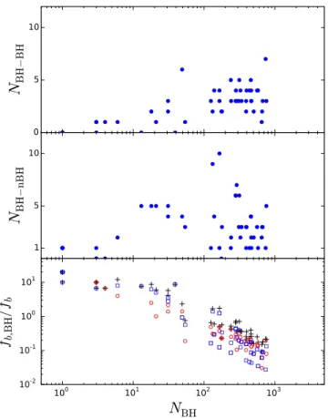
In general, wefind that the number of BBHs (of any kind) in each of our model clusters is much lower compared to the total number of BHs(Table4). Moreover, the BBH numbers are not
strongly dependent on NBH (Figure 11). For example,
depending on the assumptions in our models, wefind a large range in the values of NBH, varying from 0 to 935 at
t=12 Gyr. In contrast, at t=12 Gyr the variation in the numbers of BH–BH (NBH BH- ) and BH–nBH (NBH nBH- )
binaries are 0 to 7 and 0 to 17, respectively. The correlation
Figure 6. Comparison between model clusters S (black), K1 (red), K2 (blue), and K3 (green) (Tables2,3); identical except the assumption for the kick distribution during BH formation. Top-left: evolution of the bound NBHfor the four models. Bottom-left: evolution of rcand rh. Solid and dashed lines denote rcand rh,
respectively. Bottom-right: evolution of rc/rh. To reduce scatter we take running averages for rc/rh. The lines denote the mean and the shaded regions show 1σ spread.
Top-right:final SBPs for the four models. The horizontal and vertical lines denote Sc,obs, rc,obs, and rhl,obsfor each model. Clearly, the bound NBHdepends very
strongly on the assumed distribution of formation kicks for the BHs. As a result, the overall evolution of the cluster also alters dramatically. For example,K1 with
sBH=sNShas only a handful of retained BHs. This cluster evolves to become a dense compact cluster and reaches the binary-burning phase near t=12 Gyr, with an
SBP typical of the so-called core-collapsed observed GCs. In contrast, all other models that retain significantly larger numbers of BHs at t=12 Gyr, evolve very differently.S and K3 keep expanding until t=12 Gyr, whereas model K2 ceases to expand at around t=8 Gyr.
coefficient between NBH and NBH BH- at t=12 Gyr for all
model clusters that did not get disrupted earlier than 12 Gyr is 0.56 and that between NBH and NBH nBH- is 0.07(Table4).
These general trends are understandable from the basic process of how BBHs are created and dynamically processed inside dense star clusters. Almost all primordial binaries containing massive stars are disrupted inside a cluster. This is mainly due to orbital expansion via mass loss, which makes these binaries susceptible to disruption via subsequent strong scattering encounters(Figure12). Thus, most BHs in dense star
clusters are singles. Almost all BBHs in dense star clusters, as
well as BBHs that are ejected from them after t∼102Myr, are binaries that are dynamically created in the dense cores of these clusters, and are not primordial. Note that even if an old star cluster typical of the present-day GCs now appears to have a low central density, its BHs have likely been processed in dramatically higher-density environments as a result of repeated past BH-induced core-collapse episodes (e.g., Figures 1, 3, and 6). Both the values of NBH BH- and
-NBH nBH in a cluster show large fluctuations over time and
can vary between 0 to ∼10 (e.g., Figures 12–15). This is
reflective of the high frequency of dynamical processes that create, modify, disrupt, and eject the BBHs in a dense star cluster, especially during a BH-driven core collapse. In these dense environments BBHs continuously form via three-body
Figure 7. Comparison between models with varying IMFs. Each model has a different α1, where µm-a
dn dm
1for m
å>1M . Black (model S), red (model Is) and
blue(model If) lines denote α1=2.3, 3, and 1.6, respectively (see Section2; Kroupa2001). Left: evolution of the total number of BHs formed (thick lines) and total
number of BHs retained by the cluster(thin lines). Right: evolution of the cluster mass normalized to the initial cluster mass. Starting from otherwise identical initial conditions, the three clusters meet with very different fates. The cluster model with α1=1.6 produces many more BHs compared to other models, expands
enormously, and gets disrupted around t=2 Gyr. The approximate disruption time (Section3.2) is marked by arrows.
Figure 8. Evolution of the star cluster mass normalized by the initial mass of the cluster for models with α1=−1.6. Black, red, and green lines denote
models with our standard kick prescription(models If, WIf), and fallback-independent kick prescriptions with sBH=1 (models IfK1, WIfK1), and 0.01
sNS(models IfK3, WIfK3), respectively. Solid and dashed lines denote
models with strong and weak winds, respectively. All of these clusters are disrupted before t=12 Gyr. In models that retain significant numbers of BHs, weak winds lead to earlier dissolution of the cluster relative to strong winds. Weak winds lead to formation of higher-mass BHs, which lead to faster expansion of the clusters, and correspondingly higher tidal mass loss compared to the strong wind case. For models with sBH=sNS, this is reversed, since in
this case with very low values of NBH, mass loss from stellar evolution and
compact object formation is the dominant effect.
Figure 9. Similar to Figure8, but for modelsK1 (black solid), WK1 (black dashed), IfK1 (red solid), and WIfK1 (red dashed). Since in all models the assumption of sBH=sNS ejects almost all BHs formed in these clusters,
dynamical effects of BHs become unimportant. The dominant effect is from mass loss via compact object formation and immediate ejection of most BHs. In models withα1=1.6, the number of high-mass stars is significantly larger
compared to that in models withα1=2.3. This leads to a much higher mass
encounters, change via swapping of partners in binary-mediated scattering, get disrupted via strong scattering, and get ejected due to recoil from strong scattering encounters(e.g., Heggie1975). The dynamical processes including disruption of
primordial binaries, creation of new ones, and dynamical ejections essentially erase the binary properties the high-mass stars were born with. This in fact is the main difference between BBHs formed in a dense star cluster and BBHs that are born in isolation in thefield. In the latter case, all BBHs are formed from primordial binaries, hence, the BBH properties as well as numbers relative to single stars are directly related to the assumptions of initial binary properties for the high-mass stars.
While large numbers of BHs are still present in a star cluster, the core of the cluster is dominated by the BHs due to mass segregation. Internal dynamics determines how many of these BHs can hold onto their companions once formed via dynamics. As NBH decreases, the BH-driven core collapses
become less pronounced. As a result, a higher fraction of BHs can remain in binaries, and the ejection rate of BBHs decreases. Hence, although NBHdecreases, the fraction of BHs in BH–BH
binaries increases, thus keeping NBH BH- largely unchanged
(Figure 11). On the other hand, while NBH is large, the very
central regions are dominated by the(mostly) single BHs and
lower-mass stars are driven out. A large NBH also keeps the
cluster puffed up, lowering the rate of encounters between BHs and binaries with non-BH members. Only after a cluster is sufficiently depleted of BHs can the rate of formation of BH– nBH binaries, via exchange interactions involving a BH and a binary with non-BH members, increase. However, at this stage the maximumNBH nBH- is likely limited by the low number of
remaining BHs.
The lack of a strong correlation between NBH and NBH nBH
-has some interesting implications. For example, major efforts are now underway to detect BH candidates in GCs (e.g., Strader et al.2012; Chomiuk et al.2013; Strader et al. 2013; Miller-Jones et al. 2014a, 2014b). For detection via
electro-magnetic signals (e.g., by comparing the radio and X-ray luminosities) there must be a BH with a non-BH accreting companion. For simplicity, if we treatNBH nBH- as a proxy for
the absolute upper limit on the number of BH candidates that may be detectable via electromagnetic signatures, the lack of correlation between NBH and NBH nBH- poses a serious
challenge in inferring the number of total BHs in the GC from the discovery of BH candidates in that GC. Note, however, that creation of accreting BHs in star clusters is likely a complex process which requires that the binary is not disrupted for a sufficient time to allow accretion. Even when this is satisfied,
Figure 10. Same as Figure6, but comparing between modelsW (black) and Wrv1fb0.1 (red; Table2). The lower relaxation timescale and average stellar mass for modelWrv1fb0.1 compared to model W lead to faster mass segregation, and as a result faster dynamical processing of BHs. The retained number of BHs NBHin
model clusterWrv1fb0.1 is significantly lower compared to NBHin model clusterW. As a result, model cluster Wrv1fb0.1 ceases to expand by t=12 Gyr, and
begins the relaxation-driven slow-contraction phase. In contrast, model clusterW keeps expanding until the end. Wrv1fb0.1 appears as a higher-density and more compact cluster compared toW.
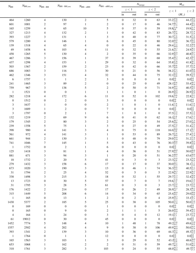
Table 4 Properties of Black Holes
No. NBH NBH,esc NBH BH- NBH BH- ,esc NBH nBH- NBH nBH- ,esc Nmerge Mtot
z<1 z<2 z<1 z<2 in out in out (Me) 1 464 1260 4 130 2 5 0 32 0 63 33.223.847.6 44.224.849.3 2 601 1001 2 97 1 2 0 17 0 46 34.727.546.7 44.428.549.1 3 165 1259 4 65 10 5 0 37 0 59 19.88.821.0 19.910.421.5 4 327 1213 4 132 2 1 0 42 0 83 26.721.830.5 28.722.431.9 5 393 1227 3 131 1 3 0 40 0 77 30.724.037.4 31.524.037.4 6 579 1200 4 146 1 6 0 45 0 80 32.023.644.9 36.724.050.5 7 139 1318 4 65 4 0 0 22 0 46 29.420.037.2 32.221.538.6 8 49 1458 6 103 4 11 0 32 0 55 21.615.734.7 24.915.736.1 9 458 1265 5 130 4 2 0 35 0 66 32.926.746.9 40.827.249.7 10 467 1286 3 156 1 37 0 39 0 68 35.423.548.3 42.321.250.5 11 437 1298 4 153 1 29 0 32 0 64 35.825.947.8 41.8 26.3 50.7 12 503 1367 2 159 2 23 0 42 0 66 35.726.950.8 37.723.951.9 13 686 1083 3 116 3 30 0 21 0 56 38.225.247.1 41.023.050.8 14 462 1346 3 151 4 32 0 44 0 75 32.124.850.9 39.524.352.0 15 6 1757 1 1 2 3 0 0 0 0 0.00.00.0 0.00.00.0 16 241 1465 3 89 2 0 0 25 0 49 28.120.145.6 35.420.449.7 17 759 967 3 138 5 2 0 50 0 71 34.924.649.5 40.524.750.2 18 1 1521 0 0 1 1 1 0 1 0 26.926.926.9 26.926.926.9 19 282 1218 4 172 6 11 0 52 0 102 19.613.429.6 22.814.135.1 20 0 1512 0 2 0 3 0 0 0 0 0.00.00.0 0.00.00.0 21 3 1637 1 0 0 2 1 0 1 0 11.611.611.6 11.611.611.6 22 3 1689 1 2 0 7 0 0 0 0 0.00.00.0 0.00.00.0 23 3 1797 0 2 1 7 1 0 1 0 37.537.537.5 37.537.537.5 24 132 1219 2 69 9 6 0 41 0 62 16.110.721.0 17.611.321.3 25 179 1345 2 80 3 2 0 25 0 54 25.619.030.7 27.020.031.5 26 239 1358 5 75 1 3 0 27 0 49 27.519.337.4 31.4 19.237.5 27 398 980 4 141 3 4 0 75 0 118 16.012.020.0 17.112.120.3 28 561 972 4 141 3 1 0 53 0 89 26.720.031.4 27.421.831.5 29 661 944 2 130 3 1 0 48 0 79 29.021.936.9 31.2 22.7 37.4 30 741 1046 7 145 1 5 0 43 0 76 30.323.748.0 39.824.049.5 31 1 1752 0 2 1 6 0 0 0 0 0.00.00.0 0.00.00.0 32 125 1418 3 81 1 4 0 36 0 51 27.919.348.0 30.0 19.748.6 33 881 671 3 94 3 1 0 20 0 51 36.227.148.0 43.627.750.9 34 18 1732 2 20 5 41 0 3 0 3 23.316.935.9 23.316.935.9 35 279 1432 3 158 6 17 0 17 0 37 30.023.544.1 38.1 23.6 51.1 36 673 1020 3 190 3 13 0 46 1 74 36.323.550.9 40.523.751.1 37 31 1794 2 25 4 52 0 5 0 5 22.916.326.3 22.916.326.3 38 338 1498 3 215 3 18 0 32 1 55 29.721.241.3 32.4 18.450.8 39 13 1723 0 30 5 57 0 7 0 7 19.613.221.9 19.613.221.9 40 31 1795 3 28 5 61 0 3 0 3 23.722.625.9 23.722.625.9 41 176 1422 2 214 0 17 0 26 2 49 26.99.543.2 28.3 11.046.2 42 315 1449 5 208 6 14 0 34 0 65 25.419.346.9 29.019.049.6 43 1 165 0 13 1 2 0 2 0 4 25.923.528.3 33.123.746.7 44 1430 5377 2 185 5 25 0 38 0 105 50.021.853.3 50.0 23.7 53.4 45 0 169 0 0 0 1 0 0 0 0 0.00.00.0 0.00.00.0 46 0 165 0 9 0 2 1 1 1 5 26.025.026.9 39.425.249.3 47 4 164 1 24 0 3 0 4 0 12 19.115.724.7 23.7 15.847.9 48 61 19012 0 30 0 45 0 0 0 0 0.00.00.0 0.00.00.0 49 1452 7774 5 148 4 10 1 48 1 78 49.218.253.8 49.619.953.9 50 1557 2502 4 202 4 9 0 38 0 106 49.946.054.4 50.0 43.4 54.5 51 393 1341 2 139 3 10 0 36 0 69 44.332.055.3 49.332.255.4 52 1 1764 0 1 1 12 0 0 0 0 0.00.00.0 0.00.00.0 53 165 1563 3 103 1 3 0 29 0 52 43.132.063.3 48.6 33.1 58.0 54 653 1068 1 162 2 2 0 31 0 59 49.740.257.2 51.040.558.7 55 310 1761 3 282 3 103 0 24 0 55 48.036.454.2 49.727.374.9
the duty cycle may be low for such accreting binaries(Kalogera et al.2004). We encourage a more detailed study on this topic.
We now focus our attention on understanding the detailed evolution of BBHs inside a cluster and the effects of various initial assumptions through selected example models (Figures 12–15). Since we have shown that the assumed BH
natal kick distribution can bring dramatic changes to the overall cluster evolution, we first investigate the effects of BH formation kicks on the evolution of BBHs that are retained in the cluster(Figure 12). The number of BBHs in the cluster is
quite insensitive to the details of the kick distribution except for the case with sBH=sNS (e.g., model K1). In the high-kick
cases, the large formation kicks essentially eject most of the BHs from the cluster during formation. The natal kicks are also large enough to disrupt all binaries during BH formation. Hence, not surprisingly, in the high-kick models, the values for
-NBH BH as well as NBH nBH- are always low. Interestingly
though, the number of BBHs is low even in our lowest kick models. For example,S, which assumes a fallback-dependent momentum-conserving kick prescription and K3, which assumes that sBH=2.65 km s−1, typically much lower Table 4
(Continued)
No. NBH NBH,esc NBH BH- NBH BH- ,esc NBH nBH- NBH nBH- ,esc Nmerge Mtot
z<1 z<2 z<1 z<2 in out in out (Me) 56 21 1916 1 51 5 160 0 1 0 2 60.260.260.2 67.660.674.6 57 1500 8638 9 248 2 75 0 28 1 94 54.619.156.4 54.857.623.0 58 39 19134 0 43 17 143 0 0 0 0 0.00.00.0 0.00.00.0 59 1917 3554 11 322 4 13 0 14 0 117 77.435.182.0 71.019.884.7 60 54 1469 1 141 3 7 0 33 0 59 33.630.345.7 36.230.451.4 61 1 1519 0 1 1 25 3 0 3 1 68.359.774.6 71.659.979.5 62 289 1237 3 175 7 10 0 31 0 69 34.324.343.0 36.227.548.3
Note. Serial numbers for models are the same as in Table2. Columns“in” and “out” denote BH–BH mergers inside and outside clusters. Number of BH–BH mergers and their total masses in the source frame are listed for z<1 and z<2 assuming z=0≡t=12 Gyr. The median and 2σ ranges in total mass are listed.
Figure 11. Top: the number of bound BHs NBHvs. the number of bound BH–
BH binariesNBH BH- . Middle: NBHvs. the number of bound BH–nBH binaries
-NBH nBH. Bottom: binary fraction in BHs( fb,BH) normalized by the overall
binary fraction fb. Pluses(black), circles (red), and squares (blue) denote the
normalized binary fraction for all BH binaries, BH–BH binaries, and BH–nBH binaries, respectively. A larger fraction of BHs are in binaries relative to the overall binary fraction for models with low NBH. High NBHleads to BH-driven
core collapse which typically disrupts and ejects BH binaries. As NBH
decreases, BH-driven core-collapses stop occurring, reducing the efficiency of BBH destruction and ejection. BHs being the most massive objects, typically get exchanged into binaries via binary-mediated scattering encounters. As a result, the fraction of BHs in binaries increases as NBHdecreases.
Figure 12. Evolution of the number of binary BHs bound to the cluster for different assumed natal kick distributions for BHs. Top and bottom panels show BH–BH and BH–nBH binary numbers. Both NBH BH- and NBH nBH
-show large scatters over time. This is a direct consequence of the continuous disruption and ejection of existing binaries and dynamical formation of new ones at any given time in clusters. To reduce scatter we have under-sampled and show the mean (lines) and±one standard deviation (shaded region). Black, red, blue, and green denote modelsS, K1, K2, and K3, respectively (Table2). BothNBH BH- andNBH nBH- remain low independent of the assumed
distribution of natal kicks for BHs. This indicates that the softening of orbits for massive binaries due to mass loss via winds and compact object formation is responsible for dynamical disruption of most primordial binary orbits, and that this process does not depend on the natal kick distribution. Even with very low adopted natal kicks for BHs, sBH=2.65 km s−1,K3 contains low numbers of