Thermal performance modeling of complex fenestration systems

Publisher’s version / Version de l'éditeur:

Journal of Building Performance Simulation, 2, 3, pp. 189-207, 2009-09-01

READ THESE TERMS AND CONDITIONS CAREFULLY BEFORE USING THIS WEBSITE. https://nrc-publications.canada.ca/eng/copyright

Vous avez des questions? Nous pouvons vous aider. Pour communiquer directement avec un auteur, consultez la

première page de la revue dans laquelle son article a été publié afin de trouver ses coordonnées. Si vous n’arrivez pas à les repérer, communiquez avec nous à PublicationsArchive-ArchivesPublications@nrc-cnrc.gc.ca.

Questions? Contact the NRC Publications Archive team at

PublicationsArchive-ArchivesPublications@nrc-cnrc.gc.ca. If you wish to email the authors directly, please see the first page of the publication for their contact information.

NRC Publications Archive

Archives des publications du CNRC

This publication could be one of several versions: author’s original, accepted manuscript or the publisher’s version. / La version de cette publication peut être l’une des suivantes : la version prépublication de l’auteur, la version acceptée du manuscrit ou la version de l’éditeur.

For the publisher’s version, please access the DOI link below./ Pour consulter la version de l’éditeur, utilisez le lien DOI ci-dessous.

https://doi.org/10.1080/19401490903046785

Access and use of this website and the material on it are subject to the Terms and Conditions set forth at

Thermal performance modeling of complex fenestration systems Laouadi, A.

https://publications-cnrc.canada.ca/fra/droits

L’accès à ce site Web et l’utilisation de son contenu sont assujettis aux conditions présentées dans le site LISEZ CES CONDITIONS ATTENTIVEMENT AVANT D’UTILISER CE SITE WEB.

NRC Publications Record / Notice d'Archives des publications de CNRC: https://nrc-publications.canada.ca/eng/view/object/?id=6fa429e5-c075-4324-876f-1620192de892 https://publications-cnrc.canada.ca/fra/voir/objet/?id=6fa429e5-c075-4324-876f-1620192de892

http://www.nrc-cnrc.gc.ca/irc

T he r m a l pe rfor m a nc e m ode ling

of c om plex fe ne st rat ion

syst e m s

N R C C - 5 0 8 6 6 #

L a o u a d i , A .

S e p t . 1 , 2 0 0 9

A version of this document is published in / Une version de ce document se trouve dans:

Building Performance Simulation, 2, (3), pp. 189-207, September 01, 2009 DOI: http://dx.doi.org/10.1080/19401490903046785

The material in this document is covered by the provisions of the Copyright Act, by Canadian laws, policies, regulations and international agreements. Such provisions serve to identify the information source and, in specific instances, to prohibit reproduction of materials without written permission. For more information visit http://laws.justice.gc.ca/en/showtdm/cs/C-42

Les renseignements dans ce document sont protégés par la Loi sur le droit d'auteur, par les lois, les politiques et les règlements du Canada et des accords internationaux. Ces dispositions permettent d'identifier la source de l'information et, dans certains cas, d'interdire la copie de documents sans permission écrite. Pour obtenir de plus amples renseignements : http://lois.justice.gc.ca/fr/showtdm/cs/C-42

THERMAL PERFORMANCE MODELING OF COMPLEX FENESTRATION SYSTEMS A. LAOUADI, PH.D., ASHRAE MEMBER

INSTITUTE FOR RESEARCH IN CONSTRUCTION,NATIONAL RESEARCH COUNCIL OF CANADA 1200MONTREAL ROAD,BUILDING M-24,OTTAWA,ONTARIO,CANADA K1A0R6 TEL.: (613)9906868. FAX: (613)9543733. EMAIL:AZIZ.LAOUADI@NRC-CNRC.GC.CA

ABSTRACT

Complex fenestration systems (CFS) have become standard elements in façade design of high performance buildings. They include, for example, shadings devices to control illumination, solar heat gains, glare, and view-out, and photovoltaic elements imbedded in glazing layers to produce electrical energy on site. However, current methodologies to evaluate the thermal performance of CFS are limited to a few products and types. This paper

develops a general methodology to compute the thermal performance of CFS. The methodology assumes each system layer as porous with calculated

effective radiation and thermal properties. A new thermal penetration length model was developed to account for the effects of porous layers on the convective film coefficients of adjacent gas spaces, and applied to various types of shading devices. This methodology is validated using the available measurement and CFD simulation results for the U-factor of double-glazed windows with between-pane and internal blinds.

KEYWORDS

NOMONCLATURE

AB : solar absorptance (decimals)

C : constant, equation (16) (dimensionless) c : specific heat (J/kg.K)

D : constant, equation (17) (dimensionless) E : black body emissive power (W/m2) F : form factor (dimensionless)

Fr : fullness ratio of drapes (dimensionless) g : gravitational coefficient (m/s2)

H : characteristic plate height (m)

h : convective film coefficient of gas space (W/m2K) k : thermal conductivity (W/mK)

L : thickness (m)

m : constant, equation (16) (dimensionless) Nu : Nusselt number (dimensionless)

q : radiative flux density (W/m2) Ra : Rayleigh number (dimensionless) RF : solar reflectance (decimals)

s : spacing of slats, or length of drapery pleats (m) SR : surface area ratio (decimals)

T : temperature (K)

TR : solar transmittance (decimals) v : gas velocity (m/s)

w : width of cavity, or slat (m) z : height of cavity (m)

Δx : thickness of a nodal control volume (m) SUBSCRIPTS

a : gas space, or average b : back surface, or blind layer beam : beam solar radiation

c : convection d : diffuse

dif : diffuse solar radiation e : emission

eff : effective eq : equivalent f : front surface

i : layer node index, or incident j : layer index m : material o : outgoing r : radiation s : screen layer sol : solar sm : slat material GREEK SYMBOLS

α : slat angle (radians), or gas diffusivity (m2/s), or absorption coefficient per unit length (m-1)

β : inclination angle (radians), or expansion coefficient of gas (K-1) δ : reduced thermal penetration length (m)

ε : emissivity (decimals), or emissivity coefficient per unit length (m-1) γ : thermal penetration length of a porous layer (m)

κ : fibre density (dimensionless)

ηPV : photovoltaic cell efficiency (decimals)

ρ : density (kg/m3), or long wave reflectance (decimals) τ : long wave transmittance (decimals)

υ : gas viscosity (m2/s)

ϕ : openness factor (decimals) ω : porosity (decimals)

1 INTRODUCTION

Complex fenestration systems have become standard components in high performance building designs. CFS include, for example, varying types of shadings devices integrated between glazing layers, or attached to the interior or exterior glazed façades to control natural illumination, solar heat gains, and view out, and photovoltaic elements imbedded in glazing layers to produce electrical energy on site. In some building applications with high indoor moisture contents such as restaurants and swimming pools, electrical-conductor transparent thin films are applied to indoor window surfaces to control moisture condensation and maintain view-out, and provide local secondary space heating. Although there has been significant advancement in the performance evaluation of CFS, predictions of the thermal performance of CFS remain a challenge to be addressed, particularly for systems with shading devices.

In the past decades, there has been significant work devoted to the evaluation of the optical, daylighting and energy performance of CFS incorporating

shading devices. The ISO 15099 standard (ISO, 2003) presents a validated model to compute the optical and long-wave radiation characteristics of slat-type blinds. Other blind related work carried out further validation studies and developed improvement to the ISO blind model to account for the slat

thickness, curvature and specularity (Rosenfeld et al., 2000; Breitenbach et al., 2001; Chantrasrisalai and Fisher, 2006; Collins and Jiang, 2008; Yohoda and Wright, 2005; 2004b). The IEA Task 27 (Kohl, 2006) carried out a comprehensive assessment of the solar optical and thermal performance of several product types of interior and exterior blinds and roller shades through measurement and computer simulation using the ISO 15099 standard and simple models. The IEA Task 34/43 (Loutzenhiser et al., 2007) carried out empirical validations of building-energy simulation tools for daylighting performance and thermal loads of interior and exterior Venetian blinds and shading screens. Most of the tested simulation tools used simple models for the prediction of the optical and thermal performance of the tested shading

devices. Recent work under the ASHRAE project (RP 1311) carried out experimental studies and developed semi-empirical optical models for several types of shading devices, including drapes, roller blinds and insect screens (Kotey et al., 2009a,b).

However, predictions of the thermal performance of CFS (e.g., U-factor) are at the early stage, particularly those related to the convection flows in open gas cavities adjacent to porous layers. Porous layers are transparent to thermal radiation, and permeable to fluid flow through their structure. Work under this area can be divided into four main approaches, namely: simple models, empirical-based models, CFD-based models, and a mix of models.

Simple thermal models of CFS are based on the thermal-resistance approach developed for simple fenestration systems, made up of essentially plain opaque glazing (Yahoda and Wright, 2004a; Wright, 2008). A

one-dimensional conduction heat transfer model is used for glazing layers coupled with radiation and convection models at the layer boundary surfaces.

Convection models use existing correlations for the convective film

coefficients in enclosed gas cavities or around tilted flat surfaces. Complex layers such as shading devices are treated as individual layers with effective radiation properties (emissivity and infra-red transmittance), but with assumed uniform layer temperature (no thermal resistance of shading layer). These simple models have been implemented in currently available fenestration tools such as WINDOW (LBNL, 2008) and WIS (WinDat, 2008). Recent research showed, however, that these simple models were not accurate for slat-type blinds (Yahoda and Wright, 2004a), and for diathermanous –

thermally transparent- layers (Collins and Wright, 2006). Furthermore, these models cannot be applied to CFS layers with significant radiation absorption and emission within their media, such as, for example, shading devices and transparent or translucent insulation. In addition, these models do not account for energy production (e.g., electrical resistance heating) and conversion (e.g., photovoltaic) within layer media, which are getting more popular in today’s building design.

Given the limitations of the simple thermal-resistance models, extensive work has been devoted to the experimental performance evaluation of CFS, and investigation of fluid flows in cavities of CFS incorporating shading devices. Earlier work by Grasso and Buchanan (1979) and Grasso et al. (1990) conducted measurement using the guarded hot plate method of the U-factor of single glazed windows combined with several product types of interior draperies and roller shadings. They found that sealing the cavities between shadings and window had significant effects in reducing the U-factor of windows. Fang (2000, 2001) conducted measurement using the hotbox method of the U-factor of single and double-glazed windows with interior curtains and Venetian blinds. Empirical relationships derived from the experiments were also developed for the U-factor of similar window and

shade configurations. Garnet (1999) and Huang (2005) conducted laboratory measurement using the guarded heated plate apparatus of the U-factor of regular and low-e double-glazed windows with between pane metallic

Venetian blinds. They found that the slat-tip-to-glazing spacing and slat angle positions had significant effect on the U-value of the window and blind system. The thermal bridging effect of the metallic blinds reached its maximum when the slat angles were horizontal, where the U-factor was higher than when slats were closed. To understand how the fluid flow behaves in cavities between window glazing and shadings, Machin et al. (1998), Collins et al. (2002b), and Naylor and Lai (2007) conducted interferometric experiments to visualize the temperature and air flow patterns in double glazed windows with internal and between pane metallic Venetian blinds. The local Nusselt

number along the window height was measured for varying slat-tip-to-window glazing spacing. Cellular flows within cavities between slats were observed, particularly for low slat angle positions near the horizontal. Gas mass transfer through the blind layer was also observed. The studies concluded that the thermal conductivity of blinds and radiation heat transfer had strong effects on the local Nusselt number.

Parallel to the above experimental investigations, CFD computer simulations have been used for varying purposes: (1) to investigate the flow and

temperature patterns in gas cavities between glazing and shading layers, (2) to validate the simulation results with the measurement, and (3) to develop useful correlations for the convective film coefficient in cavities between glazing and shading layers. Laminar, two-dimensional flows were generally considered in the investigated work. Convective flows with and without direct radiation coupling in windows with internal Venetian blinds were addressed by several researchers, including Ye et al. (1999), Phillips et al. (2001), Collins et al. (2002a), Collins (2004), Shahid and Naylor (2005), and Naylor et al.

(2006). The maximum effect of blinds on the heat transfer through the

window and blind system was found when the blinds were closed, and placed near to the window glazing. The obtained simulation results for the

temperature and flow patterns compared favourably with the available

measurement of similar window and blind configurations. Correlations for the average Nusselt number of the window-blind cavity were also developed for various slat angles. Naylor and Collins (2005), Avedissian (2006), and Avedissian and Naylor (2007) addressed windows with between-pane

Venetian blinds. Naylor and Collins (2005) employed a full CFD model (with direct radiation coupling) to simulate the experimental configuration of Garnet (1999). Overall, good comparison results were obtained. Avedissian (2006) employed a convection-only CFD model, and covered a broad range of flow governing parameters, including low and high values of the blind thermal conductivity, and glazing-to-blind spacing. Correlations for the average Nusselt number of the window cavity were developed for various slat angle positions. When the radiative heat transfer was post-coupled with the convective heat transfer, the obtained result for the U-factor of window compared favourably with the experimental results of Huang (2005).

Avedissian and Naylor (2007), on the other hand, employed a full CFD model, and obtained comparable results with those of Avedissian (2007) and Huang (2005).

The CFD-based correlations for the convective film coefficient of cavities between glazing and shading layers have been successfully used in the thermal-resistance models as stated previously. Shahid (2003), Shahid and

Nayler (2005), and Nayler et al. (2006) applied this approach to windows with internal blinds, and Naylor and Collins (2005) and Avedissian and Naylor (2007) to windows with between-pane blinds. They found that the predictions of the U-factor of windows using such improved models compared well with the full CFD simulation, and deviated from the available measurement by about 10%. Recently, Wright et al. (2008) developed a simplified model to compute the film coefficient of a double glazed window cavity with between-pane metallic blinds. The blinds divide the window cavity into two sub cavities. Wright et al. (2008) used the existing cavity correlations (similar to those included in the ISO 15099 standard) to compute the film coefficients of the sub cavities based on a modified sub cavity width. The latter, which is larger than the true sub cavity width (equal to slat tip-to-glazing spacing), was found proportional to the slat width and cosine angle. The proportionality constant was determined by comparing the model predictions of U-factor with the measurement results of Huang (2005). The proposed model yielded exceptional results for the window cavity spacings of 17.78 mm and 25.4 mm. However, the model failed to accurately-predict the U-value of the window with the larger cavity spacing of 40 mm. Despite this drawback, the model of Wright et al. (2008) indicates an important conclusion that existing

correlations for cavity film coefficients may be safely used to predict the thermal performance of window and shade systems without resorting to the time-consuming and computationally intensive CFD simulation. Furthermore, the model of Wright et al. (2008) allows more flexibility to address other

combinations of shading types and tilted window configurations. Future work should address improvement to the model of Wright et al. (2008) for general applications.

It should be noted that the current advanced empirical and CFD-based thermal models are limited to single or double glazed windows with specific metallic blinds. They do not account for other physical and thermal properties of blinds such as slat spacing and thermal conductivity. Furthermore, they cannot be applied to other types of shading devices such as drapes, or to other window tilt configurations.

This paper addresses some of the previously identified issues in the thermal modelling of CFS. The aim is to develop a general methodology to compute the thermal performance of complex fenestration systems for implementation in fenestration computer programs.

2 OBJECTIVES

The specific objectives are:

• To revisit the current models of the heat transfer mechanisms through fenestration layers, and include the peculiarities of CFS such as imbedded elements for energy production or conversion, permeable layers for mass and radiation, and open gas spaces.

• To develop models to compute the effective radiation and thermal properties of permeable layers.

• To develop models to compute the convection film coefficients of gas spaces adjacent to porous layers.

• To validate and assess the methodology by comparing its predictions with the available measurement and simulation data.

3 OVERVIEW OF EXISTING FENESTRATION MODELS

Fenestration systems have undergone significant innovation, from simple systems, made up of essentially plain glass layers and enclosed sealed gas cavities, to far more complex systems. The latter may embody complex glazing layers with applied films, and shading devices with complex

geometries. Heat transfer in such complex systems has, therefore, become more complex to handle. Glazing layers may be permeable to mass and thermal radiation, and cavity spaces may be sealed, or open so that cavity gas can move from one space to another through permeable layers, or through deliberate cavity openings. The flow in the cavity space may be forced (e.g., wind-driven), or natural, driven by buoyancy forces and

temperature gradients (stack effect). The current methodology to compute the thermal performance of complex fenestration systems has, unfortunately,

inherited the methodology and assumptions of the simple fenestration systems. As outlined in the ISO 15099 standard (ISO, 2003), the current methodology treats glazing layers as thermally opaque layers, except in the thermal radiation energy balance where layers may be thermally transparent. Thermal radiation transport within a complex layer medium is not accounted for. Models for the convective heat transfer use existing correlations for heat transfer in sealed gas cavities, or around tilted flat surfaces. Correlations for the convective heat transfer in open cavities with permeable (porous) layers are not available. The ISO 15099 standard provides, however, a simple algorithm to calculate the convection film coefficient of a ventilated open cavity based on the film coefficient of a sealed cavity (hcavity) and the average gas velocity (vj) in cavity space. For buoyancy-driven flows, the gas velocity is calculated based on the piston flow model and the total pressure difference between the gas space and its connected environment. The film coefficient of a gas space (j) is, thus, given by the following relation:

j j cavity j c h h _, =2⋅ _, +4⋅v (1)

The ISO 15099 standard also suggests using equation (1) for forced cavity flows with known velocities.

Equation (1) was developed particularly for one-way cavity flows based on empirical and numerical data (Dick and Oversloot, 2003). Recent research also found that equation (1) yielded comparable results to the experimental and numerical data for mechanically ventilated double skin facades (Corgnati et al., 2007). However, care should be exercised when applying the equation for cavities where two-way flows might occur (Manz et al., 2004).

Regarding the estimation of the cavity film coefficient (hcavity), there are several proposed methods, particularly, for glazing cavities encompassing slat-type blinds. The ISO 15099 model assumes the blinds divide the glazing cavity into two sub cavities and the cavity film coefficient is evaluated based on the width of the sub cavity (half of the glazing cavity if the blinds are placed in the center). This model does not account for the slat angle position and

geometrical characteristics. Other models use the slat-tip-to-glazing width to evaluate the cavity film coefficient. However, when compared with the experimental and CFD simulation data, these two models were found to underestimate or overestimate the thermal transmittance (U-factor) of windows (Yahoda and Wright, 2004a; Wright et al., 2008). Wright et al. (2008) recently proposed an improved model, termed the reduced-slat-width (RSW) model, in which the slat-tip to glazing width is calculated based on a 70% reduced slat width (0.7w). This model does not take into account the spacing and thermal conductivity of slats.

It should be added that there are no guidelines on how to apply the ISO ventilated cavity model for sealed glazing cavities encompassing porous shadings or slat-type blinds, despite the fact that most of the experimental work listed in this paper showed that there was a significant air flow through blind layers, particularly at the top and bottom edge sections, even when blinds are fully (but not ideally) closed (Naylor and Lai, 2007).

4 THE PROPOSED METHODOLOGY

The following sections present the details of a new methodology to compute the thermal performance of complex fenestration systems. The methodology starts by laying down the underlying equations for the heat transfer through complex glazing layers, and develops appropriate methods to handle the convective and radiative heat transfer in open cavities with layers permeable to radiation and mass.

4.1 ASSUMPTIONS

The following assumptions are considered.

• Each glazing layer is assumed solid and porous with calculated effective radiation and thermal properties to account for any convection and radiation effect in a layer medium.

• Heat transfer through a glazing layer medium is by one-dimensional conduction.

4.2 LAYER HEAT TRANSFER

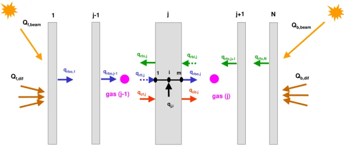
Consider a multi-layer fenestration system consisting of (N) layers as shown in Figure 1. Layer 1 faces the exterior environment and layer (N) faces the interior environment. Each layer (j) is surrounded by gaseous spaces at its boundary surfaces. The layer exchanges heat with the adjacent

environments by convection to the gaseous spaces and radiation to the adjacent layers. Heat is transported through the layer by conduction, and radiation. The transient energy balance on an elemental control volume at node (i) within a layer (j) is expressed by the following relation (Siegel and Howell, 2002): i j i j sol i j r j i j i j i j i j q q q x T k x t T c , ,, , , 0,, , , , ⎟⎟+ + ⎠ ⎞ ⎜⎜ ⎝ ⎛ − ∂ ∂ ∂ ∂ = ∂ ∂ ρ (2) where:

cj,i : effective specific heat at node i of layer j (J/kg.K)

kj,i : effective thermal conductivity at node i of layer j (W/mK) Tj,i : temperature at node i of layer j (K)

qr,j,i : net radiation flux per unit surface area at node i of layer j (W/m2) qsol,j,i : absorbed solar radiation per unit volume at node i of layer j (W/m3) q0,j,i : heat generation per unit volume at node i of layer j (W/m3)

ρj,i : effective density at node i of layer j (kg/m3)

If the front (facing the exterior environment) and back (facing the interior environment) surfaces of layer j are both subject to the beam and diffuse incident solar radiation, the absorbed solar heat per unit volume at node i is expressed as follows: i j sol b i j sol f i j sol q q q _{, ,} = _{, ,,} + _{, , ,} (3) with:

(

fbeam fdif

)

j f i j f PV PV dif f i j d f beam f i j f i j sol f q q SR TR q q q_{, , ,} =α _{, ,} ⋅ _, +α _{, , ,} ⋅ _, − ⋅η _{,, ,} ⋅ _{,1: −1 ,} + _, (4)

(

bbeam bdif

)

j N b i j b PV PV dif b i j d b beam b i j b i j sol b q q SR TR q q q _{, , ,} =α _{, ,} ⋅ _, +α _{, ,,} ⋅ _, − ⋅η _{, , ,} ⋅ _{, : +1 ,} + _, (5) where:

qf,beam : beam solar radiation flux density incident on the front surface of fenestration system (W/m2)

qb,beam : beam solar radiation flux density incident on the back surface of fenestration system (W/m2)

qf,dif : diffuse solar radiation flux density incident on the front surface of fenestration system (W/m2)

qb,dif : diffuse solar radiation flux density incident on the back surface of fenestration system (W/m2)

SRPV : ratio of photovoltaic surface area to layer surface area (decimals) TRf,1:j-1 : front solar transmittance of layer stack 1 to j-1 (decimals) TRb,N:j+1 : back solar transmittance of layer stack N to j+1 (decimals) αf,j,i : absorption coefficient per unit length of layer j at node i for the front incident beam solar radiation (m-1)

αb,j,i : absorption coefficient per unit length of layer j at node i for the back incident beam solar radiation (m-1)

αf,d,j,i : absorption coefficient per unit length of layer j at node i for the front incident diffuse solar radiation (m-1)

αb,d,j,i : absorption coefficient per unit length of layer j at node i for the back incident diffuse solar radiation (m-1)

ηPV,f,j,i : photovoltaic cell efficiency of layer j at node i to convert the front incident solar energy into electric energy (decimals)

ηPV,b,j,i : photovoltaic cell efficiency of layer j at node i to convert the back incident solar energy into electric energy (decimals)

The intermediate stack transmittance values in equations (4) and (5) are usually not standard outputs of a fenestration calculation program. However, they can be determined based on the standard outputs for the layer

absorptances and fenestration system reflectances as follows:

∑

− = − = − − 1 1 , 1 : 1 , 1 j k k f f j f RF AB TR (6)

∑

+ = + = − − 1 , 1 : , 1 j N k k b b j N b RF AB TR (7) where:

ABf,j : front solar absorptance of layer j (decimals) ABb,j : back solar absorptance of layer j (decimals)

RFf : front solar reflectance of fenestration system (decimals) RFb : back solar reflectance of fenestration system (decimals)

The nodal solar absorption coefficients (αj,i) may be calculated based on the layer solar absorptance (ABj). In the absence of a photovoltaic energy conversion, one may assume that the solar radiation is uniformly absorbed along the layer thickness (Lj). In this case, the nodal solar absorptance coefficients are equal to the layer solar absorptance divided by its thickness (αj,i = ABj/Lj). However, if the photovoltaic energy conversion is present, one may assume that the solar energy is absorbed only at the photovoltaic cell layers. In this case, the nodal absorptance coefficients are zero, except at the photovoltaic cells nodes. The nodal solar absorptance coefficient at the photovoltaic cell node is then equal to the layer solar absorptance divided by the total thickness of the nodal control volumes enclosing the photovoltaic layers (αj,i = ABj/∑ΔxPV,cell). For layers opaque to the solar radiation, the solar radiation is absorbed at the boundary surfaces. The nodal absorptance

coefficients are therefore zero, except at the boundary nodes where they are equal to the layer solar absorptance divided by the thickness (Δxj,i) of a hypothetical control volume adjacent to the boundary surface (αj,i = ABj/Δxj,i). The net radiation flux (qr) is a complex quantity to calculate. It relates to the emission and absorption of thermal radiation within a layer medium. One detailed approach is to formulate the net radiation flux based on the radiation intensity distribution within a layer medium. This requires solving additional partial differential equations for the radiation transport in the medium (Siegel and Howell, 2002). This approach is possible, in particular, for media whose radiation properties (emission, absorption and scattering coefficients) and geometrical details are known. Another approach, which is well suited to complex fenestration systems, is to formulate the nodal net radiation flux in terms of the effective emissivity and absorptivity coefficients of a layer medium, its nodal emissive power and the incident radiation from all directions. In this approach, the layer medium is assigned nodal effective emissivity and absorptivity coefficients, which may be pre-calculated based on a detailed radiation model for the layer medium. The effective emissivity coefficients indicate the portion of the black body energy emitted per unit length, which exits from the layer boundary surfaces. Similarly, the nodal effective absorptivity coefficients indicate the portion of absorbed energy per unit length of radiation incident on the layer boundary surfaces. By virtue of the Kirchhoff’s law (Siegel and Howell, 2002), the effective absorptivity and emissivity coefficients are equal. The effective radiation properties depend on the medium geometrical details, and may vary along the layer thickness. In this approach, the gradient of the radiation flux density is expressed as follows:

(

f ji bji

)

ji j rbi i j b j rfi i j f i j r E q q x q , , , , , , , , , , , , , _{=ε ⋅ +ε ⋅ − ε +ε ⋅} ∂ ∂ − (8) where:

qrfi,j : radiation flux density incident on the front surface of layer j given by equation (13) (W/m2)

qrbi,j : radiation flux density incident on the back surface of layer j given by equation (13) (W/m2)

εf,j,i : front effective emissivity coefficient per unit length at node i of layer j (m-1)

εb,j,i : back effective emissivity coefficient per unit length at node i of layer j (m-1)

The nodal emissivity (absorptivity) coefficients may be calculated based on the effective emissivities of a layer (εeff,j), which themselves may be available for layers with known geometrical details such as slat-type blind layers (ISO, 2003; Yahoda et al., 2004b), or screen type layers or drapes (see equations 21 to 23, and 32 to 33 ). For layers, which are fully transparent to thermal radiation, the emission and absorption of thermal radiation may occur along the layer thickness. In this case, the nodal emissivity coefficients may be assumed equal to the layer effective emissivity divided by its thickness (εj,i = εeff,j /Li). For layers, which are weakly transparent or opaque to thermal radiation, the emission and absorption may be assumed to occur at the layer boundary surfaces. The nodal emissivity coefficients are, therefore, zero, except at the boundary nodes where they are equal to the layer effective emissivity divided by the thickness (Δxj,i) of a hypothetical control volume adjacent to the boundary surface (εj,i = εeff,j/Δxj,i).

To solve equation (2), the boundary node temperatures at i = 1 and j = m have to be given. Applying the energy balance to a control volume

encompassing the boundary nodes, one may obtain the following equations:

( )

(

)

1 1 , , 1 , , 0 1 , , 1 , 1 , 1 , 1 , 1 , 1 1 , 1 , x x q q q T T h x T k x t T c _j j _j j _{cj aj j sol j j} r j _⎟⎟Δ ⎠ ⎞ ⎜⎜ ⎝ ⎛ ∂ ∂ − + + − + ∂ ∂ = Δ ∂ ∂ ρ _{− −} (9)

( )

(

)

m m j r m j m j sol m j j a j c m j m j m m j m j x x q q q T T h x T k x t T c _⎟⎟Δ ⎠ ⎞ ⎜⎜ ⎝ ⎛ ∂ ∂ − + + − + ∂ ∂ − = Δ ∂ ∂ ρ , , , , 0 , , , , , , , , , (10) where:

hc,j-1 : convection film coefficient of gas space (j) (W/m2K) hc,j : convection film coefficient of gas space (j-1) (W/m2K) Ta,j-1 : average temperature of gas space (j-1) (K)

Ta,j : average temperature of gas space (j) (K)

Δxj,1 : thickness of a control volume at boundary node i=1 of layer j (m) Δxj,m : thickness of a control volume at boundary node i=m of layer j (m) Equations (2), (9) and (10) are non-linear and cannot be solved analytically. A suitable numerical method should therefore be used.

4.3 RADIATIVE HEAT TRANSFER

As previously mentioned in the assumptions, each layer is characterized by the effective radiation properties for transmittance (τeff), reflectance (ρeff), and emissivity or absorptance (εeff). Layers are assumed long enough so that the radiative contribution from the edge spacer sections can be neglected. This assumption holds for most fenestration systems, particularly when the calculation of the centre-glazing thermal conductance (or U-factor) is

concerned. However, this assumption may break down in certain applications of double-skin facade systems where the order of magnitude of the thickness of the enclosed air spaces may be comparable to the layer lengths. In this case, a three surface (two layers and edge spacer section) radiative transfer should be considered together with a proper heat balance of the spacer sections.

Consider an isolated layer (j) as shown in Figure 1. The outgoing radiative fluxes from the front and back surfaces of layer are expressed as follows:

j ef j rfi j f eff j rbi j b eff j rfo q q q q _, =τ _{, ,} ⋅ _, +ρ _{, , ,} + _, (11)

j eb j rbi j b eff j rfi j f eff j rbo q q q q , =τ , , ⋅ , +ρ , , , + , (12)

The incident radiative fluxes on the front and back surfaces of layer are expressed as follows: 1 , , 1 ,

,j = rfoj+ ; rfi j = rboj−

rbi q q q

q (13)

where:

qef,j : emitted radiative flux density of layer (j) exiting from its front surface (W/m2)

qeb,j : emitted radiative flux density of layer (j) exiting from its back surface (W/m2)

qrfo,j : radiative flux density exiting from the front surface of layer (j) (W/m2) qrbo,j : radiative flux density exiting from the back surface of layer (j) (W/m2) qrfi,j : radiative flux density incident on the front surface of layer (j) (W/m2) qrbi,j : radiative flux density incident on the back surface of layer (j) (W/m2)

Note that the environment radiative fluxes qrbo,j=0 and qrfo,j=N+1 denote the incident fluxes from the exterior and interior environments, respectively. The emitted radiative fluxes of the layer include the emission of radiation from the bulk layer medium. In a discrete nodal representation of the layer

medium, the emission radiative fluxes are given by the following relations:

∑

∫

ε ⋅ ⋅ = =₌ ε ⋅Δ ⋅ = i m i i j i i j f L j j f j ef x E x dx x E q j 1 , , , , , ( ) ( ) (14)

∑

∫

ε ⋅ ⋅ = =₌ ε ⋅Δ ⋅ = i m i i j i i j b L j j b j eb x E x dx x E q j 1 , , , , , ( ) ( ) (15)

Equations (11) and (12) may be solved using a sequential iterative procedure, in which equation (11) is solved first for all layers (j = 1 to N), followed by equation (12). The process is repeated until convergence is reached.

Convergence is declared if the relative change in the nodal temperatures is less than a tolerance value.

4.4 CONVECTIVE HEAT TRANSFER IN OPEN GAS CAVITIES

A gas cavity between two consecutive layers is said to be open if one of the layers is permeable to gas, or/and one of the edges is deliberately un-sealed at the top, bottom or side surfaces. As mentioned before, the convective heat transfer in open cavities with layers permeable to radiation and mass is a complex phenomenon to predict as the convective effect of the gas cavity may extend to the media of the permeable layers and to other adjacent cavity spaces. To isolate the effect of the convective and radiative heat transfer in a layer medium from the convective heat transfer occurring in the adjacent gas space, each glazing layer is assumed to behave as a porous medium having equivalent effective radiation and thermal properties. The latter should be calculated for a given layer type. This assumption provided acceptable

results for flows in air gaps encompassing shading devices (Safer et al., 2005; Zhang et al. 1991). The convective heat transfer in the gas cavity may be by natural or forced convection, or a combination of the two. In all cases, the model of the ISO standard 15099 for ventilated cavities (equation 1) is used in this work, but with a proper calculation of the cavity film coefficient (hcavity) and gas velocity (v). The following sections present new models to compute these quantities (hcavity and v) for open cavities bounded by porous layers.

4.4.1 Thermal Penetration Length Model For Natural Convection

The thermal penetration length model is used to compute the film coefficient of a gas cavity (hcavity) enclosed between porous layers and subject to

buoyancy driven flows. The thermal penetration length model stems from the fact that if natural convection is occurring in a cavity gas space, the

convective effect may penetrate the porous layers up to a certain length (or depth). This phenomenon is known as penetrative convection, particularly in porous media (Bejan, 2004). For convective flows around surfaces, the thermal penetration length is equivalent to the thickness of the boundary layer as the latter separates between two zones: boundary layer zone with

significant temperature gradient and a stagnant zone far away from the surface. The convective heat transfer from the bounding layers to the cavity gas space is, therefore, a function of this thermal penetration length (Bejan, 2004).

To apply this concept to the problem of heat transfer in complex fenestration systems, consider a porous layer (j) of thickness Lp, forming a gas cavity with an adjacent layer (j+1). The layer (j) is initially at a uniform temperature Tj. If the adjacent layer (j+1) is maintained at a different temperature Tj+1, a

buoyancy-induced flow may occur in the cavity, and the thermal convection effect may penetrate the medium of layer (j) up to a distance γ (see Figure 2). This convection effect may invalidate the use of correlations for cavity film coefficient based on the cavity thickness Lj. As the convective heat transfer in the gas cavity is a function of this penetration length (γ), one may, therefore, postulate that the cavity film coefficient (hcavity) may be obtained using the existing correlations applied on a hypothetical cavity with a thickness linearly proportional to the thermal penetration length, namely Lj + δ (with δ ∝ γ). The thermal penetration length (γ), which is solely due to convection, depends on the geometrical and thermal characteristics of the layer medium (j), and the temperature difference (Tj+1 - Tj). It should, however, be independent of the cavity spacing Lj. For highly porous layers such as shading layers (e.g., porosity ≈ 0.98 for blinds and draperies), convection in the cavities of the porous layer may be considered as convection in a homogenous medium. In this regard, if the front surface of layer (j+1) is moved to touch the back surface of layer j, then the thermal penetration length γ will be proportional to the thickness of the boundary layer of a vertical (or tilted) plate at temperature Tj+1 adjacent to the gas pace in the layer medium (j). The thickness of the boundary layer, itself, is a function of the Rayleigh number (Bejan, 2004). The distance δ will, therefore, take the following form:

m H Ra C H = ⋅ − / δ (16)

where (C) and (m) are constants and H is a characteristic length of the porous layer, which are to be determined according to the flow and layer types. The exponent (m) in equation (16) may take the values 1/4 for laminar flows and 1/3 for turbulent flows (Bejan, 2004). Given the fact that the thickness of the boundary layer (γ) is also inversely proportional to the plate Nusselt number (Bejan, 2004), the constant (C) may, therefore, take the following form:

H m H Nu Ra D C = ⋅ / (17)

where D is a constant to be determined, and NuH the Nusselt number for the convective heat transfer over a vertical (or titled) plate with H as a

characteristic height. Note that the ratio RaHm / NuH in equation (17) should evaluate to a constant value, particularly for convection dominated flows. For slat-type blind layers, the airflow in the blind layer is restricted in the cavity between slats. The characteristic height (H) is, therefore, equal to the slat spacing (H = s), and the Rayleigh number RaH, evaluated at the average temperature (Tj+Tj+1)/2, is given by:

υ ⋅ α − ⋅ β ⋅ = + 3 1 T H T g Ra_H j j (18) where: g : gravitational coefficient (m/s2)

α : thermal diffusivity of cavity gas (m2/s).

β : thermal expansion coefficient of cavity gas (K-1). υ : viscosity coefficient of cavity gas (m2/s).

The proportionality constant (D) in equation (17) would depend on the flow type in the cavity between layers whether it is laminar or turbulent, and should be determined based on measurement or suitable CFD work. In the absence of such work, the constant D was estimated based on comparing the

predicted (using the present models) and measured (using measurement by Huang et al., 2006) values of the U-factor for double glazed windows with

between-pane blinds (see details in the validation section below). For laminar flows within the vertical window cavities, the value of the D and C constants was found equal to 0.314 and 0.56, respectively.

In a similar way, equations (16) to (18) may be used for vertical slat blinds, or drapery layers, but with a characteristic height (H) set equal to the window height.

It should be noted that the penetration length model (δ) should be used only when the minimum cavity spacing Lj is finite and non-zero so that convection may take place in the cavity between layers. If both layers touch (Li = 0), or if convection is not present in the cavity between layers (say when RaLi << 1), or if convection is not present in the cavity between slats (say when RaH << 1), δ should be set to zero. Further, the penetration length should take a

maximum value not exceeding half of the thickness of the porous layer (δ ≤ Lp/2). For slat-type blind layers, the layer thickness (Lp) designates the horizontal projection of the slat width (including also its thickness portion). For drapery layers, the layer thickness (Lp) is given as shown in Figure 6. The thermal penetration length (δ) should be calculated for each porous layer of a fenestration system. For example, If both cavity layers (j and j+1) are porous, the cavity thickness used to calculate the film coefficient (hcavity) should be equal to δj + Lj + δj+1. Furthermore, although the constant D in equation (17) was estimated for laminar cavity flows, which mostly occur in fenestration systems, care should be exercised to apply this equation to turbulent, or transitional flows without further validation studies.

Finally, although the thermal penetration length model may theoretically be applied to any type of porous layers, one should bear in mind that the above analysis is limited to shading layers having high porosities (≈ 1). For other porous layers with low porosities such as, for example, layers with translucent insulation, equation (16) may still be used, but with different values for the constants m, and C, and with a proper formalism for the Rayleigh number in

porous media (more details on such formalism may be found in Bejan, 2004). This case is left for future research.

4.4.2 Glazing Sealed Cavities with Integrated Shading Devices

Glazing sealed cavities with integrated porous shading devices deserve particular attention. Airflows in such cavities differ from airflows in cavities without shadings. Experimental observations in cavities with blinds showed that air flows one-way in the sub cavities adjacent to a blind layer (see for example: Naylor and Lai, 2007). Air moves up along the hot glazing layer and moves down along the cold glazing layer. Due to the air temperature

differential between the two sub cavities, air crosses the blind layer at the top and bottom edge sections and along the blind layer. The ISO ventilated cavity model may, thus, be used in such cases. Following the ISO monoculture, the top opening area may be set equal to the surface area of the edge-of-glazing section (with width = 6 mm) multiplied by the shading porosity, or for slat-type blinds, the surface area between the glazing bottom/top edge and the tip of the last slat, whichever is smaller. The front opening is set equal to the surface area of blind layer multiplied by its porosity.

It should be added that in most window and blind systems with narrow cavities (glazing cavity width comparable to blind slat width), the air velocity in the sub cavities adjacent to blind layers is so small that its effect on the film coefficient can be neglected in equation (1), particularly when blinds are open (slats horizontal). However, when blinds are closed, the air velocity in cavity may be significant, particularly when glazing layers feature low emissivity coatings to induce a significant stack effect in winter conditions (note that the stack effect is proportional to temperature differential and inversely proportional to the absolute temperatures of connected cavities; the lower the cavity

temperatures the higher the stack effect).

4.4.3 Screen Flow Model for Forced Convection

Forced convection in cavities may occur using mechanical ventilation with known velocities, or unknown wind-driven ventilation. For cavities bounded by porous layers open to the exterior environment, the wind-induced air

velocity in the cavity may be obtained using the flow attenuation coefficient of the porous layers between the exterior environment and the cavity under consideration. For screen type layers (such as screen shadings and drapery sheets), the air velocity in a cavity may be obtained as follows (Miguel, 1998):

0.9 0.04 for valid ; 89 . 0 ⋅ϕ1.25⋅ ₁ ≤ϕ≤ = _j− j v v (19)

where vj is the air velocity in cavity (j) sharing a porous layer with the front cavity (j-1) whose air velocity is vj-1. Equation (19) was experimentally

developed for screen shadings, but may be used for other shading devices in absence of any suitable information. If the wind-driven velocities are weak so that natural convection dominates, the ISO model for ventilated cavities (equation 1) should be used to calculate the air velocity in the cavity.

4.5 EFFECTIVE THERMAL AND RADIATIVE PROPERTIES OF SHADING LAYERS

Shading layers can be grouped in three generic types: perforated plain screens, slat-type blinds, and draperies (or pleated shadings). One common characteristic of all shading types is porosity, which is defined as the ratio of the void volume to the total volume of layer.

4.5.1 Screen Shadings

A screen-shading layer is characterized by its openness factor (ϕ) and the yarn (or fibre) density (κ). The openness factor is defined as the ratio of the void surface area to the total surface area of a screen, and the yarn density is defined as the ratio of the average width of a yarn section to the screen layer thickness. Figure 3 shows a schematic description of a screen layer. The openness factor is also equivalent to the screen porosity (ω). In general, the screen material (fabric) may transmit, reflect and absorb thermal radiation. Using the averaging theory of porous media, the effective thermal properties of a screen layer are given by the following relationship:

(

)

m a

s P P

P = 1−ϕ ⋅ +ϕ⋅ (20)

where P stands for any given thermal property such as thermal conductivity (k), density (ρ), or the product of density and specific heat (ρ c). The

subscripts (s, m, a) denote the screen layer, screen material (fabric) and air volume, respectively.

As for the effective long wave radiative properties of a screen layer, a proper radiation balance performed on a representative control volume as shown in Figure 3, yields the following relationships for the effective emissivity

(absorptance), reflectance and transmittance:

(

)

₍

(

₎

)

₍

₎

ma wf a m wf f m f eff F F , , , , 1 2 1 1 4 1 ⋅ε − ε − + ⋅ ϕ − ϕ ⋅ κ + ε ⋅ ϕ − = ε (21)

(

)

₍

(

₎

)

₍

₎

(

ma wf a m wf f m f eff F F , , 2 , , 1 1 2 1 1 4 1 ⋅ −ε − ε − + ⋅ ϕ − ϕ ⋅ κ + ρ ⋅ ϕ − = ρ

)

(22) f eff f eff f eff, =1−ρ , −ε , τ (23) where:

Fwf : form factor of the vertical surface (wall) to the horizontal surface (floor) of the void section (dimensionless).

εeff,f : effective emissivity (absorptance) of the front screen surface (decimals)

εm,f : emissivity (absorptance) of the front surface of screen material (decimals)

εm,a : average emissivity (absorptance) of the front and back surfaces of screen material (decimals)

Similarly, the radiative properties for the back surface of a screen layer are obtained using equations (21) to (23) by simply replacing the index (f) by the index (b). The form factor Fwf is a function of the width of the void section (wvoid) and the screen thickness (Ls), which are related to each others through the screen openness factor and yarn density as follows:

s void L w κ⋅ ϕ − ϕ = 1 (24)

The void section may be approximated by a square cylinder with an average width = wvoid and height = Ls. Fwf may, thus, be determined using the

established relationships for the form factors of cylinder walls to its opening surface.

Figure 4 shows the profiles of the effective emissivity and infrared

transmittance of a screen shading with an opaque fabric (τm = 0, εm = 0.9) as a function of the openness factor. The effective emissivity and infrared transmittance vary non-linearly with the openness factor, except at high values of the openness factor (ϕ > 50%).

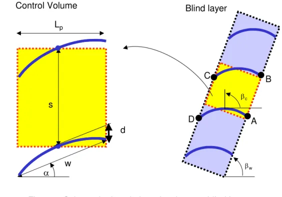
4.5.2 Slat-Type blinds

Figure 5 shows a slat-type blind layer at a tilted window position. The blind slats may be opaque or perforated (with openness factor ϕs). The radiative properties of slats may, thus, be given by the above screen model (equations 21 to 23).

The slats may enclose an open air space, particularly when they are fully open (slat angle α = 0). If the blind layer is subject to a temperature

difference at its front and back environments, a cellular flow may develop in the air space between slats (Machin et al., 1998; Naylor and Lai, 2007). This cavity flow may increase the heat transfer through the blind layer. Further, the environment air may flow though the porous blind layer, but its effect on heat transfer may be neglected due low velocities and relatively high-pressure losses through the blind layer. To account for the effect of the slat cavity flow on heat transfer, the air cavity is assumed as a solid material with an

equivalent thermal conductivity. Temperature gradients through a blind layer denote thus the average of the slat and enclosed air cavity temperatures. Using a representative control volume as shown in Figure 5, the effective thermal properties of a blind layer are calculated as follows:

(

)

sm eq b k k k = 1−ω ⋅ +ω⋅ (25)

(

)

sm a b = −ω ⋅ρ +ω⋅ρ ρ 1 (26)

( ) (

ρc b = 1−ω

) ( )

⋅ ρc sm+ω⋅

( )

ρc a (27)

where:

csm : specific heat of slat material (J/kg.K)

kb : effective thermal conductivity of blind layer (W/mK)

keq : equivalent thermal conductivity of the air cavity between slats (W/mK) ksm : thermal conductivity of slat material (W/mK)

ρsm : density of slat material (kg/m3)

The porosity of a blind layer (ω) is equal to one minus the ratio of the slat material volume to the volume of a representative control volume as shown in Figure 5:

(

s

)

p s s s t s L t L + ⋅ ϕ − − = ω 1 (1 ) (28)

where ϕs, Ls and ts are openness factor, length and thickness of a slat,

respectively. Equation (28) accounts for curved and thick slats, and therefore their effect on the thermal bridging is accounted for in the effective thermal conductivity of blinds.

The equivalent thermal conductivity (keq) of the cavity between slats (denoted by ABCD in Figure 5) may be determined based on the convection film

coefficient of a rectangular cavity subject to temperature differential at its open boundary surfaces (AB and DC) and adiabatic conditions at slat surfaces (BC and AD) as follows:

w z w T T h k_eq = _c( _h− _c, , _c,β_c)⋅ (29) where:

hc : film coefficient of between slats cavity (W/m2K).

Th : temperature of the hot open surface of between slats cavity (K). Tc : temperature of the cold open surface of between slats cavity (K).

w : thickness of between slats cavity (equal to the slat width) (m). zc : height of between slats cavity (m).

βc : inclination angle of between slats cavity (radians).

The height and inclination angle of the between slats cavity are determined as follow: α ⋅ = coss z_c (30) α + β − π = β π > β α + β = β_{c w} , if _c /2; otherwise, _{c w} (31) where: s : spacing of slats (m). α : tilt angle of slats (radians). βw : tilt angle of window (radians).

As for the effective radiative properties of a blind layer, Yahoda and Wright (2004b) presented details on the corresponding calculation procedures.

4.5.3 Drapes

Drapes are similar to screen shadings, except that the drapery fabric may be folded or pleated along the window width, hence forming open vertical

pockets of air. In addition to the characteristics of a screen layer as

mentioned before, drapes are characterized by the fullness factor (Fr), which indicates the ratio of the drapery fabric width to the window width. Fullness factors of 1.5 and 2 are typical values. The enclosed air pocket cavity may affect the heat transfer through the drapery layer if the latter is subject to temperature differential at its boundary environments. Further, the

environment air may flow though the drapery porous layer, but its effect on heat transfer may be neglected due low velocities. Similar to a blind layer, flow within the air pocket cavities may be accounted for by an equivalent thermal conductivity. Equation (29) may, thus, be used for a drapery layer. Approximating the drapery configuration as a sequence of one-sided open rectangular cavity (Kotey et al., 2009a; Farber et al., 1963), as shown in

Figure 6, the cavity characteristics used to calculate the film coefficient in equation (29) are: cavity height (zc) and tilt angle (βc) are equal to the heig and tilt angle of window, and the cavity thickness (w) is equal to the thickness of the drapery layer (Lp) minus the thickness of the drapery material fabric. Note that, the air pocket cavities are finite in the direction of the fenestration width, and, therefore, proper correlations to account for the effect of cavity width (s) should be used to compute the film coefficient in equation (29). W regard to the effective radiative properties of a drapery layer, a proper radiation heat balance over a representative control volume as shown i Figure 6, yields the following relationship:

ht ith n

(

)

(

)

(

)(

)

4 , , , , , , , 3 , , , , , , 1 1 1 1 2 1 2 1 cc f d b d cc f d cc b d cc f d cc cc b d b d cc b d f d cc b d f d f d f eff F F F F F F F F τ τ − ρ − ρ − ρ − + τ ⋅ ε + τ τ + ρ − ε + ε = ε (32)

(

)

(

₍

)

(

)

₎₍

(

)

₎

(

₄

)

, , , , , , 2 , , , , , 1 1 1 1 1 1 2 _{df cc db cc df db cc} cc b d f d cc f d cc f d cc cc b d cc f d f eff F F F F F F F F F τ τ − ρ − ρ − τ + ρ τ + ρ − + + ρ − − ⋅ τ = τ (33) where:

form factor of the pocket cavity surface to itself.

d,b urfaces of a drapery

d,f d,f : long wave effective reflectances of the front and back surfaces

d,f d,b ave effective transmittance of the front and back

tion properties of a drapery sheet are

he cavity Fcc :

εd,f, ε : effective emissivity of the front and back s sheet.

ρ , ρ

of a drapery sheet. τ , τ : long w

surfaces of a drapery sheet. The long-wave effective radia

determined using the previous screen model (equations 21 to 23). T form factor Fcc may be expressed as a function of the fullness factor as follows: 1 2 1 2 − − = Fr Fr F_cc (34)

Figure 7 shows the profiles of

transmittance of drapery layers with an opaque fabric (τm = 0, εm = 0.9) as a

The above models are implemented in the research version of SkyVision perimental measurement

h

6) conducted laboratory measurements to te the e g ss U f ctor of a double glazed window with

x 604

e

the prediction of the numerical model.

the effective emissivity and infrared

function of the openness and the fullness factors.

5 MODEL VALIDATION AND ASSESSMENT

(NRC, 2008), and validated using the available ex

and CFD numerical calculations of centre of glass U-factor of windows wit between-pane and internal Venetian blinds. The following sections provide details on the comparative studies.

5.1 EXPERIMENTAL VALIDATION

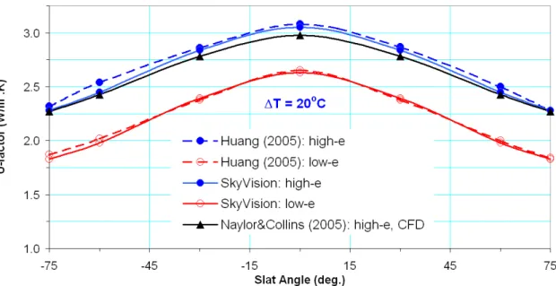
Huang (2005) and Huang et al. (200 compu c ntre of la - a

integrated Venetian blinds using the Guarded Heated Copper Plate apparatus. The plate dimension were 635 mm x 635 mm (or 604 mm

mm without the spacer section). Three sets of window cavity spacing were considered in the measurement: 17.78 mm, 25.4 mm, and 40 mm. The window was made up of 3 mm glass sheets with two high and low emissivity values (0.84 and 0.164 on the hot surface). The blinds were made of

aluminium-alloy slats with the following characteristics: slat thickness = 0.2 mm, slat width w = 14.79 mm, slat spacing s = 11.84 mm, slat curvatur height d =1.5 mm, and slat emissivity of 0.792. To initiate heat flow through the window and blind system, the hot plate was maintained at a temperature of 30oC, and the cold plate took two temperature values of 20oC and 10oC. The heat flux was measured at the hot plate at three locations: centre and edge-end sections, each covering a surface area of 200 mm x 200 mm. The centre of glass U-factor was calculated based on the centre heat flux

measurement and assumed values for the interior and exterior film

coefficients of 8 W/m2K and 23 W/m2K, respectively. The window and blind system and measurement setup were also simulated using a CFD numerical method (Naylor and Collins, 2005; Avedissian and Naylor, 2007) to validate

Figures 8 to 10 show a comparison between the measurement and CFD results and the current model for the three cavity gap spacing values, respectively. The predictions from the current model are in a very good

ar tained

.

er

s U-factor of a double glazed window with internal Venetian simple model, which combines a

one-as s: . d s ). film coefficient of 16.77 W/m K).

agreement with both the measurement and CFD calculations for the regul and low-emissivity windows. Similar comparison results were also ob for other temperature boundary conditions and cavity gap spacing values The maximum difference of about 6% was observed for a window with a low-emissivity coating and large gap spacing (40 mm) when slats are almost closed (Figure 9). The current model provided better results than the simple model of Avedissian and Naylor (2007), which over-estimated the U-factor by about 10%. This simple model combines the one-dimensional heat transf through the window panes, and the CFD-based correlations of the cavity film coefficient.

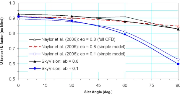
5.2 NUMERICAL VALIDATION

Naylor et al. (2006) employed a full CFD numerical simulation to compute the centre of glas

blinds. Shahid (2003) also proposed a

dimensional heat transfer through the window and blind layers, and CFD-based correlations for the cavity film coefficients. The modelled window w made up of two 3 mm regular glass sheets spaced 12.7 mm apart. The blinds were made of aluminium-alloy slats with the following characteristic slat thermal conductivity = 123 W/mK, slat thickness = 0.16 mm, slat width w = 25.4 mm, slat spacing s = 22.28 mm, and slat curvature height d = 1 mm The blinds were spaced from the window surface so that the slat-tip to glass distance was maintained at 27.5 mm, or 7.7 mm. The CFD calculations as well as the current model assumed that the air cavity between the window an blinds was open at the side, top and bottom sections. The current model use the ISO model for a ventilated gap to compute the gap velocity in equation (1 The performance of the window and blind system was evaluated under the ASHRAE boundary conditions: Indoor temperature = 24oC, outdoor

temperature = 32oC and wind speed = 3.5 m/s (with corresponding outdoor 2