Spatial distribution of the groundwater quality using kriging and Co-kriging interpolations

(1)

See discussions, stats, and author profiles for this publication at: https://www.researchgate.net/publication/343815689

Study of the spatial distribution of groundwater quality index using

geostatistical models

Article in Groundwater for Sustainable Development · August 2020 DOI: 10.1016/j.gsd.2020.100473 CITATIONS 0 READS 85 3 authors:

Some of the authors of this publication are also working on these related projects: Groundwater and surface water qualityView project

Groundwater surface water quality and statistical analysisView project Lazhar Belkhiri

University of Mustafa Ben Boulaid-Batna, Algeria

49PUBLICATIONS 980CITATIONS SEE PROFILE Ammar Tiri Université Batna 2 15PUBLICATIONS 329CITATIONS SEE PROFILE Lotfi Mouni Université de Bouira 66PUBLICATIONS 932CITATIONS SEE PROFILE

All content following this page was uploaded by Lazhar Belkhiri on 14 October 2020. The user has requested enhancement of the downloaded file.

(2)

Groundwater for Sustainable Development 11 (2020) 100473

Available online 22 August 2020

Research paper

Spatial distribution of the groundwater quality using kriging and

Co-kriging interpolations

Lazhar Belkhiri

a,*

_{, Ammar Tiri}

a

_{, Lotfi Mouni}

b

a_{Laboratory of Applied Research in Hydraulics, University of Mustapha Ben Boulaid - Batna 2, Algeria}

b_{Laboratoire de Gestion et Valorisation des Ressources Naturelles et Assurance Qualité, Faculté des Sciences de La Nature et de La Vie et Sciences de La Terre, Université} de Bouira, 10000, Algeria A R T I C L E I N F O Keywords: Groundwater quality Hydrochemical parameters GWQI Kriging Co-kriging methods A B S T R A C T

The present work is aimed for investigation the groundwater quality for drinking purposes in El Mila plain, Algeria. This is carried out through an integrated approach of groundwater quality index (GWQI) and geo-statistical method for mapping this index based on 35 wells and then hydrochemical parameters. Kriging has become a widely used interpolation method to estimate the spatial distribution of the groundwater quality index. The main objective of this study is to evaluate two geostatistical interpolation methods such as Ordinary kriging (OK) and Co-kriging (CK) for enhanced spatial interpolation of the groundwater quality index. The results of GWQI show that about 11.43% of the total samples fall in the excellent water class, and 85.71% samples reported good water quality type, whereas 2.86% groundwater samples exhibited poor water quality type. GWQI had a very strong significant correlation with EC, Ca, Mg, SO4 and HCO3. Therefore, these parameters were used as co-

variables for Co-kriging method. The prediction performance of the adopted interpolation methods is assessed through cross-validation test. The results show that Co-kriging model with electrical conductivity (EC) as co- variable is superior to the other models to predict the groundwater quality index.

1. Introduction

Groundwater is the most important natural resource used for drinking by many people around the world. The variation of the groundwater quality is a function of physical and chemical patterns in an area determined by geological and anthropogenic activities. Since the quality of groundwater resources is as important as its quantity; thus, it is also necessary that the quality of the groundwater resources should be essentially taken into the full consideration (Neisi et al., 2018; Abbasnia et al., 2018). In recent years, with increasing number of physical and chemical parameters of groundwater, a broad scope of geostatistical methods is now utilized for proper analysis and interpretation of infor-mation. More and more researchers are concentrating on the evaluation of the spatial distribution of groundwater quality using many geo-statistical methods in recent decades (Guettaf et al., 2014; Kumar et al., 2014; Singh et al., 2013; Belkhiri and Lotfi, 2014).

Geostatistical method is a useful tool for analyzing the structure of spatial variability, interpolating between point observations and creating the map of interpolated values with an associated error map (Zhou et al., 2011; Arslan, 2012). Several studies have reported that

groundwater quality is generally characterized by a significant spatial variation (Taghizadeh-Mehrjardi, 2014; Alexander et al., 2017; Mar-oufpoor et al., 2017). This suggests that geostatistical methods, which are explicitly able to incorporate the spatial variability of groundwater quality into the estimation process should be employed. Nowadays, different geostatistical techniques methods being widely used for pre-diction of spatial variations of groundwater quality (Nazari Zade et al., 2006; Jasmin and Mallikarjuna, 2014; Belkhiri and Narany, 2015, 2017). Kriging is one of the geostatistical interpolation approaches consist of several methods, including Indicator kriging, Simple kriging, Ordinary kriging and Co-kriging, which commonly applied in estimating spatial distribution of variables (Lee et al., 2007; Babiker et al., 2007; Dindaroglu, 2014; Gyamfi et al., 2016). Ahmadi and Sedghamiz (2007) analyzed the spatial and temporal variations of groundwater level using Ordinary kriging and Co-kriging methods. Delbari (2010) estimated the salinity and the depth of groundwater using Ordinary kriging, Co-kriging, and the inverse fourth power of distance methods. Also, Hooshmand et al. (2011) applied kriging and Co-kriging methods to evaluate the chloride content and sodium adsorption ratio in the groundwater.

* Corresponding author.

E-mail addresses: belkhiri_laz@yahoo.fr, belkhiri.la@gmail.com (L. Belkhiri).

Contents lists available at ScienceDirect

Groundwater for Sustainable Development

journal homepage: http://www.elsevier.com/locate/gsd

https://doi.org/10.1016/j.gsd.2020.100473

(3)

Groundwater for Sustainable Development 11 (2020) 100473

2

The objectives of this study are: (1) to compute the groundwater quality index (GWQI), (2) to determine the relationships between GWQI and hydrochemical parameters in groundwater, and (3) to evaluate and compare the Kriging and the Co-kriging procedures to estimate the groundwater quality index on unobserved points.

2. Study area and data description

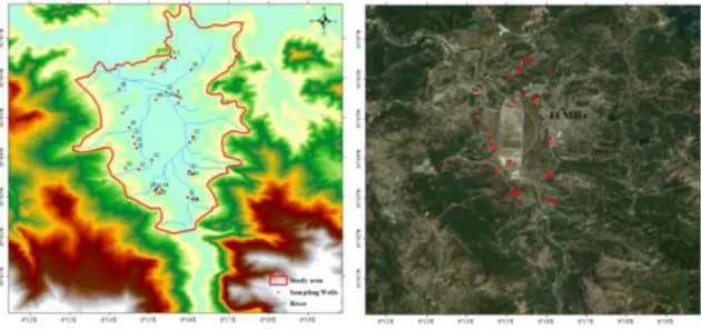
Fig. 1 shows the geographical locations of the study area and groundwater sampling wells. The study area is situated in El Mila plain at a few kilometers from the Mediterranean Sea and between eastern longitude of 60₁₀’_-60₂₀’_{E and northern latitude of 36}0₄₀’_-360₄₇’_{N. The} El Milia region has a Mediterranean climate characterized by warm summers and mild winters but is very humid. The average annual of temperature and precipitation is 17 ◦_{C and 930 mm, respectively (}

Bel-khiri et al., 2018).

Groundwater samples were collected from 35 wells during April 2015, located in the alluvial aquifer (Mio-Plio-Quaternary). Hydro-geologically, this aquifer is considered as an important reservoir and source of water in this region.

3. Methodology

3.1. Hydrochemical parameter analyzed

The hydrochemical parameters used in this study consist of pH, electrical conductivity (EC) and major dissolved ions such as calcium (Ca), magnesium (Mg), sodium (Na), potassium (K), chloride (Cl), sul-fate (SO4), bicarbonate (HCO3), and nitrate (NO3). The samples were collected in April 2015 using standard methods (APHA, 2005; ISO, 1993). pH and EC were measured with a multi-parameter WTW (P3 MultiLine pH/LF-SET). Ca and Mg were estimated titrimetrically using 0.05N–0.01 N EDTA. Na and K were analyzed by flame photometer. HCO3 and Cl by H2SO4 and AgNO3 titration, respectively, and SO4 by turbidimetric method (Clesceri et al., 1998). NO3 was analyzed with UV–visible spectrophotometer. The accuracy of the chemical analysis was verified by calculating ion-balance errors where the errors were generally around 5%. The accuracy of the chemical ion data was calculated using charge balance equation given below, and the charge balance error (CBE) of the groundwater samples was within the accepted limits of ±5%. CBE(%) = ∑ cations − ∑anions ∑ cations +∑anions*100 (1)

Fig. 1. Location of the study are and groundwater samples. Table 1

Relative weight of hydrochemical parameters in study area.

Parameters Si=WHO Standard (2004) Weight (wi) Relative weight (Wi)

pH 8.5 3 0.081 EC 500 5 0.135 Ca 75 5 0.135 Mg 50 4 0.108 Na 200 3 0.081 K 12 2 0.054 Cl 250 5 0.135 SO4 250 3 0.081 HCO3 500 5 0.135 NO3 45 2 0.054 Sum 37 1.000 Table 2

Classification of groundwater based on GWQI (Sahu and Sikdar, 2008).

Range Type of water Numbers of wells

<50 Excellent water 4

50–100.1 Good water 30

100–200.1 Poor water 1

200–300.1 Very poor water 0

>300 Water unsuitable for drinking purposes 0

Table 3

Statistical descriptive of the hydrochemical parameters and GWQI.

Parameters Min Max Mean Std.

dev Coef. var Numbers of wells exceeding the standard pH 6 7.5 6.77 0.26 4 0 EC 228 1411 821 279 34 30 Ca 16 198 96 32 34 28 Mg 11.02 61.32 37.39 12.01 32.12 5 Na 12.47 38.14 24.57 4.99 20.29 0 K 1.78 5.45 3.51 0.71 20.29 0 Cl 63.90 255.60 150.08 53.12 35.40 1 SO4 61.39 270.00 125.97 49.93 39.64 2 HCO3 97.60 524.60 232.02 90.22 38.88 1 NO3 0.02 47.54 23.47 14.77 62.90 2 GQWI 44.55 102.49 70.11 15.05 21

Min: Minimum; Max: Maximum; Std.dev: Standard deviation; Coef.var: Coeffi-cient of variation.

(4)

where ∑cations and ∑anions are the sum of cations and anions, respectively, expressed in equivalents par liter.

3.2. Groundwater quality index (GWQI)

Groundwater quality index (GWQI) method reflects the influence of the hydrochemical parameters of groundwater on the suitability for drinking purposes (Sahu and Sikdar, 2008; Belkhiri et al., 2018). The estimation of the GWQI index was based on parameter weighting. In the current study, three steps were followed in to order to calculate GWQI based on 10 parameters at each well.

In the first step, the relative weight (Wi) of each parameter was estimated as follows: Wi= wi ∑n i=1 wi (2) where wi is the weight of each parameter, and n is the number of pa-rameters. Assigning of weight (wi) to the different groundwater pa-rameters according to their relative importance in the overall quality of groundwater for drinking purposes (weight ranged from 1 to 5). The weights according to the World Health Organization standards (WHO, 2004) are presented in Table 1.

In the second step, the quality rating scale (qi), which related the value of the parameter to the WHO standards, was calculated as follows: qi= ( Ci− Ci0 Si− Ci0 ) *100 (3)

where Ci is the concentrations of each parameter (mg/l), Si is the stan-dard permissible value of each parameter (mg/l). For all parameters, and Ci0 is the ideal value of each parameter in pure water (consider Table 4

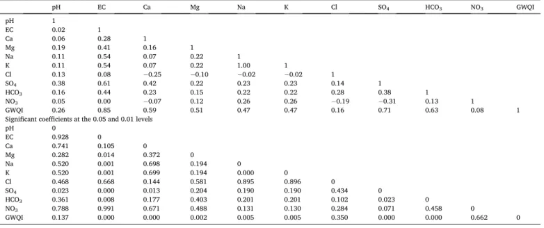
Correlation coefficient matrix of hydrochemical parameters.

pH EC Ca Mg Na K Cl SO4 HCO3 NO3 GWQI

pH 1 EC 0.02 1 Ca 0.06 0.28 1 Mg 0.19 0.41 0.16 1 Na 0.11 0.54 0.07 0.22 1 K 0.11 0.54 0.07 0.22 1.00 1 Cl 0.13 0.08 −0.25 −0.10 −0.02 − 0.02 1 SO4 0.38 0.61 0.42 0.22 0.23 0.23 0.14 1 HCO3 0.16 0.44 0.23 0.15 0.22 0.22 0.28 0.38 1 NO3 0.05 0.00 −0.07 0.12 0.26 0.26 −0.19 −0.31 0.13 1 GWQI 0.26 0.85 0.59 0.51 0.47 0.47 0.16 0.71 0.63 0.08 1

Significant coefficients at the 0.05 and 0.01 levels pH 0 EC 0.928 0 Ca 0.741 0.105 0 Mg 0.282 0.014 0.372 0 Na 0.520 0.001 0.698 0.194 0 K 0.520 0.001 0.699 0.194 0.000 0 Cl 0.468 0.668 0.144 0.581 0.895 0.896 0 SO4 0.023 0.000 0.013 0.204 0.190 0.190 0.434 0 HCO3 0.361 0.008 0.177 0.403 0.201 0.201 0.102 0.023 0 NO3 0.788 0.991 0.671 0.488 0.131 0.130 0.284 0.071 0.458 0 GWQI 0.137 0.000 0.000 0.002 0.005 0.005 0.350 0.000 0.000 0.662 0

Fig. 2. Plot of training (blue color) and testing (red color) data. (For inter-pretation of the references to color in this figure legend, the reader is referred to the Web version of this article.)

Table 5

Best fitted semivariogram models and model parameters for GWQI.

Models Range Nugget (C0) p-sill (C) Nugget-sill ratio ((C0/C0+C)*100) SSErr R2

Exponential 434.6967 0.001951 0.009784 16.63 3.25E-11 0.977175 Spherical 1344.937 0.004263 0.007399 36.55 1.57E-11 0.990538 Gaussian 421.247 0.000802 0.010959 6.82 3.28E-11 0.982465 Linear 1373.8412 0.005699 0.00609 48.34 1.72E-11 0.990209 Matern 434.6967 0.001951 0.009784 16.63 3.25E-11 0.977175 L. Belkhiri et al.

(5)

4 Ci0 =0 for all parameters) except the pH value where C_i0=7).

In the final step, GWQI of each well was given as follows:

GWQI =∑

n

i=1

Wi*qi (4)

The groundwater quality based on GWQI can be classified into five classes, as listed in Table 2.

3.3. Geostatistical methods

Kriging and Co-kriging analysis were performed to produce predic-tion maps of the groundwater quality index (GWQI). Kriging is a geo-statistical technique that is used to interpolate a surface from a scattered set of known points in which a continuous surface of values can be predicted between the known locations. Variogram model controls Kriging weights. Variogram is mathematically defined as a measure of semi-variance as a function of distance.

γ(h) = 1

2N(h) ∑N(h)

i=1

[z(xi) − z(xi+h)]2 (5)

where γ(h) is the semi-variance; N(h) the number of pairs separated by distance or lag h; Z(xi) the measured sample at point xi; and Z(xi +h) the measured sample at point (xi +h). The spatial structure of the data is determined by fitting a mathematical model to the experimental. The mathematical models provide information about the structure of the spatial variation, as well as the input parameters for kriging. The model was fitted to the environmental variables, which showed that these variables had a spatial autocorrelation in their effective ranges. Expo-nential, spherical, Gaussian and Linear models were used to fit the experimental variogram of data pairs.

3.3.1. Ordinary kriging (OK)

OK is a geostatistical interpolation method based on spatially dependent variance, which used to find the best linear unbiased estimate

(Goovaerts, 1997). The general form of Ordinary kriging equation can be written as: ̂ Z(xp ) = ∑n i=1 λiZ(xi) (6)

In order to achieve unbiased estimations in kriging the following set of equations should be solved simultaneously:

∑n i=1 λiγ ( xi,xj ) − μ=γ(xi,xp ) where j = 1, ..., n with ∑n i=1 λi=1 (7)

where ̂Z(xp)is the estimated value of variable Z (i.e., GWQI) at location xp; Z(xi) is the known value at location xi; λi is the weight associated with the data; μ is the Lagrange coefficient; γ(xi,xj) is the value of variogram

corresponding to a vector with origin in xi and extremity in xj; and n is the number of sampling points used in estimation.

3.3.2. Co-kriging method (CK)

CK estimator is the multivariate equivalent to kriging, which has secondary variables. By using multiple datasets, it is a very flexible interpolation method, allowing the user to investigate graphs of cross- correlation and autocorrelation. Co-Kriging estimation is introduced by the following equation:

∑v l=1 ∑n i=1 λilλlvγ ( xi,xj ) − μv=γuv ( xi,xp ) where j = 1, ..., n and u = 1, ..., v with∑ nl i=1 λil= { 1, 1 = u 0, 1 ∕=1u (8) where u and v are the primary and covariate (secondary) variables, respectively. The two variates u and v are cross-correlated and the co-variate contributes to the estimation of the primary co-variate.

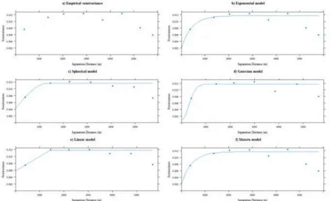
Fig. 3. a) Empirical semivariance of GWQI and its fitted model: b) Exponential model, c) Spherical model, d) Gaussian model, e) Linear model and f) Matren model. L. Belkhiri et al.

(6)

For CK analysis, the cross-variogram should be determined in prior. The cross-variogram models between the primary and secondary vari-ables are obtained by fitting with an experimental cross-variogram that is given by γuv(h) = 1 2N(h) ∑N(h) i=1 [zu(xi) − zu(xi+h)][zv(xi) − zv(xi+h)] (9)

Ordinary kriging (OK) and Co-kriging (OK) analysis were performed to produce prediction maps of the groundwater quality index (GWQI) values. The different covariates used in this study are determined based on the significant correlation between groundwater quality index and the different hydrochemical parameters.

3.3.3. Cross-validation method

To evaluate the performance of interpolation methods is used the cross-validation method. In this study, estimated and observed values were compared using mean errors (bias: ME), root mean square errors (precision: RMSE) and squared deviation ratio (MSDR). The smallest ME, RMSE and MSDR indicate the most accurate predictions.

Some R packages are designed delicately for kriging, in this study, we use “gstat”, “rgdal”, “maptools”, “sp”, “lattice” packages to implement a common type of spatial interpolation.

4. Results and discussions

4.1. Statistical descriptive of the hydrochemical parameters

A statistical summary of hydrochemical data of groundwater samples is given in Table 3. All the groundwater samples showed the pH values ranged from 6 to 7.5 with a mean value of 6.77, indicating acidic to slight alkaline in nature. The electrical conductivity values of the sam-ples ranged from 228 to 1411 μS/cm with a mean of 821 μS/cm which

presents the high amount of salts in the groundwater. Most of the groundwater samples (86%) showed high value of EC and may not be suitable for drinking purposes (WHO, 2004). The calcium and magne-sium values of the samples ranged from 16 to 198 and 11.02–61.32 mg/l mg/l with a mean of 96 and 37.39 mg/l respectively. The results revealed that, 80% and 14% of total samples for Ca and Mg, respectively, were above the limits fixed by WHO (2004). High con-centration of Ca and Mg in groundwater could cause some negative ef-fects like health effect such as abdominal ailments as well as economic and hydraulic effect such as scaling. The values of sodium and potassium varied from 12.47 to 38.14 mg/l and 1.78–5.45 mg/l, respectively, indicating that all values for both cations were lower than the WHO standard level (WHO, 2004). Cl concentration in the area varied from 63.9 to 255.6 mg/l with a mean of 150.08 mg/l. SO4 values in the area ranged from 61.39 to 270 mg/l with mean value 125.97 mg/l. Bicar-bonate concentration in groundwater ranged from 97.60 to 524.6 with a

Fig. 4. Spatial prediction map of GWQI (log10) obtained by a) Ordinary Kriging (OK), b) Co-Kriging (CK) with EC, c) CK with Ca, d) CK with Mg, e) CK with SO4 and

f) CK with HCO3. Black dots are groundwater samples.

(7)

6 mean of 232.02 mg/l. Only one sample for chloride and bicarbonate and two samples for sulfate were lower than the WHO standard level (WHO, 2004), while the other samples were within the WHO standard for drinking water. Nitrate and nitrite concentration were found in samples ranged from 0.02 to 47.54 mg/l and 0.01–47.54 mg/l, respectively. Two samples were found to be exceeding the WHO for NO3.

Understanding the relationship and variations between the different hydrochemical parameters and explaining the interaction between them could be carried out based on the statistical analysis (Meireles et al., 2010; Ahamad et al., 2018). The contamination of groundwater is pri-marily accountable for the variations in electrical conductivity. The relationship between different parameters is shown in Table 4. Ac-cording to the results, pH-SO4 (0.38), Ca–SO4 (0.42), Na–K (1.00), and SO4–HCO3 (0.38) indicate significant correlations. Significant positive correlation between EC and Mg (0.41), Na–K (0.54), SO4 (0.61), and

HCO3 (0.44) is suggestive of significant natural and anthropogenic ac-tivities leading to the addition of these ions into the groundwater of the region.

4.2. Evaluation of drinking water quality

Suitability of groundwater quality for drinking water purposes could be distinguished based on the hydrochemical parameters. Rating of groundwater in the aspect of quality and consumption using the influ-ence of individual water quality parameters can be helpful in making decision by managers and administrative organizations.

The results of GWQI of the groundwater samples are presented in

Tables 2 and 3 The GWQI values ranged from 44.55 to 102.49 with a

mean value of 70.11, which can be placed in three classes, namely poor water, good water, and excellent water quality. The results revealed that

Fig. 5. Spatial prediction errors map of GWQI (log10) obtained by a) Ordinary Kriging (OK), b) Co-Kriging (CK) with EC, c) CK with Ca, d) CK with Mg, e) CK with

SO4 and f) CK with HCO3. Black dots are groundwater samples.

Table 6

Compare the cross-evaluation errors for different models.

Models Min Mean Max ME RMSE MSDR

OK −0.1816 −0.00235 0.171359 −0.00235 0.100787 1.163582 CK with EC −0.15326 0.001778 0.115835 0.001778 0.051449 0.747344 CK with Ca −0.2334 −0.00469 0.390785 −0.00469 0.116067 8.181616 CK with Mg −0.24811 0.00435 0.217444 0.00435 0.098116 2.615486 CK with SO4 −0.17292 −0.00028 0.153277 −0.00028 0.080772 4.094798 CK with HCO3 −0.24523 −0.00325 0.13982 −0.00325 0.094937 4.930154 L. Belkhiri et al.

(8)

about 11.43% of the groundwater samples fall in the excellent water class, and 85.71% samples reported good water quality type, whereas 2.86% groundwater samples exhibited poor water quality type. Form Table 4, we can see that GWQI had a significant positive correlation with EC (0.85), SO4 (0.71), HCO3 (0.63), Ca (0.59), Mg (0.51), and Na–K (0.47). The strong significant correlation of the parameters such as EC, Ca, Mg, SO4 and HCO3 with GWQI is selected as co-variables to pre-dicted spatially the groundwater quality index. In this study, we compared five possible co-variables based on their strong significant correlation with GWQI.

4.3. Spatial interpolation method

The groundwater quality index (GWQI was interpolated by Kriging and Co-kriging (CK) methods. The data frame of water sample points contains 35 wells (observations) and the prediction grid has 15088 lo-cations, spaced every 50 m in both the East and North grid directions, covering the irregularly-shaped study area. Because of the wide nu-merical range of the GWQI values we worked with the log-transformed target variable; to allow easy interpretation of the results we used base- 10 logarithms (log10) for each parameter. In order to experiment an independent validation, we first need to separate the data into a training data and test data. Then we use the training dataset to predict the value in the test dataset. In this study, 30% of the data has been excluded for testing (Fig. 2).

4.3.1. Selecting the best fitted variogram models

The spatial dependence of the groundwater quality index was determined by semivariance analysis, which indicated that the calcu-lated index was modeled with different semivariogram models with a nugget effect. Sum of squares errors (SSErr) and regression coefficient

(R2_{) provided an exact measure of how well the model fit the variogram} data, with lower SSErr and higher R2 _{indicating better model fits. The} parameter values of the different fitted models are presented in Table 5. Theory and empirical semivariogram were prepared for the GWQI as shown in Fig. 3. The results of the selecting of the best fitted variogram model show that spherical model was found as the most accurate model for GWQI.

Spatial dependency is commonly accessed in terms of the ratio of nugget (C0) to sill (C0+C) expressed in percentage. In this respect, the GWQI index is considered as a strong spatial dependence when the value of ratio is less than 25%, a moderate spatial dependence when this value is between 25% and 75%, and a weak spatial dependence when the value is greater than 75%. Form Table 5, we see clearly that the spatial dependence of GWIQ for the best fitted semivariogram model is mod-erate with a ratio of 36.55%.

4.3.2. Ordinary Kriging and Co-Kriging interpolations of the GWQI The best fitted model (spherical model) of regionalization is used to interpolate the groundwater quality index (log10 GWQI) with both Or-dinary kriging (OK) and Co-kriging (CK) methods on the prediction grid. First, we predict the GWQI without the co-variables. Then, CK method is applied with EC, Ca, Mg, SO4, and HCO3 as co-variables to predicted the groundwater quality index.

In this step, we compare graphically the predictions and their errors of the GWQI variable form OK and CK. Figs. 4 and 5 show the predictions and their errors of the GWQI (log10) distribution across the study area from different models. The maps of CK with co-variables provide some new regions where the GWQI values are high. The high values of GWQI could be observed in the center of the plain near to the El Milia city and southern region, which might be principally caused by both anthropo-genic activities and erosion of natural deposits.

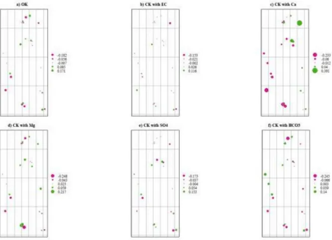
Fig. 6. Spatial distribution of the evaluation errors for: a) Ordinary Kriging (OK), b) Co-Kriging (CK) with EC, c) CK with Ca, d) CK with Mg, e) CK with SO4 and f) CK

with HCO3.

(9)

8 From Fig. 5, we can see that the OK prediction errors map shows the expected low errors near the water sample points, whereas CK with different co-variables gives the lowest errors averaged across the map. This is because the co-kriging predictions are based not only on the target variable (GWQI) but also the co-variable at these points as well as their covariance (Rossiter, 2018).

4.3.3. Evaluation of geostatistical methods

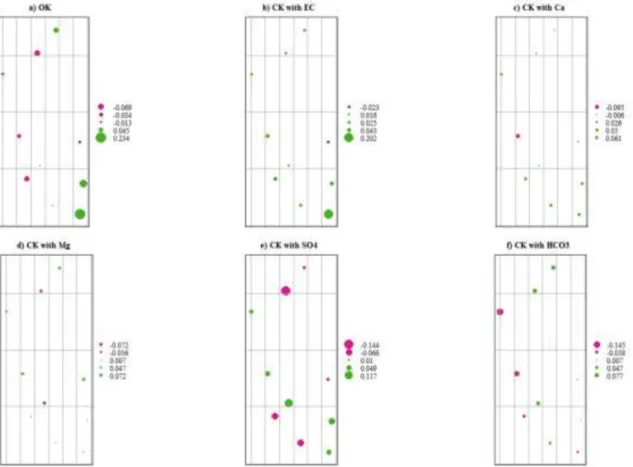
For the evaluation, we used the cross-validation performance to evaluate the performance of the different interpolations based on the testing dataset (30%). To compare the evaluations for the different models, diagnostic measures such as ME (mean errors), RMSE (root mean square errors) and MSDR (squared deviation ratio) of the residuals to the prediction errors are calculated (Table 6). Fig. 6 shows bubble plots of the cross-evaluation errors for all models where positive values are plotted in green blue and negative in red, with the size of the bubble proportional to the distance from zero. From Table 6 and Fig. 7, we see clearly that the Co-kriging model with EC as co-variable is superior to the other models in all measures.

5. Conclusion

In this study, geostatistical interpolation methods were used in order to understand the spatial distribution of the groundwater quality index (GWQI). Descriptive and correlation analysis were conducted to deter-mine the significant correlations between GWQI and all parameters. Strong significant correlation was observed between GWQI and EC, Ca, Mg, SO4 and HCO3, indicating the significant natural and anthropogenic activities leading to the addition of these ions into the groundwater. Ordinary Kriging and Co-kriging procedures were applied to estimate the spatial distribution of GWQI values at the unobserved locations of

the study area. For CK method, EC, Ca, Mg, SO4 and HCO3 were considered as co-variables. Cross-validation was estimated to evaluate and compare the performance of the different proposed models. The results show that Co-kriging with electrical conductivity as co-variable is higher than the other models which means its higher accuracy than Kriging method to predict the groundwater quality index.

Declaration of competing interest

The authors declare that they have no known competing financial interests or personal relationships that could have appeared to influence the work reported in this paper.

Acknowledgements

The authors thank the editor Prof. Prosun Bhattacharya and anony-mous reviewers for their comments which greatly improved this manuscript.

Appendix A. Supplementary data

Supplementary data to this article can be found online at https://doi. org/10.1016/j.gsd.2020.100473.

References

Abbasnia, A., Yousefi, N., Mahvi, A.H., Nabizadeh, R., Radfard, M., Yousefi, M., Alimohammad, M., 2018. Evaluation of groundwater quality using water quality index and its suitability for assessing water for drinking and irrigation purposes: case study of Sistan and Baluchistan province (Iran). Human and Ecological Risk Assessment 2 (2). https://doi.org/10.1080/10807039.2018.1458596.

Fig. 7. Spatial distribution of the cross-evaluation errors for: a) Ordinary Kriging (OK), b) Co-Kriging (CK) with EC, c) CK with Ca, d) CK with Mg, e) CK with SO4 and

f) CK with HCO3.

(10)

9

Ahmadi, S.H., Sedghamiz, A., 2007. Geostatistical analysis of spatial and temporal

variations of groundwater level. Environ. Monit. Assess. 129 (1–3), 277–294.

Ahamad, A., Madhav, S., Singh, P., Pandey, J., Khan, A.H., 2018. Assessment, of groundwater quality with special emphasis on nitrate contamination in parts of

Varanasi City, Uttar Pradesh, India. Applied Water Science 8, 115.

Alexander, A.C., Ndambuki, J., Salim, R., Manda, A., 2017. Assessment of spatial variation of groundwater quality in a mining basin. Sustainability 9, 823. https://

doi.org/10.3390/su9050823.

American Public Health Association (APHA), 2005. Standard Methods for the Examinations of Waters and Waste Waters 21st. APHA AWWA-WEF, Washington,

DC.

Arslan, H., 2012. Spatial and temporal mapping of groundwater salinity using ordinary kriging and indicator kriging: the case of Bafra Plain. Turkey. Agric. Water Manag.

113, 57–63.

Babiker, I.S., Mohamed, M.A., Hiyama, T., 2007. Assessing groundwater quality using GIS. Water Resour. Manag. 21, 699–715. https://doi.org/10.1007/s11269-006-

9059-6.

Belkhiri, L., Lotfi, M., 2014. Geochemical characterization of surface water and

groundwater in soummam basin, Algeria. Nat. Resour. Res. 23 (4).

Belkhiri, L., Narany, T.S., 2015. Using multivariate statistical analysis, geostatistical techniques and structural equation modeling to identify spatial variability of

groundwater quality. Water Resour. Manag. 29 (6), 2073–2089.

Belkhiri, L., Mouni, L., Narany, T.S., Tiri, A., 2017. Evaluation of potential health risk of heavy metals in groundwater using the integration of indicator kriging and multivariate statistical methods. Groundwater for Sustainable Development 4,

12–22.

Belkhiri, L., Mouni, L., Tiri, A., Narany, T.S., Nouibet, R., 2018. Spatial analysis of groundwater quality using self-organizing maps. Groundwater for Sustainable

Development 7, 121–132.

Clesceri, L.S., Greenberg, A.E., Eaton, A.D., 1998. Standard Methods for the Examination of Water and Wastewater, twentieth ed. American Public Health Association,

American Water Works Association, Water Environment Federation, Washington.

Delbari, M., Miremadisar, Afrasiab pour, 2010. The analysis of the spatial and time changes in salinity and depth of groundwater (Case study: mazandaran province). J.

Irrigat. Drain. Iran 3 (4), 359–374.

Dindaroglu, T., 2014. The use of the GIS Kriging technique to determine the spatial changes of natural radionuclide concentrations in soil and forest cover. J. Environ. Health Sci. Eng. 12, 130. https://doi.org/10.1186/s40201-014-0130-6.

Goovaerts, P., 1997. Geostatistics for Natural Resources Evaluation. Oxford University

Press, New York.

Guettaf, M., Maoui, A., Ihdene, Z., 2014. Assessment of water quality: a case study of the seybouse river (North East of Algeria). Appl Water Sci. https://doi.org/10.1007/

s13201-014-0245-z.

Gyamfi, C., Ndambuki, J., Diabene, P., Kifanyi, G., Githuku, C., Alexander, A., 2016. Using GIS for spatial exploratory analysis of borehole data: a firsthand approach towards groundwater development. J. Sci. Technol. 36, 38–48. https://doi.org/

10.4314/just.v36i1.7.

Hooshmand, A., Delghandi, M., Izadi, A., Aali, K.A., 2011. Application of kriging and cokriging in spatial estimation of groundwater quality parameters. Afr. J. Agric. Res.

14 (6), 3402–3408.

International Standards Organization (ISO), 1993. Water Quality Sampling Part 11:

Guidance on Sampling of Ground Waters. ISO5667-11.

Jasmin, I., Mallikarjuna, P., 2014. Physicochemical quality evaluation of groundwater and development of drinking water quality index for Araniar River Basin, Tamil

Nadu, India. Environ. Monit. Assess. 186, 935–948.

Kumar, V.S., Amarender, B., Dhakate, R., Sankaran, S., Kumar, K.R., 2014. Assessment of groundwater quality for drinking and irrigation use in shallow hard rock aquifer of Pudunagaram, Palakkad District Kerala. Appl Water Sci. https://doi.org/10.1007/

s13201-014-0214-6.

Lee, J.J., Jang, C.S., Wang, S.W., Liu, C.W., 2007. Evaluation of potential health risk of arsenic-affected groundwater using indicator kriging and dose response model. Sci.

Total Environ. 384 (1), 151–162.

Maroufpoor, S., Fakheri-Fard, A., Shiri, J., 2017. Study of the spatial distribution of groundwater quality using soft computing and geostatistical models. ISH Journal of Hydraulic Engineering 25 (2), 232–238. https://doi.org/10.1080/

09715010.2017.1408036.

Meireles, A., Andrade, E.M., Chaves, L., Frischkorn, H., Crisostomo, L.A., 2010. Anew

proposal of the classification of irrigation water. Rev. Cienc. Agron. 41 (3), 349–357.

Nazari Zade, F., Arshadiyan, F., Zand-Vakily, K., 2006. Study of Spatial Variability of Groundwater Quality of Balarood Plain in Khuzestan Province. The First Congress of Optimized Exploitation from Water Source of Karoon and Zayanderood Plain. Shahre

kord University, pp. 1236–1240.

Neisi, A., Mirzabeygi, M., Zeyduni, G., 2018. Data on fluoride concentration levels in cold and warm season in City area of Sistan and Baluchistan Province, Iran. Data Brief 18, 713–718. https://doi.org/10.1016/j.dib.2018.03.060.

Sahu, P., Sikdar, P.K., 2008. Hydrochemical framework of the aquifer in and around East

Kolkata Wetlands, West Bengal, India. Environ. Geol. 55, 823–835.

Singh, P.K., Tiwari, A.K., Panigarhy, B.P., Mahato, M.K., 2013. Water quality indices used for water resources vulnerability assessment using GIS technique: a review. Int.

J. Earth Sci. Eng. 6 (6–1), 1594–1600.

Taghizadeh-Mehrjardi, R., 2014. Mapping the spatial variability of groundwater quality

in urmia, Iran. J. Mater. Environ. Sci. 5 (2), 530–539.

WHO (World Health Organization), 2004. Guidelines for Drinking-Water Quality, third

ed. World Health Organization (WHO), Geneva.

Zhou, Z.M., Zhang, G.H., Wang, J.Z., Yan, M.J., 2011. Risk assessment of soil salinity by multiple-variable indicator kriging in the low plain around the Bohai Sea. Shuili

Xuebao 42 (10), 1144–1151.