Publisher’s version / Version de l'éditeur:
Proceedings of New Frontiers in Mining Complex Patterns (NFMCP 2012), pp.
12-23, 2012-09
READ THESE TERMS AND CONDITIONS CAREFULLY BEFORE USING THIS WEBSITE. https://nrc-publications.canada.ca/eng/copyright
Vous avez des questions? Nous pouvons vous aider. Pour communiquer directement avec un auteur, consultez la première page de la revue dans laquelle son article a été publié afin de trouver ses coordonnées. Si vous n’arrivez pas à les repérer, communiquez avec nous à [email protected].
Questions? Contact the NRC Publications Archive team at
[email protected]. If you wish to email the authors directly, please see the first page of the publication for their contact information.
NRC Publications Archive
Archives des publications du CNRC
This publication could be one of several versions: author’s original, accepted manuscript or the publisher’s version. / La version de cette publication peut être l’une des suivantes : la version prépublication de l’auteur, la version acceptée du manuscrit ou la version de l’éditeur.
Access and use of this website and the material on it are subject to the Terms and Conditions set forth at
Learning with aggregation and correlation in the presence of large
fluctuations
Paquet, Eric; Viktor, Herna L.; Guo, Hongyu
https://publications-cnrc.canada.ca/fra/droits
L’accès à ce site Web et l’utilisation de son contenu sont assujettis aux conditions présentées dans le site LISEZ CES CONDITIONS ATTENTIVEMENT AVANT D’UTILISER CE SITE WEB.
NRC Publications Record / Notice d'Archives des publications de CNRC:
https://nrc-publications.canada.ca/eng/view/object/?id=b9860f27-54db-41a7-a16f-662aab2c6528 https://publications-cnrc.canada.ca/fra/voir/objet/?id=b9860f27-54db-41a7-a16f-662aab2c6528Learning with Aggregation and Correlation in the
Presence of Large Fluctuations
Eric Paquet1,2, Herna L. Viktor2, and Hongyu Guo1
1 National Research Council, 1200 Montreal Road, Ottawa, Ontario, K1A 0R6, Canada 2 School of Information Technology and Engineering, University of Ottawa, 800 King
Edward, Ottawa, Ontario, K1N 6N5, Canada
[email protected], [email protected], [email protected]
Abstract. Consider a scenario where one aims to learn models from dynamic and evolving data being characterized by very large fluctuations that are neither attributable to noise nor outliers. This may be the case, for instance, when predicting the potential future damages of earthquakes or oil spills, or when conducting financial data analysis. If follows that, in such a situation, the standard central limit theorem does not apply, since the associated Gaussian distribution exponentially suppresses large fluctuations. In this paper, we present an analysis of data aggregation and correlation in such scenarios. To this end, we introduce the Lévy, or stable, distribution which is a generalization of the Gaussian distribution. Our theoretical conclusions are illustrated with various simulations, as well as against a benchmarking financial database. We show which specific strategies should be adopted for aggregation, depending on the stability exponent of the Lévy distribution. Our results firstly show scenarios where it may be impossible to determine the mean and the standard deviation of an aggregate. Secondly, we discuss the case where an aggregate may have to be characterized with its largest fluctuations. Thirdly, we illustrate that the correlation in between two attributes may be underestimated if a Gaussian distribution is erroneously assumed.
Keywords: Aggregation in Relational Learning, Correlation-based Analysis and Covariance, Lévy Distribution, Stable Distribution.
1 Introduction
Aggregation is an important step when pre-processing data, prior to building a data mining model. This step is crucial when considering complex data that represents interactions between several potentially heterogeneous entities. For instance, in social network analysis the frequency of a particular relationship is often represented by an aggregation based on the number of occurrences. The same observation holds in multi-relational database mining and in spatial data exploration, where aggregation is needed to link multiple tables together [1, 2]. Similarly, data obtained from data streams are frequently summarized into manageable sized buckets or windows, prior to mining.
Often, during a data mining exercise, it is implicitly assumed that large-scale data fluctuations must be either associated with noise or with outliers, or that a concept drift has occurred. The most striking consequence of such an assumption is that, once the noisy data and the outliers have been eliminated, the remaining data may be characterized in two ways. That is, firstly, their typical behaviour (i.e. their mean) and secondly, by the characteristic scale of their variations (i.e. their variance). Fluctuation above the characteristic scale is thus being assumed to be highly unlikely, or assumed to indicate that a model has become outdated. However, there are many categories of data which are characterized by large-scale fluctuations. For instance, surprisingly, supermarket ketchup sales have been shown to be typified by such large-scale fluctuations [4]. Further, financial data and earthquake-related data are also examples of data exhibiting this behaviour [3]. This issue is highly relevant when aiming to build models that predict the potential damages caused by catastrophic events, such as financial market turbulences and tsunamis. The large-scale fluctuations do not origin from noise or outliers, but constitute an intrinsic and distinctive feature of the data. Mathematically speaking, small fluctuations are modelled with the central limit theorem and the Gaussian distribution, while large fluctuations are modelled with the generalized central limit theorem and the Lévy distribution. This paper studies the aggregation of data presenting large-scale fluctuations, to determine their properties, the best approaches for their aggregation and the impact of such behaviour on their correlation.
Our main contributions are as follows. Firstly, we provide a theoretical analysis which shows the importance of taking the data distribution characteristics, when learning involves aggregation and correlation, into account. Secondly, we introduce the stable distribution as a mechanism to allow machine learning methods to compute meaningful aggregated information and to correctly evaluate the correlation when learning from data presenting large fluctuations. Thirdly, we demonstrate the proposed method’s applicability in typical machine learning and data mining problems. Here, we discuss the analysis of financial data and relational learning involving aggregation. We also mention, in Section 4, that our approach is highly relevant for correlation-based privacy preservation data mining.
This paper is organized as follows. In Section 2, we review the fundamental assumptions behind aggregation, namely the central limit theorem and the Gaussian distribution. In Section 3, we introduce a more general distribution for the aggregate, the Lévy or stable distribution, for which the Gaussian distribution is a particular case. We explain how this distribution may be estimated from the empirical data and present some useful properties of the Lévy distribution. Then, we study the rank ordering statistics of the Lévy distribution in order to determine if there are some dominant terms in the distribution. We introduce the multivariate stable distribution in order to generalize, in Section 4, the concepts of covariance and correlation to stable distributions. In Section 5, we present various simulations in order to illustrate the theoretical results obtained in the previous sections, as well as their consequences for aggregation. We show that our methodology is applicable to real world financial data. The last section present our conclusions and directions for future work.
2 Aggregation, Central Limit Theorem and Gaussian Distribution
In this section, we review the basic assumptions on which aggregation is based. Despite the fact that these assumptions are quite general, they do not cover all possible data distributions, for instance, the Lévy distribution. Importantly, as will be shown in Section 5, data associated with catastrophic events such as oil spill, stock market crashes and earthquakes often follows the Lévy distribution and need special care during data pre-processing and model building. Consequently, we aim to understand their strengths as well as their limitations in order to be able to address them in the following sections. Aggregation is based on the standard central limit theorem which may be stated as follow: The sum of N normalized independent and identically distributed random variables of zero mean and finite variance s2 is a random variable with a probability distribution function converging to the Gaussian distribution with variance s2. That means that aggregation, in the sense of a sum of real numbers, has a Gaussian distribution irrespectively of the original distribution of its individual data. This is a very powerful theorem because the Gaussian distribution may be characterized with solely two numbers: its mean m and its variance s2 which are the first two moments of the distribution. In practice, this implies that an aggregation, such as a sum, may be fully characterized by its mean and its variance; this is why aggregation is so powerful. All the other moments of the Gaussian distribution are equal to zero. In the next section, we consider a generalization of the central limit theorem which requires the introduction of the Lévy or stable distribution.
3 Aggregation with an Underlying Lévy Distribution or Stable
Distribution
In this section, we review the Lévy distribution, we show how it may be estimated from the underlying empirical data and we analyze its properties. Finally, we introduce the multivariate Lévy distribution in order to extend the notions of covariance and correlation to data distributed according to a stable distribution. One may associate to a probability distribution L x its Fourier transform or characteristic
( )
function L k . Stable or Lévy distributions are distributions for which the individual
( )
data as well as their sum are identically distributed [5]. This fact implies that the convolution of the individual data is equal to the distribution of the sum or, equivalently, that the characteristic function of the sum is equal to the product of their individual characteristic functions. The Lévy distribution does not have a closed form and is more easily defined from its characteristic function:
( )
(
(
)
)
( ) (
)
(
)
, , , exp exp 1 sgn , L k ik X i k k i k W k a m b g a a m g b a = = - --é
ù
ê
ú
ë
û
E (1) where E( )
is the expectation and where(
,)
tan 2 1 2 ln 1 W k k pa a a a p ìïï ¹ ïïï íï ï- = ïïïî (2)The Lévy distribution is characterized by four parameters as opposed to the Gaussian distribution which is characterized by only two. The parameters are the stability exponent a, the scale parameter g, the asymmetry parameter b and the localisation parameter m . While the tail of the Gaussian distribution is exponentially suppressed, the tail of the Lévy distribution decays as a power law (heavy tail) which depends on its stability exponent a :
( )
1 x C L x x a +a ¥ (3)Eq. (3) shows that extreme values are much more likely for the Lévy distribution that they are for the Gaussian distribution. The reason being that the Gaussian distribution fluctuates around its mean, the scale of the fluctuations being characterized by its variance (the fluctuations are exponentially suppressed) while the Lévy distribution may produce fluctuations far beyond the scale parameter. This behaviour is due to the tail power decay law. It should be noted that the Lévy distribution reduces to the Gaussian distribution when a =2 and when the asymmetry parameter is equal to zero; then one has 2 1
2
s = g. Finally, the moments of the Lévy distribution, mn xn P x dx
( )
¥
-¥
=
ò
, may be finite if n£awhile they are infinite if n >a. That means that a Lévy distribution with 1£a< has a 2 finite mean, but an infinite variance while a distribution with a <1 has both an infinite mean and an infinite variance. As we will see in the following sections, these properties have tremendous consequences from the aggregation point of view.We explain how the parameters of the Lévy distribution may be estimated from the empirical data and how the validity of the Lévy distribution hypothesis may be asserted. Although various approaches have been proposed in the literature, one of the most efficient is the one presented by Paulson, Holcomb and Leitch (PHL) [6] in which the following objective function is minimized against the parameters of the Lévy distribution
( )
( )
, , , ˆ , , , PHL
mina b g m L k -La m b g k (4)
where the PHL-norm is defined as
( )
( )
( )
( )
2( )
2 , , , PHL , , , ˆ ˆ exp L k La m b g k L k La m b g k k dk ¥ -¥ - ò
- - (5)Because the integration domain is not bounded, Eq. (5) is more readily solved with a Gauss-Hermite quadrature.
We address the relative importance of the maximum with respect to the sum or aggregation, in order to demonstrate that the sum is potentially dominated by a small
number of very large terms. The expectation of this ratio, for any distribution, is given by
{
}
( )
1 1 1 0 max , , N N X X N dz z G z X X é + + ù ê ú = ê ú ê ú ë ûò
E (6) where( )
(
) (
)
( )
( )
( )
( )
( )
δ 2 0 1 1 1 N x G z z N dy P z y P y y N x P y dy ¥ -£ £ -¥ é ù = - + - ë û =ò
ò
(7)If the Lévy distribution is substituted in this expression, one obtains, for a stability parameter smaller than one, that the sum is largely dominated by a single term, the maximum. In practice, that means that the aggregation must be performed in terms of the maximum and not in terms of the sum or the variance. For example, when aiming to build a data mining model to predict the damages associated with a tsunami or oil spill, which has been shown to follow a Lévy distribution, it is more appropriate to use the maximum values rather than the mean and the standard deviation.
More insight about the Lévy distribution may be obtained from its rank ordering statistics ( ) ( ) ( ) ( ) ( ) 1 1 1 n n N n n n n n n y y N F y dy N n P x dx P y dy P x dx n - -¥ ¥ = - + -æ ö æ ö æ ö÷ç ÷ ç ÷ ç ÷ç ÷÷ ç ÷÷ ç ÷ç ÷ ç ÷ ç ÷÷ç ç ç ÷ ÷ è øçè
ò
÷ø çèò
÷ø (8) which gives the probability that the largest value of order n be yn; for instance,1
y is the maximum. From Eq. (8), it may be demonstrated that the maximum of likelihood for the statistics of order n associated with the stable distribution is:
(
)
1 ML 1 1 n N y n a a g a é + ù ê ú = ê + ú ê ú ë û (9) When the stability exponent is inferior to one, the rank ordering statistics exhibit astrong hierarchical behaviour up to the point that the ordering statistic of order one (the maximum) completely dominates over all the other rank ordering statistics. This behaviour shall become more evident with the experimental results, presented in Section 5. A practical consequence associated with this behaviour is that the aggregation should be based on the maximum value which completely dominates the ordering statistics; this is the case, for instance, when a Stock Market Index crashes. The information obtained from the rank ordering statistics may be exploited in order to group the elements of the hierarchy according to their scale, or order of magnitude. Then, it may be shown that each scale is characterized by its own Gaussian distribution. Consequently, the Gaussian paradigm is applicable to the Lévy distribution in a multiscale framework and the Lévy distribution might be thought of as a multiscale generalization of the Gaussian distribution.
We extend the Lévy distribution to the multivariate case, i.e. when we have more than one dimension or feature. Such a multivariate distribution is required in order to
study the correlation in between two stable stochastic variables. The multivariate Lévy characteristic function [5] of dimension dis defined as follow
( )
(
( )
)
(
)
(
) ( )
μ μ , exp exp , exp , , d S L I i i ds a a y = - = é ù ê ú é ù = ê- - D ú ë û ê ú ëò
û X k k E k X k k s (10)where as usual E
( )
is the expectancy, where( )
( )
( )
1 sgn tan 1 2 1 sgn ln 1 2 u i u u u i u u a a pa a y p a ì æ ö ï ç ÷ ï ç - ÷ ¹ ï ç ÷÷ ï è ø ïí æ ö ï ç ÷ ï ç + ÷ = ï ç ÷÷ ï è ø ïî (11)and where the Euclidian inner product, the frequency vector and the stochastic data vector are defined as
T T 1 1 1 , , , , , , , d i i d d i k X k k X X = é ù é ù = ë û = ë û
å
k X k X (12)As opposed to the univariate case, only two parameters are required: a stability exponent a and a localisation vector μ. The information about the scale and the asymmetry is encapsulated in D
( )
ds which is a measure, or a partition, defined on the hypersphere Sd (or the sphere in two dimensions). In order to estimate such a distribution from the empirical data, we follow an approach introduced by Nolan et al. [7]. At first, the means and the stability exponents associated with each dimension are estimated independently. Then, the estimated mean vector and the stability exponent of the multivariate distribution are given by:(
)
μ T 1 1 1 ˆ ˆ, ,ˆ , ˆ d d k k d m m a a = = =å
(13)The empirical multivariate characteristic function is obtained from a discrete formulation of Eq. (10). The discrete equation associated with the expectation is:
( )
(
)
( )
(
)
1 1 ˆ exp , exp , M i i j j L i L i M = é ù = ë û =å
k E k X k k X (14) where{ }
1, , j j= M X is the set of all the empirical multivariate data while the
discrete equation associated with the right part of Eq. (10) is:
( )
( )
(
)
1 ˆ lnˆ , n i i i j j j I L ya = = - =å
D k k k s (15)If a symmetric grid is assumed for both the hypersphere and the frequency domain, the weights on the hypersphere
{ }
i 1, ,i= n
D may be estimated from the following constrained objective function
Δ 2 Δ
where
( )
(
)
(
( )
)
( )
(
)
(
( )
)
Δ T 1 1 , ˆ ˆ Re , , Re , ˆ ˆ Im , , Im , m m j i j I I I I A é ù ê ú = ê ú ê ú ë û é ù é ù = Dë û =ë û k k c k k A (17) and where(
)
(
)
(
)
(
)
, Re , , 1, , Im , , 1, , 2 i j i j i j i j m A i j m m a a y y ìï = ï = íï = + ïî k s k s (18)For instance, in two dimensions, the symmetric grid is equal to:
{ }
{ }
(
)
(
)
T 1, , 1, , 1, , 2 1 2 1 cos , sin i i n i i n i n i i n n p p = = = ì ü ïé æ - ö æ - öù ï ï ç ÷ ç ÷ ï ïê ç ÷ ç ÷ú ï = = íïê çç ÷÷÷ çç ÷÷÷ú ïý è ø è ø ê ú ïë û ï ï ï î þ s k (19) Then, we use this grid in order to define the generalization of the covariance for the stable distribution.4 Generalization of the Covariance: the Covariation
We extend the concept of covariance to stable distributions. This is important, in practice, because we often need to determine if two variables are correlated or not. This is the case, for instance, when aiming to protect data privacy, where the goal is to determine if an attribute may be inferred from another [8]. If the data are distributed according to a Lévy distribution, the concept of covariance must be generalized with the concept of covariation [9]. The covariation in between two stochastic stable variables is defined as
( )
( )
2 1 1 1 1, 2 1 2 sgn S X X a =ò
k k a- D ds \ x a- x a- x (20)where the measure on the bidimensional sphere is associated with the bivariate distribution of the vector formed from the concatenation of the two stochastic variables involved in the convolution D
( )
ds X = ëéX X1, 2ùûT.Such a measure may be estimated with the method presented in the previous section and with the grid introduced in Eq. (19). From the covariation, it is possible to define a norm which is also related to the scale parameter gX of the variable:
(
)
1(
)
1 2 1 2 2 , , , 2 X X X X X X a X X a = a =g = Cov (21)The covariation reduces to the covariance when the distribution is Gaussian, i.e. when the stability exponent is equal to two and the asymmetry is zero. The correlation belongs to the interval 0,1éë ùû where zero indicates an absence of correlation while the unity indicates a strong correlation. As shown in the next section, the covariance and the correlation tend to be much stronger if the stability exponent is less than two.
Practically, if one incorrectly assumes a Gaussian distribution from the start, one may strongly underestimate the real correlation between two variables. Such an underestimation might have severe consequences [10]. For instance, consider the scenario where private attributes should be identified and protected. Suppose that an absence of correlation between two attributes is assumed, due to an erroneous assumption that the data distribution is Gaussian. However, in reality, these two attributes may be highly correlated. This incorrect assumption would result in an absence of protection for sensitive attributes, when they do indeed need to be protected against induced attacks.
5 Experimental Results
In this section, we present various simulations and experiments against real-world financial databases which illustrate our previous theoretical results. All experiments were performed using Mathematica 8.0 on a Dell Precision M6400. In the following, one should keep in mind that a =2corresponds to a Gaussian distribution.
Table 1. Estimation of the exponent of the Lévy distributions associated with various Stock
Exchange. Excerpted from [11].
Index Period a
FTA W Jap 86.01-93.09 1.808
TOPIX 75.01-91.02 1.519
MSCI Japan Net 80.01-93.09 1.463
Nikkei 225 80.01-93.09 1.626
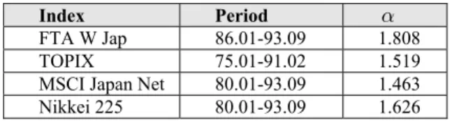
We analyze some results on financial data as reported by Lévy Véhel and Walter (LVW) [11] as well as from the PKDD 1999 discovery challenge financial database [12] in section 5.1. The importance of stable distribution is not only theoretical; as a matter of fact, it has far reaching consequences for financial data. With the pioneer work of Mandelbrot, it became increasingly apparent that financial data may be characterized with stable distributions. For instance, let us consider Table 1 which shows the results obtained for various Stock Market Indexes in Europe and in Japan by LVW [11]. The stability exponent was estimated with the method presented in Section 3 and the null hypothesis was asserted with the Kolmogorov-Smirnov test. As shown by the data, all these indexes clearly have a stable distribution (confidence level of 99%) and the value of the stability exponent is typically in between 1.6 and 1.8, which is clearly not in the Gaussian regime.
Table 2. Covariation of two shares (Thompson and Michelin) and the CAC 40 Index for various values of the stability exponent. and the acquisition period is from 87.07.09 to
95.05.31. Excerpted from [11]. 1, 2 X X a 2.0 a 1.7 1.5 1.3 THOMPSON, CAC 40 0.042 0.157 0.390 0.975 MICHELIN, CAC 40 0.042 0.159 0.326 0.993 CAC 40, CAC 40 0.036 0.128 0.300 0.750
Table 2 shows the covariations in between the Michelin and the Thompson titles as well as with the CAC 40 Stock Exchange Index. The covariations may be estimated with the method presented in Sections 4. The calculation was repeated for various values of the stability exponent; the real one being around 1.7. Table 2 shows that, if a Gaussian distribution is incorrectly assumed, the correlation (covariation) tends to be underestimated. For instance, the covariation in between the Michelin share and the CAC 40 Index is 0.042 with the false assumption of a Gaussian distribution for the data while in reality it is 0.159 for a stability exponent of 1.7. Here, the covariation tends to be stronger, when the stability exponent is smaller.
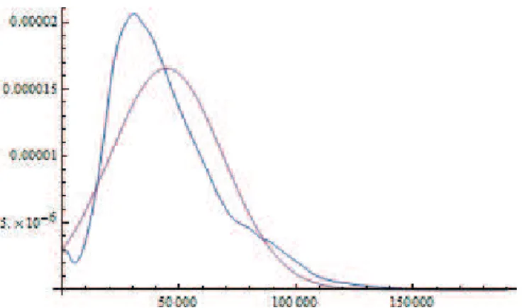
Fig. 1. Distribution of the Balance attribute (PKDD 1999 discovery challenge financial database) in blue and of the best fitting normal distribution in red; the later is obtained with the
maximum of likelihood method.
5.1 PKDD 1999 Discovery Challenge Financial Database
Next, we consider the PKDD 1999 discovery challenge financial database, which has been widely used as a benchmark in the multi-relational classification domain. This database was offered by a Czech bank and contains data describing the level of risk of a customer to default on a loan [12]. The database consists of eight tables. The Account table contains the account number, as well as the information regarding the district a person falls in and the frequency of payment. Other tables include the Demographic profile, the client’s Disposition in terms of type, Credit Card information and Client descriptions, including gender and the location in which they reside. The Order table details the number of money transfers and the Loan table describes the payments of loans. Very often, this database is used to classify whether a Loan is at risk or not.
We turn our attention to the Transaction table, which describes all transactions against an account. This table contains, amongst others, the Balance attribute that contains 54694 entries. We apply a number of feature selection algorithms to this database, including the Gain ratio, Chi Squared and Correlation based Feature Selection (CFS) measures [8]. Our results indicate that the Balance attribute is always
selected as being one of the features that are strongly related to the outcome of a Loan, with and without aggregation.
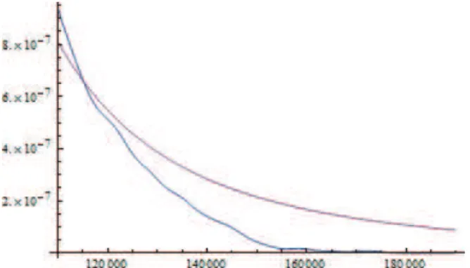
Figure 1 shows the distribution of the Balance attribute as well as the best fitting normal distribution. The parameters of the normal distribution are obtained with the maximum likelihood method. It follows that the normal distribution offers a poor fit to the Balance attribute distribution. We attempted to fit numerous distributions to the Balance such as the Student distribution, the Weibull distribution, amongst others. However, the best fit was obtained with the stable distribution, as illustrated in Fig. 2. The parameters corresponding to this distribution, which were obtained with the maximum likelihood method, are shown in Table 3. The tails of the Balance attribute distribution and the associated stable distribution are shown in Fig. 3. The tail of the fitted stable distribution seems thicker than the tail of the Balance attribute distribution: nevertheless, they both have the same order of magnitude. As may be observed from Fig. 3, the statistics of the tail is quite poor. This means that, in order to draw definitive conclusions about the tails, a database with more entries would be required.
Fig. 2. Distribution of the Balance attribute in blue and of the best fitting stable distribution in red; the later is obtained with the maximum of likelihood method.
Table 4 shows the mean, the standard deviation, the skewness and the kurtosis calculated from the normal and the stable distributions associated with the Balance attribute distribution. Since the stability exponent a is smaller than two, it is not possible to evaluate the standard deviation and the skewness from the stable distribution, because the statistical moments needed for the calculation are infinite.
TABLE 3. Parameters of the fitted stable distribution associated with the Balance attribute.
a b m g
1.6232 1.0 47321.3 14013.9
Nevertheless, the parameters of the stable distribution provide a measure of the standard deviation and of the skewness through the scale parameter g and b the asymmetry parameter. This implies that, when the underlying distribution is stable, the scale and the asymmetry should not be estimated directly from the data, but from the parameters of the fitted distribution.
Table 4. Mean, standard deviation, skewness and kurtosis as obtained from the fitted normal and stable distributions associated with the Balance attribute.
Distribution Mean Std Dev. Skewness Kurtosis
Normal 44534.2 24109.7 0 0
Stable 47321.3 ∞ ∞ ∞
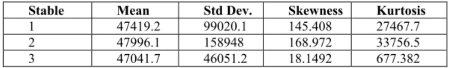
In order to further stress the importance of not directly estimating these parameters from the data, we have generated three data sets. These datasets consisted of 54694 entries as in the original bank database with the stable distribution parameterized by Table 4. Table 5 shows the results. Since the stability exponent is greater than one (1.62), the estimation of the mean from the data is consistent from one set to the next. However, because the stability exponent is less than two (1.62), it is not possible to estimate any moment greater or equal than two which means that the standard deviation, the skewness and the kurtosis are not consistent from one synthetic data set to the next. In other words, any measure based on the statistical moments greater or equal than two is a random number which will vary from one realization of the data set to the other as shown in Table 5. These findings suggest that when correlation evaluation is sensitive, say in privacy preservation learning, one should carefully select the right equation for correlation computation [8].
Table 5. Mean, standard deviation, skewness and kurtosis as obtained from data generated from the fitted stable distribution associated with the Balance attribute. Each generated data
set consists of 54694 entries.
Stable Mean Std Dev. Skewness Kurtosis
1 47419.2 99020.1 145.408 27467.7
2 47996.1 158948 168.972 33756.5
3 47041.7 46051.2 18.1492 677.382
6 Conclusions
The development of new data mining models for catastrophic event prediction, such as the damages caused by oil spills, stock market crashes, tsunamis and other natural disasters, are an important and urgent research topic. In this communication, we have analyzed data aggregation and the data covariance (covariation), of such data, where the underlying distributions are not Gaussian, but stable. We have shown that such data may be aggregated with the mean, but not with the variance. This is due
to the fact that the variance becomes infinite and its estimate tends to fluctuate randomly when evaluated on a finite size aggregate. We have also shown that the estimation of the mean converges rather slowly when the stability exponent is small. In this case, both the mean and the variance are infinite and their estimate on a finite size aggregate tends to fluctuate randomly. In these circumstances, the aggregate is better characterized with its maximum which tends to dominate by many orders of magnitude over the other elements of the aggregate, both from a sum and rank ordering statistics point of view. We have shown that financial data may be characterized with stable distributions with a stability exponent typically around 1.7. The calculation of the covariations in between Stocks and Stock Market Indexes has shown that the covariance (covariation) tends to be underestimated if a Gaussian distribution is wrongly assumed. We also shown that, for a well-known benchmarking financial database, some attribute values follow a stable distribution rather than the normal distribution. This work thus has implications when pre-processing and mining many highly imbalanced data that are typified with large-scale fluctuations, such as earthquake and oil spill data, which would be worth investigating further. We also mentioned, in Section 4, that our approach is highly relevant for correlation-based privacy preservation data mining. We aim to explore this research issue in our future work.
References
1. Knobbe, A., Siebes, A., Marseille, B.: Involving Aggregate Functions in Multi-Relational Search, Principles of Data Mining and Knowledge Discovery. LNCS, vol. 2431, pp. 145--168 (2002)
2. Malerba, D.: A relational perspective on spatial data mining. Int. J. Data Mining. Modelling and Management 1 ( 1), pp. 103--118 (2008)
3. Walter, C.: Lévy-stability-under-addition and fractal structure of markets: implications for the investment management industry and emphasized examination of MATIF notional contract. Mathematical and Computer Modelling 29 (10-12), pp. 37--56 (1999)
4. Groot, R. D.: Lévy distribution and long correlation times in supermarket sales. Physica A: Statistical Mechanics and its Applications 353, pp. 501--514 (2005)
5. Samorodnitsky, G., Taqqu, M. S.: Stable Non-Gaussian Random Processes: Stochastic Models with Infinite Variance. Chapman & Hall, New York (1994)
6. Paulson, A. S., Holcomb, E., Leitch, R.: The estimation of the parameters of the stable law. Biometrica 62 (1), pp. 163--170 (1977)
7. Nolan, J. P., Panorska, A. K., McCulloch, J. H..: Estimation of spectral measures. Mathematical and Computer Modelling 34 (9-11), pp. 1113--1122, (2001)
8. Guo, H., Viktor, H. L., Paquet, E.: Privacy Disclosure and Preserving in Learning with Multi-relational Databases. Journal of Computing Science and Engineering 5 (3), pp. 183-196 (2011)
9. Cheng, B., Rachev, S.: Multivariate Stable Future Prices. Mathematical Finance 5, pp. 133--153 (1995)
10. Tao, Y., Pei, J., Li, L., Xiao, X., Yi, K., Xing, Z.: Correlation hiding by independence masking. IEEE 26th International Conference on Data Engineering (ICDE). pp. 964--967, (2010)
11. Lévy Véhel, J., Walter, C.: Les marchés fractals ("The fractal markets"). Presses Universitaires de France, Paris (2002)
12. Berka, P.: Guide to the Financial Data Set. In A. Siebes and P. Berka, editors, PKDD 2000 Discovery Challenge (2000)