HAL Id: hal-03043430
https://hal.archives-ouvertes.fr/hal-03043430
Submitted on 7 Dec 2020
HAL is a multi-disciplinary open access archive for the deposit and dissemination of sci-entific research documents, whether they are pub-lished or not. The documents may come from teaching and research institutions in France or abroad, or from public or private research centers.
L’archive ouverte pluridisciplinaire HAL, est destinée au dépôt et à la diffusion de documents scientifiques de niveau recherche, publiés ou non, émanant des établissements d’enseignement et de recherche français ou étrangers, des laboratoires publics ou privés.
Shedding light on tectonic stress geometry in a key area
of seismic hazard
Sven Schippkus, Helmut Hausmann, Zacharie Duputel, Götz Bokelmann, _ _
To cite this version:
Sven Schippkus, Helmut Hausmann, Zacharie Duputel, Götz Bokelmann, _ _. The Alland earthquake sequence in Eastern Austria: Shedding light on tectonic stress geometry in a key area of seismic hazard. Austrian Journal of Earth Sciences = Mitteilungen der Oesterreichischen Geologischen Gesellschaft, Austrian Geological Society, 2019, 112 (2), pp.182-194. �10.17738/ajes.2019.0010�. �hal-03043430�
Abstract
We present our results on the fault geometry of the Alland earthquake sequence in eastern Austria (Eastern Alps) and discuss its implications for the regional stress regime and active tectonics. The series contains 71 known events with local magnitudes 0.1 ≤ ML ≤ 4.2 that occurred in between 2016 and 2017. We locate the earthquakes in a regional 3D velocity
model to find absolute locations. These locations are then refined by relocating all events relative to each other using a double-difference approach, based on relative travel times measured from waveform cross-correlation and catalogue data. We also invert for the moment tensor of the ML = 4.2 mainshock by fitting synthetic waveforms to the recorded seismo-grams using a combination of the L1- and L2-norms of the waveform differences. Direct comparison of waveforms of the largest events in the sequence suggests that all of them ruptured with very similar mechanisms. We find that the sequence ruptured a reverse fault, that is dipping with ~30° towards ~north-northeast (NNE) at 6–7 km depth. This is supported by both the hypocentres and the mainshock source mechanism. The fault is most likely located in the buried basement of the Bohemian massif, the “Bohemian Spur”. This (reverse) fault has a nearly perpendicular orientation to the normal-fault structures of the Vienna Basin Transfer Fault System further east at a shallower depth, indicating a lateral stress decoupling that can also act as a vertical stress decoupling in some places. In the west, earthquakes (at a larger depth within the upper crust) show compressive stresses, whereas the Vienna Basin to the east shows extensional (normal-faulting) stress. This provides insight into the regional stress field and its spatial variation, and it helps to better understand earthquakes in the area, including the “1590 Ried am Riederberg” earthquake.
earthquake; tectonics; moment tensor inversion; aftershocks; Eastern Alps
KEYWORDS
Zentralanstalt für Meteorologie und Geodynamik (ZAMG), Vienna, Austria
3) Institut de Physique du Globe de Strasbourg, Université de Strasbourg, EOST, CNRS, Strasbourg, France 4) www.alparray.ethz.ch
*) Corresponding author: [email protected]
1. Introduction
The Alps have a rich and complex tectonic history, induced by the convergence of the African and European plates (e.g., Jolivet et al., 2003; Schmid et al., 2004; Malusà et al., 2015) that is not fully understood yet (e.g., Lippitsch et al., 2003; Mitterbauer et al., 2011; Sun et al., 2019). The convergence is accompanied by an eastwards extrusion of crustal blocks of the Eastern Alps since the late Oligocene and early Miocene (Gutdeutsch and Aric, 1988; Ratschbacher et al., 1991; Wöl-fler et al., 2011; Barotsch et al., 2017). This lateral extrusion is associated with the formation of sinistral strike-slip faults in the north, in particular, the Salzach–Enns–Mariazell–Pu-chberg (SEMP; Fig. 1a) fault and the Mur–Mürz Line (MML; Fig. 1a) fault, as well as dextral strike-slip faults in the south, e.g., the Periadriatic Line and Lavanttal fault. Below these structures, we find the crystalline basement of the Bohe-mian massif and, further to the east, the Austroalpine base-ment under the Vienna Basin (Wessely, 2006). These two basement types have rather a different composition. The Bo-hemian massif is composed of magmatic rocks, whereas the Austroalpine basement is composed of metamorphic rocks (Wessely, 2006). Reinecker and Lenhardt (1999) argue that the “Bohemian Spur” (BS; see Fig. 1), the extent of the granit-ic basement of the Bohemian massif towards south, acts as an indenter, controlling the stress field in the Eastern Alps.
Understanding of this area, together with the entire Alpine region, can now be improved, due to the new dataset that is currently gathered by the AlpArray project (Hetényi et al., 2018). AlpArray is an international project of 55 institutions across Europe. It aims at advancing our understanding of the Alpine orogeny and surrounding regions with a previously unachieved dense coverage of the entire Alps with broad-band seismometers. In total, the network consists of almost 700 seismic stations, composed of ~240 newly installed temporary broadband stations, ~30 ocean bottom seis-mometers, and ~400 permanent stations.
The Alland earthquake sequence of 2016–2017 is located just near the eastern edge of the BS (red rectangle in Fig. 1c). Seismic activity is commonly observed in the south along the MML and southern part of the VBTFS (Fig. 1a), whereas it is more sparsely distributed to the north (Fig. 1c). Still, one of the most notable earthquakes in the region in the year 1590 (e.g., Gutdeutsch et al., 1987) has occurred in the same area (probably 20–30 km to the north) with a macroseismic magnitude of ~6 (see Fig. 1c). Hammerl (2017) reappraised this earthquake to possibly have happened ~10 km further towards east near Ried am Riederberg based on macro-seismic data points. This earthquake was the strongest his-torically documented earthquake in northeastern Austria, which has produced a significant damage in surrounding
determined if the dip angle is sufficiently small (Bukchin, 2006; Bukchin et al., 2010). The distribution of aftershock can provide additional information regarding the fault plane orientation (e.g., Rubin et al., 1999; Abercrombie et al., 2001; Bulut et al., 2007) and can help identify which of the two nodal planes has ruptured.
2. Data
The data used in this study consist of the seismic records of the Alland earthquake series recorded at 30 permanent stations (Czech Regional Seismic Network, 1973; Austri-an Seismic Network, 1987; HungariAustri-an National Seismo-logical Network, 1995; Seismic Network of the Republic of Slovenia, 2001; National Network of Seismic Stations of Slovakia, 2004) and 51 temporary broadband stations of the AlpArray seismic network (AlpArray Seismic Network, 2015) in distances of 20–250 km to the Alland main shock (see Fig. 1b). Thanks to the consistent station spacing throughout the network, stations are distributed evenly in azimuth. Data were downloaded using the ORFEUS web services (orfeus-eu.org).
3. Earthquake series characterization
The Alland earthquake sequence spanned ~1.5 years from April 2016 to November 2017 with 71 currently known events with ML ≥ 0.1, according to the AEC (2018). The events happened near the town of Alland, ~20 km southwest of Vienna in the Eastern Alps (red rectangle cities and villages, including Vienna. In the area
surround-ing the Alland earthquake sequence, only little seismic activity has been observed instrumentally in the past. According to the Austrian Earthquake Catalogue (AEC, 2018), there were only 13 documented earthquakes within a radius of 15 km around the Alland main shock since the year 1000: the largest with a macroseismic magnitude of ~4 in 1734 and none of the instrumentally recorded events exceeding magnitude 2.5. This makes the well-recorded Alland earthquake sequence and the information that can be gained from it particularly important. Earthquakes that have been detected along the MML and VBTFS consist mainly of strike-slip events, but there is also normal and reverse faulting (see Fig. 1c), reflecting the complex tectonic setting of the region.
In this study, we analyze locations and focal mechanisms of the Alland earthquake series to gain additional insight into the regional stress field. Furthermore, the Alland se-quence potentially illuminates the local fault geometry, which is only poorly known north of the MML and VBTFS due to the low seismicity of the region (see Fig. 1c). For this, we conduct two separate analyses that help con-strain the properties of the ruptured fault. We study the hypocentre distribution of the sequence and the source mechanism of the mainshock. While the source mech-anism gives insight into the rupture geometry, the de-tailed fault orientation of shallow earthquakes can be poorly constrained. The mechanism can only be uniquely
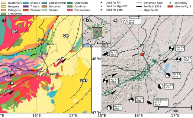
Figure 1: Map of the study region. a) Surface geology, extracted from the International Geological Map of Europe (IGME5000; Aschk, 2005). The thick
grey line marks the edge of the “Bohemian Spur” after Wessely (2006). The thick black line near the centre marks the location of the seismic profile C 8503 (Fig. 9). Major faults (dashed lines) are redrawn after Peresson and Decker (1997). Labelled faults: Alpine Front (AF), SEMP fault, Mur-Mürz-Line (MML), Vienna Basin Transfer Fault System (VBTFS). Labelled regions: Bohemian Massif (BM), Vienna Basin (VB), Eastern Alps (EA), and Little Hungarian Plain (LHP). b) Map of stations, classified by which parts of this study they are used in: moment tensor inversion (MTI), relocation with HypoDD, or both. c) Map of historical seismicity in the study region. Earthquakes are compiled from the Austrian Earthquake Catalogue (AEC, 2018) and the EMSC cata-logue (Godey, 2006). Source mechanisms are extracted from the ISC Bulletin (Lentas et al., 2019) and are provided by ZAMG. The red rectangle marks the zoomed-in view shown in Figure 3 and location of the Alland earthquake sequence. Thin grey lines mark the Austrian borders and city border of Vienna.
the increased station density in recent years, e.g., as part of the AlpArray project. The b-value – the negative slope of the Gutenberg-Richter plot, which indicates the rela-tive frequency of events with different magnitudes – is estimated as b ≈ 0.7 (Fig. 2b).
3.1 Locations
Accurate event locations can provide essential insight into the geometry and behaviour of fault systems. Rou-tine locations provided by ZAMG (Fig. 3a) use the data of the AlpArray and TU-SeisNet (gp.geo.tuwien.ac.at/gp/ tuseisnet) networks but are based on phase-arrival picks only. No fault structure seems to emerge from these lo-cations. This suggests that either the events are broadly distributed and not located on a single fault or there are large uncertainties in these locations.
To improve the absolute locations, we locate the events using NonLinLoc (Lomax et al., 2000; Apoloner et al., 2014) in a regional 3D velocity model (Behm et al., 2007). NonLinLoc performs a probabilistic, non-linear, global search for earthquake locations in the given model us-ing the eikonal finite-difference scheme of Podvin and Lecomte (1991). We find the events to be slightly more clustered and distributed along the discretized grid (Fig. 3b). Most notably, the largest events are now located ~2 km further towards northeast and the events are now in a slightly shallower depth, around 1 to 12 km.
in Fig. 1c), at depths of 4–12 km. Routine locations of the Alland series are available from the Austrian Seis-mological Service (Zentralanstalt für Meteorologie und Geodynamik, ZAMG), based on manual analysis of first P- and S-phase arrivals. The series seems to be divided into three sub-series that exhibit their own foreshock– mainshock–aftershock patterns (Fig. 2a).
The largest earthquake occurred on 25 April 2016 at 10:28:29 UTC with an estimated local magnitude of
ML = 4.2. This mainshock is part of the first sub-series of earthquakes (yellow dots in Fig. 2a), which includes 37 events of ML ≥ 0.1 that show a typical decay of after-shock rate with time (Omori, 1894). After five days of no activity, the second sub-series (blue dots in Fig. 2a) with 20 events took place, including its largest event on 10 May 2016 with ML = 2.8. Scattered throughout the fol-lowing 2 months, there was little activity with five events with ML < 2 (white dots in Fig. 2a). Then, after 463 days of no activity, the third sub-series (green dots in Fig. 2a) occurred with nine events, including the second-largest event of the series on 9 November 2017 with ML= 3.2. For the complete sequence, we estimate the magnitude of completeness MC, which is the lowest magnitude above which all events are detected, MC≈ 1.0 (Fig. 2b), which is similar to the one estimated for the AEC from 1995 to 2018 (MC ≈ 1.4, H. Hausmann, pers. comm.). A slightly lower MC in this sequence may be attributed to
Figure 2: Properties of the Alland earthquake sequence. a) time history of the Alland earthquake series. The main shock occurred on 25 April 2016 with
an estimated local magnitude of 4.2. We distinguish the series into three sub-series (marked by yellow, blue, and green colors). There is a 463 day gap from 1 August 2016 to 8 November 2017 with no measured seismic activity in the area. b) Gutenberg–Richter plot of the Alland series. We find a b-value of 0.7 and estimate the magnitude of completeness MC ~ 1.0.
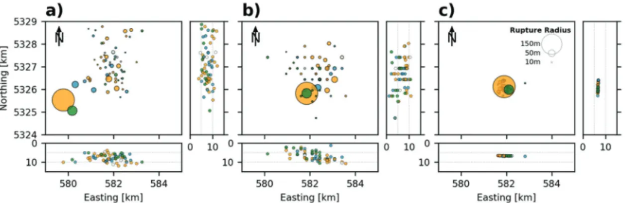
Figure 3: Locations of the earthquakes from the a) Austrian Earthquake Catalogue (AEC, 2018), b) NonLinLoc, and c) HypoDD. Circle sizes scale with the
estimated rupture dimension; the drawn circle radii are three times the rupture radii. Circle colours are as shown in Figure 2. The coordinate system is UTM32N; see Fig. 1 for the location of this zoomed view. While the NonLinLoc locations show slightly increased clustering of the events, the locations retrieved with HypoDD cluster very well in a narrow area.
and the computational cost is low. After testing several parameter settings, we decide to use four sets of four it-erations, each with successively stricter residual thresh-old (residual threshthresh-old for cross-correlations (WRCC) and catalogue data (WRCT) = none, 5 s, 3 s, and 2 s) and maximum distance between linked pairs (distance threshold for cross-correlations (WDCC) and catalogue data (WDCT) = none, none, 5 km, and 3 km). The velocity model we use for relocation is the mean model extracted from Schippkus et al. (2018), assuming a vp /vs ratio of √3. All 68 events are automatically assigned to the same cluster by HypoDD.
The locations found with HypoDD are much more densely clustered than the previous locations (Fig. 3c), with estimated location errors less than 10 m (see Elec-tronic Supplement). Most events are located to the southeast of the mainshock, and all events are at a shal-lower depth (~6.5–7.0 km) than the previously inferred locations, with the mainshock at 6.7 km depth (Fig. 3c). All events seem to fit on a single fault plane, allowing us to fit a plane through the new locations of all events with
ML > 0.2 (Fig. 4a). The three events with ML ≤ 0.2 are
ap-parently too weak to be well located, as they have a low SNR and are recorded on only a few nearby stations, and thus they are excluded. We find an excellent match of the remaining events with that of the plane. The mean mis-fit is 20 m, and there is no deviation larger than 152 m. To better illustrate the fit, we present a down-dip view and a side view of the plane (Fig. 4b). The plane has a strike of 299° and dips towards NNE with a dip angle of 26° from horizontal.
Most aftershocks do not cluster in the immediate vi-cinity of the mainshock (Fig. 4c), suggesting that most of them do not overlap with the co-seismic rupture area of the mainshock. They are more distributed to-wards the edge and outside the main shock rupture area. Inter-event distances (Fig. 4d), i.e., the distance of a given event from the next one, can be interpreted to give an estimate of rupture size (Rubin et al., 1999) as it is unlikely for an aftershock to occur within the rupture area of its mainshock (Mendoza and Hartzell, 1988). Assuming a circular crack model, we can esti-mate the stress drop ∆s by r = (7M0/16∆s)1/3 (Eshelby,
1957), with the rupture radius r and the seismic mo-ment M0. Abercrombie (1996) gave an empirical rela-tion between local magnitude ML and seismic moment
= +
M0 101.0 9.8ML, which we apply here. We estimate a
stress drop of ∆s = 10 MPa (dashed line in Fig. 4d) for the larger events, as there is no event below the dashed line (Rubin et al., 1999). This stress drop is larger than the global average of 3 MPa, but it is consistent with the fact that intra-plate earthquakes are often associ-ated with a larger stress drop (Allmann and Shearer, 2009). Circle sizes in Figures 3 and 4c are based on these estimated fault dimensions. The new locations from NonLinLoc and HypoDD are attached as a table in the Electronic Supplement.
Using these improved absolute locations as the initial locations, we relocate the events in this series relative to each other. Taking a double-difference approach to determine relative locations of nearby and similar events has been repeatedly shown capable to provide precise estimates of the rupture geometry; it is a well- established procedure (e.g., Prejean et al., 2002; Schaff et al., 2002; Waldhauser and Schaff, 2008). The approach is based on the assumption that differences in trav-el times measured for nearby events are only caused by a change in location, as the path effects are essen-tially the same. We use the HypoDD software package (Waldhauser and Ellsworth, 2000; Waldhauser, 2001) to find improved relative locations. With this approach, 68 of the 71 known events in this series are relocated. Three events are excluded, because they occurred with-in only 16 seconds and their waveforms overlap heavily. On these waveforms, we cannot easily distinguish the different phases of the three events.
We use both waveform cross-correlation as well as travel times from the catalogue (ZAMG) to estimate rel-ative arrival times for all event pairs. Relrel-ative time shifts from cross-correlation are measured for P- and S-phases separately in time windows around the theoretical first P- and S-arrivals, computed by ray tracing (Crotwell et al., 1999) in a 1D medium (Kennet, 1991). The P-phase time window is defined as 2 seconds before and 6 sec-onds after the first theoretical arrival. For the S-phase, we use 2 seconds before and 12 seconds after. Some stations require static time corrections (up to 3 sec-onds), because the 1D model does not account for lat-eral heterogeneities and therefore the theoretical phase arrivals are not always properly aligned with the actual arrivals in the seismograms (see Fig. S1). We bandpass filter the data from 5 Hz to 15 Hz to ensure high signal-to-noise ratio (SNR) for all event magnitudes and ex-clude all waveforms with SNR <10. Here, we define SNR as the ratio of peak amplitude to standard deviation of noise, where the noise window is in between the source time and the first theoretical P-arrival. For each station pair, we shift the filtered waveforms towards the high-est cross-correlation coefficient, which also acts as the weight given to the measurement during the relocation process (see Fig. S2). To ensure high data quality, we al-low only measurements where the estimated relative P- and S-arrivals match roughly (i.e., they are within 10% of each other). We retrieve a total of 17,939 relative P- and 17,939 relative S-arrival times from waveform cross-correlation. The catalogue-based relative travel times for P- and S-phases are initially weighted with 0.01, because manual phase picks are generally less precise than waveform cross-correlations and are sub-ject to human error. There are 3,235 relative P- and 2,913 relative S-arrival times available.
In HypoDD, we use the singular value decomposition mode (Waldhauser and Ellsworth, 2000) to solve for rel-ative locations, because the data set is relrel-atively small
physically unreasonable amplitudes, most likely caused by incorrect instrument response information.
To reduce computational cost, the parameter space is confined by excluding equivalent plane solutions, i.e., we limit strike to 180°–360°. We sample the parameter space with 5° spacing in strike, dip, and rake during the first two it-erations, and increase the grid density to 1° spacing for the last three iterations to converge to a more precise solution.
We use bandpass-filtered waveforms in the frequency band from 0.02 Hz to 0.05 Hz to estimate the waveform fit. In this band, we do not expect the seismic wave propaga-tion to be heavily influenced by local geological hetero-geneities, i.e., the waves are dominated by source- rather than path- or site-effects. Therefore, we deem comput-ing the synthetic waveforms in a 1D model appropri-ate, given that we allow the waveforms to shift in time. We decided on the 0.02–0.05 Hz frequency band to have the waveform fit be insensitive to local heterogeneities. This also reduces the amount of information that needs to be fit, for a lower computational cost. The downside of this choice is that the iterative approach eliminates more channels if the periods used are relatively long, because not all stations have good-quality long-period records on all components. This affects especially the horizontal channels of the temporary stations of the AlpArray proj-ect. A total of 36 channels (27 Z, 7 R, 2 T) are used in the final iteration to compute the best-fit solution.
3.2 Deriving the source mechanism
We determine the source mechanism of the main-shock (ML= 4.2 on 25 April 2016) by grid searching the double-couple (DC) parameter space for the best fit with synthetic waveforms. The synthetic waveforms for each combination of strike, dip, and rake are computed by modal summation using the Computer Programs in Seis-mology (Herrmann, 2013) in a 1D model (Kennet, 1991) for all source-station distances and back azimuths, as well as a range of depths.
To evaluate the waveform fit, we follow the approach presented in Zhu and Helmberger (1996), which builds upon Zhao and Helmberger (1994) by fully using the amplitude information. The approach combines L1- and L2-norms of the displacement-waveform differences, where the waveforms are allowed to be shifted in time towards the best fit to account for regional geologi-cal deviations from the 1D model (for more details, see Supplement Text S1). This approach to misfit estimation is susceptible to strong biases by faulty/noisy channels, because there are no inherent quality checks performed on the data and the full waveform is utilized. Therefore, we take an iterative approach to finding the best solution for each depth, similar to Duputel et al. (2012), in which we run multiple iterations with an increasingly stricter waveform selection (for more details, see Supplement Text S2). For the first run, we remove only channels with
Figure 4: Final relative locations of the Alland earthquake series. a) Oblique 3D view towards northwest of the hypocenter locations after relocating the
event series with HypoDD, and the best-fitting plane through all events ML > 0.2 with strike 299° and dip 26° (black mesh). b) Down-dip and side views
of the plane to illustrate the fit. c) Fault-projected view of inter-event distances with circle sizes representing the estimated rupture areas. d) Inter-event distances, i.e., the distance from one event of a given magnitude to the next one in time. The dashed line represents the modelled rupture radius, which is used in c), assuming a stress drop of σ = 10MPa All arrows mark north. Circle colours are as shown in Figure 2.
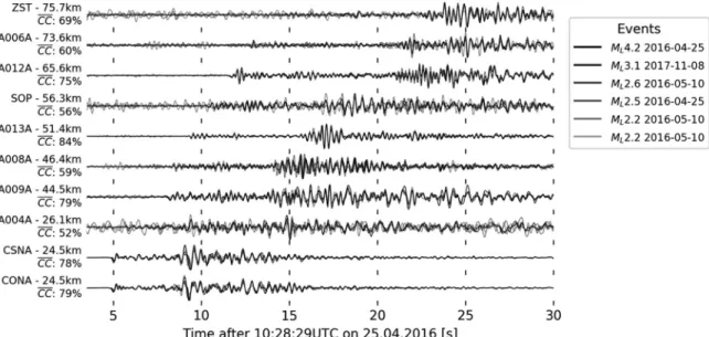
the synthetic waveforms without full knowledge of the subsurface structure (Šilený, 2004). Instead, we direct-ly compare the seismograms of the six largest events (2.2 ≤ ML ≤ 4.2), recorded on the vertical components
(bandpass filtered 0.5–5 Hz) of the ten closest stations to the source (Fig. 6). We find a remarkable similarity of these waveforms (mean cross-correlation coefficients CC with the mainshock from 52% to 84%; Fig. 6). This clearly suggests that the mechanisms for the largest aftershocks are very similar to those for the main shock.
4. Discussion
We have studied locations of the Alland earthquake sequence and the orientation of the main shock, and we have seen that the earthquakes occurred on a rath-er well-defined planar surface in the basement, which agrees fairly well with (one of the possible) fault planes of the Alland main shock (Fig. 5c). We will discuss this, starting with the robustness of our results and later put-ting them into the geological/tectonic context of the region. The hypocentre location errors from HypoDD in all three dimensions are small, usually well below 10 m (see Electronic Supplement). The depth determined from the source mechanism, on the other hand, is only poorly constrained. The misfit found at depths from 5 to 9 km depth is within only 5% of the misfit at 7 km depth (Fig. 5a). We do not claim this difference in wave-form fit to be significant enough to make statements about source depth from the source mechanism alone. Still, the best-fit depth corroborates the depth found by relocation (6.7 km, Figs. 3c and 4, Electronic Supple-ment). Similarly, the fault planes found from aftershock hypocentres (strike 299° and dip 26°, Fig. 4) and the mainshock source mechanism (strike 317°, dip 40°, rake 101° or equivalently strike 123°, dip 51°, rake 81°; Fig. 5) agree fairly well, although the dip towards NNE/NE We compute the best-fit solution for depths from 1 km
to 13 km in 2 km steps (Fig. 5a) to get additional con-straints on the depth of the mainshock that may reassure our findings from relative relocation. The best waveform fit is found for a source at 7 km depth. All depths from 5 km to 9 km show misfits within 5% of the lowest misfit. A reverse-faulting solution is preferred for all depths from 3 km to 13 km, and only at 1 km depth, a strike-slip solu-tion is found, although with a considerably higher error (+11%). There the solution is based only on five remain-ing waveforms in the final iteration, and the mechanism is likely not well determined in these very shallow depths (Bukchin, 2006; Bukchin et al., 2010). We test the influ-ence of the frequency band on our results and find that reverse-faulting solutions are preferred for all tested fre-quency bands at 7 km depth (Fig. 5b), although the best-fit strike changes between NW/SE- and W/E-orientations, depending on the band.
Three slices crossing the DC parameter space for the best-fit source mechanism with a source depth of 7 km show a stable solution that is well defined in the rake-strike, rake-dip, and dip-strike planes (Fig. 5c). We find that the main shock ruptured as a slightly oblique reverse-faulting event on either a plane with strike 317°, dip 40°, and rake 101°, or on the equivalent plane with 123° strike, 51° dip, and 81° rake. The moment magnitude MW = 3.7 is estimat-ed from the mean seismic moment (Hanks and Kanamori, 1979) measured over all 36 channels that were used in the last iteration (see Fig. S3).
The waveform fit with synthetics for smaller events in the series, e.g., the ML = 3.2 earthquake, on 9 November 2017 proved to be unstable, which is not surprising. Be-cause of the lower magnitude and thus reduced exci-tation of long-period waves, higher frequencies have to be utilized. These are more sensitive to structural hetero-geneities, which leads to inaccuracies due to computing
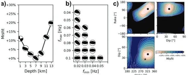
Figure 5: Results of the moment tensor inversion. a) Depth dependence of the mainshock source mechanism. In most depths, a reverse-faulting
mech-anism is preferred and the lowest misfit is found at 7 km depth. b) Frequency-band dependence of the best-fit source mechmech-anism at 7 km depth. In all tested frequency bands, a reverse-faulting mechanism is preferred. The strike of the preferred rupture plane varies NW–SE to W–E for higher frequencies. c) Slices through the solution space, crossing the best-fit solution (•) for 7 km depth and 0.02–0.05 Hz frequency band for the last iteration, estimated on the 36 remaining waveforms. [] marks the orientation of the plane fit through the earthquake hypocentres (see Fig. 4).
This is further supported by the two other fault plane solutions of the Alland mainshock that are available from ZAMG (Freudenthaler, pers. comm.) and Saint Louis Uni-versity Earthquake Center (Saint Louis UniUni-versity, 2016). The solution provided by ZAMG is based on manual analysis of first P-arrivals, as well as polarities and SV to P amplitude ratios (Fig. 7, left), whereas the automatically generated solution by Saint Louis University (SLU; Fig. 7, centre) is based on fitting waveforms with synthetics, similar to our approach. We find good agreement of our results with the solution reported by ZAMG (strike 324°, dip 41°, rake 105°), while the solution reported by the SLU (strike 348°, dip 46°, rake 144°) deviates from our findings, mostly in rake. We speculate that this is the case, because the SLU solution is based on only permanent stations that are preferentially distributed towards north and south, and not all waveforms used for the determination of the source mechanism have high cross-correlation co-efficients with the synthetics (as low as 4%, Saint Louis University, 2016). Nonetheless, the SLU solution seems to lie within +5% misfit of our best-fit solution (Fig. 5c).
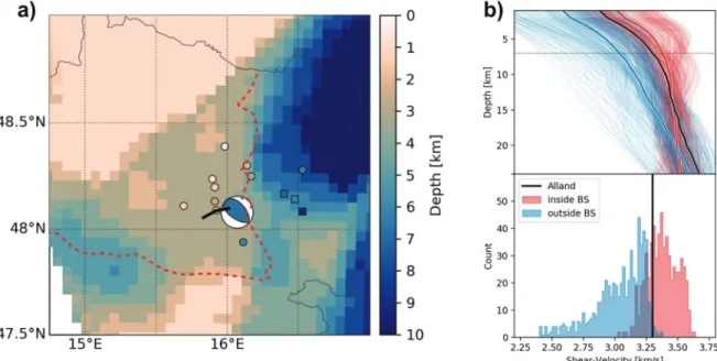
The Alland earthquake sequence ruptured a fault that is located near the eastern edge of the BS at depths of 3–4 km below the crystalline basement top (Fig. 8a). In Figure 8a, we show the first depth at which the shear- velocity model of Schippkus et al. (2018) exceeds 2.9 km/s. Schippkus et al. (2018) argued that the 2.9 km/s isosur-face is a good representation of the crystalline basement top. We compare these depths with basement depths known from boreholes and interpret from geological profiles (Fig. 8a), as well as the shape of the BS as drawn in Wessely (2006) (dashed line in Fig. 8a). We find reason-able agreement between these observations. An import-ant question for the understanding of this sequence is differs by 14°. When looking at solutions that are within
5% misfit of the best-fit source mechanism (first contour line in Fig. 5c), we cannot confidently distinguish solu-tions over a relatively wide range in strike (~290°–340°) and dip (~30°–45°), and an interdependence of strike and rake is apparent. We show only three planes cross-ing the global minimum in the 3D parameter space that can only give limited insight into the distribution of mis-fits in the full parameter space. Still, it seems that the dip angle is constrained better than strike and rake (Fig. 5c). We can therefore consider the two found planes to be consistent with each other; they have a Kagan angle of 18° (Kagan, 1991). Still, the fault plane orientation seems to be better constrained by the aftershock hypocentres. While the fault orientation rotates towards E–W striking at higher frequencies (Fig. 5b), the two independent analyses of the fault plane orientation match better at the lower frequencies used in this study, suggesting that small-scale geological heterogeneities may indeed bias the results of the moment tensor inversion at higher frequencies.
Figure 6: Overlaid waveforms (vertical component) of the six largest events (ML > 2) in the series, bandpass-filtered 0.5–5 Hz and shifted towards the best fit on the 10 closest stations. A strong similarity between aftershock waveforms with the main shock (mean cross-correlation coefficients CC between 52% and 84%) suggests similar source mechanisms and locations for all of these events.
Figure 7: Fault plane solutions. Left: 323°/41°/105° from
Zentralan-stalt für Meteorologie und Geodynamik (ZAMG) based on first P-, SH-, and SV-arrival polarities (Freudenthaler, pers. comm.). Center: 348°/46°/144° from Saint Louis University Earthquake Center based on waveform fitting with synthetics using only permanent stations that are preferentially distributed towards North and South (Saint Louis University, 2016). Right: 317°/40°/101° from this study.
to the buried BS appears quite possible; this could then result in a favourable alignment of one of these faults, so that it might have been reactivated by reverse faulting.
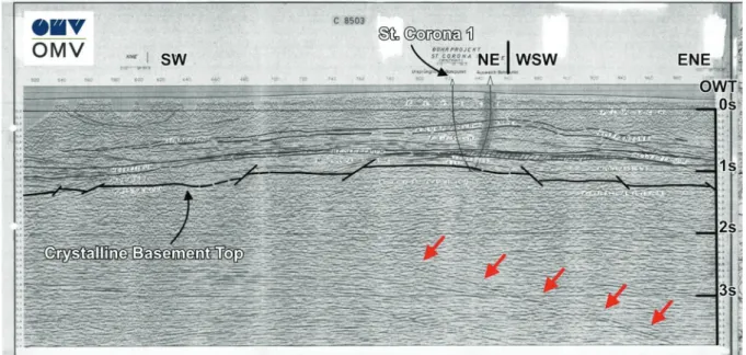
The seismic reflection profile C 8503, kindly provided by OMV Aktiengesellschaft, crosses the nearby borehole St. Corona 1 and runs in close proximity to the Alland se-quence epicentres (Fig. 9); the eastern end of the profile is located in ~7 km distance. The borehole gives ground truth for the top of the crystalline basement in 2.6 km depth (at ~1 s one-way-travel (OWT) time in the profile). Below, in the crystalline basement, there is an extensive ~NE-dipping reflector visible at ~3 seconds OWT (red ar-rows in Fig. 9), corresponding to depths of ~6–7 km. This profile confirms the presence of major ~NE-dipping fea-tures in the crystalline basement, in depths consistent with the fault plane of the Alland sequence (see Figs. 4 and 5).
The Alland sequence ruptured the fault with a reverse mechanism, which is not uncommon in the area. The Seebenstein ML = 3.6 earthquake of 25 January 2013 was a reverse-faulting earthquake with a rather similar source geometry to that of the Alland earthquake (see Fig. 1) and at a similar depth (10 km from AEC, 2018). On 16 April 2019, an ML= 3.1 earthquake occurred about 40 km to the north, near Tulln (April 2019 seismicity report by ZAMG) in a previously seismically quiet area, which potentially ruptured more shallow rocks (9 km depth from ZAMG) with a reverse-faulting mechanism where exactly the edge of the BS is located and whether
the ruptured fault is located in the granitic basement of the Bohemian massif or in the metamorphic Austroalpine basement to the east. The velocity model of Schippkus et al. (2018) seems to suggest a shape of the BS similar to that in Wessely (2006) (dashed line in Fig. 8a). We ex-tract shear-velocity profiles from the model of Schippkus et al. (2018) in the study area and classify them as being located “inside” or “outside” the BS, following the interpre-tation of Wessely (2006) (Fig. 8b). We find that the velocity profile near Alland (black line in Fig. 8b, top) more close-ly resembles the mean velocity profile inside the BS (red line in Fig. 8b, top). The RMS misfit between these two profiles is 0.08 km/s compared to 0.21 km/s for the mean velocity profile outside the BS (blue line in Fig. 8b, top). The distribution of velocities at 7 km depth, the source depth of the Alland sequence, further illustrates that the shear velocities found near Alland (black line in Fig. 8b, bottom) match the distribution of velocities inside the BS (red histogram in Fig. 8b, bottom) better.
Therefore, it seems very likely that the Alland sequence ruptured the crystalline basement of the Bohemian mas-sif and not the Austroalpine basement. In the Bohemi-an massif, a criss-cross pattern of SSW/NNE- as well as SSE/NNW-striking strike-slip faults is well documented (e.g. Brandmayr et al., 1995), which have shown only little activity recently. A continuation of this fault pattern down
Figure 8: Regional context of the Alland earthquake. a) Alland earthquake near the edge of the Bohemian Spur (BS). Background image shows the first
depth at which 2.9 km/s shear velocity is exceeded in the velocity model of Schippkus et al. (2018), which may be interpreted as the top of crystalline basement (see Schippkus et al., 2018 for more details). Crystalline basement depths, known from boreholes (marked as ) or estimated from geological profiles (marked as ¨) from Wessely (2006). The beachball represents the Alland main shock, also coloured by depth. Red line marks the edge of the BS, redrawn from Wessely (2006). Black line marks the seismic profile C 8503 that crosses the borehole St. Corona 1 (see Fig. 9). b) Velocity model of Schippkus et al. (2018), classified by “inside” (red colour) and ‘outside’ (blue colour) the BS after Wessely (2006). Classification is based on the edge of the BS as drawn in Figures 1 and 8a. Top: velocity profiles, extracted at each grid node in a), extracted from Schippkus et al. (2018). Thick lines represent the mean velocity profiles inside (red) and outside (blue) the BS. The velocity profile at the location of the Alland sequence is drawn in black. The Alland profile (black) is similar to the mean velocity profile inside the BS (red). Bottom: Histogram of shear velocities at 7 km depth (source depth of Alland main shock, dotted line in top panel). Clear separation of faster and slower velocities by the classification with some overlap. The shear velocity found in 7 km depth near the Alland series (black line) appears more likely to be representative of the BS (red distribution).
which would render the observed source mechanism of the Alland main shock highly unlikely, if the ruptured fault has not been extensively weakened in the past. The lack of previous seismicity on this fault may perhaps sug-gest that it has not been weakened. If the rotation of sH-
orientation around the BS was not representative of the regional stress field and instead SSW/NNE orientations were also present just southeast of the BS, that would fur-thermore render the southern Vienna Basin Transfer Fault System (VBTFS in Fig. 1a), as well as the MML (Fig. 1a) nearly optimally oriented, as strike-slip faults. Indeed, larger-scale studies (e.g., Robl and Stüwe, 2005; Bada et al., 2007; Heidbach et al., 2016) also show a coherent SSW/NNE orientation of sH in the Vienna basin.
This leads us to speculate that the mountain- range- perpendicular sH orientation, rotating along the
Alpine front and observed elsewhere, e.g., in Bavaria and Switzerland (Reinecker et al., 2010; Heidbach et al., 2016), also holds for eastern Austria. This may indicate that a buoyancy- rather than rheology-driven stress field (as sug-gested in Reinecker and Lenhardt, 1999) may be important, but to substantiate this is beyond the scope of this paper.
The tectonic regime in the adjacent Vienna basin is ob-viously a different one compared with that in the BS and west of it; it is dominated by strike-slip and normal fault-ing. It may be surprising that the tectonic regime can vary over distances of just tens of kilometres. There have been suggestions before though that the stress field in the Vienna basin differs from that in the basement below. In particular, the Steinberg fault (e.g., Lee and Wagreich, 2016) seems to be the place of a major change in the orientation of the stress field (Marsch et al., 1990; Decker et al., 2005).
that may have been oriented similar to the Alland earthquake (C. Freudenthaler, pers. comm.). There were reverse-fault events dispersed throughout the Northern Calcareous Alps (C. Freudenthaler, pers. comm.), and they may possibly also have occurred in eastern Switzerland (Strasser et al., 2006). These observations in combination with the results presented in this paper make it clear that reverse faulting is an important rupture mechanism in the Eastern Alps and along its eastern edge.
These consistent larger-scale observations are likely driven by the regional stress field. The Alland earthquake with a moment magnitude MW = 3.7 therefore also sheds light on the regional stress field and thus into the forc-es that drive tectonic deformation in the area today. The source area of the main shock is about 400 m long (see Fig. 4c); due to this extended size, the earthquake is prob-ably more representative of the regional stress field than borehole-derived stress indicators that relate to small spatial scales and usually to shallower levels in the crust. The source mechanism of the main shock and aftershock locations indicates that the maximum horizontal com-pressive stress sH is oriented ~30° from north over east
in the upper crust near the edge of the BS. The dip of the fault plane is around 26–40° from the horizontal (see Figs. 4 and 5), a nearly optimal orientation for a reverse fault. This also supports the Alland earthquake as an im-portant indicator for the regional stress field in this re-gion, where we have little information on crustal stress.
The study of Reinecker and Lenhardt (1999) implies that this reverse-faulting stress regime with an SSW/NNE orientation of sH is prevalent in the region to the west
of Alland, as far as Salzburg. Near the eastern edge of the BS, however, they report SSE/NNW sH-orientations,
Figure 9: Seismic reflection profile C 8503, provided by OMV. The profile crosses the borehole St. Corona 1, which reached the crystalline basement at
2.3 km depth, corresponding to 1 s OWT time in the profile. The Alland sequence ruptured a fault at 6–7 km depth (~3 s OWT). At these depths, the pro-file reveals an extensive ~NE dipping feature in the crystalline basement (indicated by red arrows). The eastern end of the propro-file is located ~7 km from the Alland main shock (see Fig. 8). This profile confirms the presence of major ~NE-dipping features in the crystalline basement of the Bohemian Massif, roughly consistent with the fault orientation of the Alland sequence (see Figs. 4 and 5).
et al. (2000), Herrmann (2013), and Krischer et al. (2015). Part of this work was performed using funding from the Austrian Science Fund (FWF): Projects 26391 and 30707. The authors thank the Austrian Agency for International Cooperation in Education & Research (OeAD-GmbH) for funding the Amadée project FR02/2017, which helped directly facilitate work on this project. This project was co-funded by the French Europe & Foreign Affairs try and the French Higher Education and Research Minis-try under the project number PHC-AMADEUS 38147QH. Thanks to OMV for insightful discussions and providing the seismic reflection profile C8503. Thanks to the Cen-tral Institute for Meteorology and Geodynamics, Vien-na, Austria (ZAMG), for providing their focal mechanism solution for the 2015 Alland and 2019 Tulln main shocks. We thank the Alparray Seismic Network Team: G. Hetényi, R. Abreu, I. Allegretti, M.-T. Apoloner, C. Aubert, S. Besançon, M. Bès De Berc, G. Bokelmann, D. Brunel, M. Capello, M. Čarman, A. Cavaliere, J. Chèze, C. Chiarabba, J. Clin-ton, G. Cougoulat, W. C. Crawford, L. Cristiano, T. Czifra, E. D’alema, S. Danesi, R. Daniel, A. Dannowski, I. Dasović, A. Deschamps, J.-X. Dessa, C. Doubre, S. Egdorf, ETHZ-Sed Electronics Lab, T. Fiket, K. Fischer, W. Friederich, F. Fuchs, S. Funke, D. Giardini, A. Govoni, Z. Gráczer, G. Gröschl, S. Heimers, B. Heit, D. Herak, M. Herak, J. Huber, D. Jarić, P. Jedlička, Y. Jia, H. Jund, E. Kissling, S. Klingen, B. Klotz, P. Kolínský, H. Kopp, M. Korn, J. Kotek, L. Kühne, K. Kuk, D. Lange, J. Loos, S. Lovati, D. Malengros, L. Margheri-ti, C. Maron, X. Martin, M. Massa, F. Mazzarini, T. Meier, L. Métral, I. Molinari, M. Moretti, H. Munzarová, A. Nardi, J. Pahor, A. Paul, C. Péquegnat, D. Petersen, D. Pesaresi, D. Piccinini, C. Piromallo, T. Plenefisch, J. Plomerová, S. Pondrelli, S. Prevolnik, R. Racine, M. Régnier, M. Reiss, J. Ritter, G. Rümpker, S. Salimbeni, M. Santulin, W. Scherer, S. Schippkus, D. Schulte-Kortnack, v. Šipka, S. Solarino, D. Spallarossa, K. Spieker, J. Stipčević, A. Strollo, B. Süle, G. Szanyi, E. Szücs, C. Thomas, M. Thorwart, F. Tilmann, S. Ueding, M. Vallocchia, L. Vecsey, R. Voigt, J. Wassermann, Z. Wéber, C. Weidle, v. Wesztergom, G. Weyland, S. Wiemer, F. Wolf, D. Wolyniec, T. Zieke, and M. Živčić.
References
AEC, 2018. Austrian Earthquake Catalogue from 1000 to 2018 A.D., Unpublished computer file, Zentralanstalt für Meteorologie und Geodynamik, Section Seismology, Division Data, Methods, Modeling, 1190 Wien, Hohe Warte 38, Austria
Abercrombie, R.E., Bannister, S., Pancha, A., Webb, T.H., Mori, J.J., 2001. Determination of fault planes in a complex aftershock sequence using two-dimensional slip inver-sion. Geophysical Journal International, 146, 134–142. https://doi.org/10.1046/j.0956-540x.2001.01432.x Allmann, B.P., Shearer, P.M., 2009. Global variations of
stress drop for moderate to large earthquakes. Journal of Geophysical Research: Solid Earth, 114/24, 015–22. https://doi.org/10.1029/2008JB005821
5. Conclusions
We provide information about the geometry and be-haviour of the fault involved during the Alland earth-quake sequence in eastern Austria. This earthearth-quake sequence occurred from April 2016 to November 2017 and includes 71 known events; its largest event has a mo-ment magnitude of MW = 3.7. Our source mechanism indi-cates that this event ruptured a reverse fault with a strike of 317° and a dip of 40°, which is fairly consistent with the distribution of relocated aftershock hypocentres that fit on a plane with strike 299° and dip 26°. The six largest events (ML > 2) show a high waveform similarity with the main shock, suggesting that these events ruptured with similar reverse-fault mechanisms. Earthquake relocation indicates that the sequence occurred at around 6.5–7 km depth with the mainshock at 6.7 km, which is in agree-ment with the best point-source depth of our moagree-ment tensor inversion.
The ruptured fault is located near the eastern edge of the BS, the extent of the crystalline basement of the Bo-hemian Massif towards south, at depths of a few kilome-tres below the overthrust Alpine nappes. The sequence has most likely ruptured the granitic basement of the Bohemian massif and potentially a pre-existing fault. A previously unpublished seismic profile in the vicinity provides evidence for the existence of such faults in the basement. The Alland earthquake sequence suggests that the maximum horizontal stress sH in the upper crust
in this region may be oriented normal to the Alps, which has also been observed in the Western and Central Alps before, resulting in a ~NNE/NE orientation of sH at the
eastern edge of the Eastern Alps. Thus, reverse faulting is an important rupture mechanism in the Eastern Alps. This suggests that the stress field in the vicinity of the Alps is likely affected by buoyancy, caused by the higher eleva-tion of the Alps and the Bohemian Massif, and possibly by lateral density variation, e.g., by crustal roots. The orien-tation of the stress field in the basement seems to be dif-ferent from the one in the adjacent (and partly overlying) Vienna Basin, and the basin-bounding faults seem to be effective in decoupling the two stress fields. The Alland earthquake, the recent 2019 Tulln earthquake, and po-tentially also the M ≈ 6 Ried am Riederberg earthquake of 1590 have responded to the compressive basement stress field.
Acknowledgements
We thank the editor (Kurt Stüwe) and two reviewers (Stefanie Donner and anonymous) for constructive com-ments that helped improve the manuscript. The data used in this study are provided by the operators of the nation-al seismic networks (Czech Regionnation-al Seismic Network, 1973; Austrian Seismic Network, 1987; Hungarian Nation-al SeismologicNation-al Network, 1995; Seismic Network of the Republic of Slovenia, 2001; National Network of Seismic Stations of Slovakia, 2004) and the members of the AlpAr-ray Working Group (AlpArAlpAr-ray Seismic Network, 2015). The software used in this study was kindly provided by Lomax
305–320. https://doi.org/10.1016/j.quascirev.2004.04.012 Duputel, Z., Rivera, L., Kanamori, H., Hayes, G., 2012.
W phase source inversion for moderate to large earth-quakes (1990-2010). Geophysical Journal International, 189, 1125–1147, Oxford University Press. https://doi. org/10.1111/j.1365-246X.2012.05419.x
Eshelby, J.D., 1957. The Determination of the Elastic Field of an Ellipsoidal Inclusion, and Related Problems. Pro-ceedings of the Royal Society A: Mathematical, Physi-cal and Engineering Sciences, 241, 376–396, The Royal Society. https://doi.org/10.1098/rspa.1957.0133
Godey, S., Bossu, R., Guilbert, J., Mazet-Roux, G., 2006. The Euro-Mediterranean Bulletin: A Comprehensive Seismological Bulletin at Regional Scale. Seismological Research Letters, 77, 460–474. https://doi.org/10.1785/ gssrl.77.4.460
Gutdeutsch, R., Aric, K., 1988. Seismicity and neotecton-ics of the East Alpine-Carpathian and Pannonian Area. In: Royden, L.H. (ed.), The Pannonian Basin: A Study in Basin Evolution/Book and Maps. AAPG Memoir 45, pp. 183–194.
Gutdeutsch, R., Hammerl, C., Mayer, I., Vocelka, K., 1987. Erdbeben als historisches Ereignis: Die Rekonstruktion des Bebens von 1590 in Niederösterreich. Springer- Verlag Berlin Heidelberg, 223 pp.
Hammerl, C., 2017. Historical earthquake research in Austria. Geoscience Letters, 4, 1–13. https://doi.org/ 10.1186/s40562-017-0073-8
Hanks, T.C., Kanamori, H., 1979. A moment magnitude scale. Journal of Geophysical Research, 84, 2348–2350. https://doi.org/10.1029/JB084iB05p02348
Harris, D.B., 2006. Subspace Detectors: Theory, Law-rence Livermore National Laboratory Technical Report. https://doi.org/10.2172/900081
Heidbach, O., Custodio, S., Kingdon, A., Mariucci, M.T., Montone, P., Müller, B., Pierdominici, S., et al., 2016. Stress Map of the Mediterranean and Central Europe 2016, GFZ Data Service. https://doi.org/10.5880/WSM. Europe2016
Herrmann, R.B., 2013. Computer Programs in Seismolo-gy: An Evolving Tool for Instruction and Research. Seis-mological Research Letters, 84, 1081–1088. https://doi. org/10.1785/0220110096
Hetényi, G., Molinari, I., Clinton, J., Bokelmann, G., Bondár, I., Crawford, W.C., Dessa, J.-X., et al., 2018. The AlpArray Seismic Network: A Large-Scale European Experiment to Image the Alpine Orogen. Surveys in Geophysics, 39, 1–25. https://doi.org/10.1007/s10712-018-9472-4
Hungarian National Seismological Network, 1995. Hungarian National Seismological Network, Deutsches April 2019 seismicity report by Zentralanstalt für
Mete-orologie und Geodynamik (ZAMG). http://www.zamg. ac.at/geophysik/Reports/Monatsberichte/K19-04.pdf (accessed on 11 November 2019)
Aschk, K., 2005. IGME 5000: 1: 5 Million International Geo-logical Map of Europe and Adjacent Areas, BGR. Austrian Seismic Network, 1987. Austrian Seismic
Net-work, International Federation of Digital Seismograph Networks. https://doi.org/10.7914/SN/OE
Bada, G., Horváth, F., Dövényi, P., Szafián, P., Windhoffer, G., Cloetingh, S., 2007. Present-day stress field and tecton-ic inversion in the Pannonian basin. Global and Plane-tary Change, 58, 165–180. https://doi.org/10.1016/j. gloplacha.2007.01.007
Bartosch, T., Stüwe, K., Robl, J., 2017. Topographic evo-lution of the Eastern Alps: The influence of strike-slip faulting activity. Lithosphere, 9, 384–398. https://doi. org/10.1130/L594.1
Behm, M., Brückl, E., Chwatal, W., Thybo, H., 2007. Ap-plication of stacking and inversion techniques to three-dimensional wide-angle reflection and re-fraction seismic data of the Eastern Alps. Geophysi-cal Journal International, 170, 275–298. https://doi. org/10.1111/j.1365-246X.2007.03393.x
Brandmayr, M., Dallmeyer, R.D., Handler R., Wallbrecher E., 1995. Conjugate shear zones in the Southern Bohe-mian Massif (Austria): implications for Variscan and Al-pine tectonothermal activity. Tectonophysics, 248, 1-2, 97–116
Bukchin, B.G., 2006. Specific features of surface wave radiation by a shallow source. Izvestiya, Physics of the Solid Earth, 42, 712–717. https://doi.org/10.1134/ S1069351306080088
Bukchin, B., Clévédé, E., Mostinskiy, A., 2010. Uncertain-ty of moment tensor determination from surface wave analysis for shallow earthquakes. Journal of Seismol-ogy, 14, 601–614, Springer Netherlands. https://doi. org/10.1007/s10950-009-9185-8
Bulut, F., Bohnhoff, M., Aktar, M., Dresen, G., 2007, Charac-terization of aftershock-fault plane orientations of the 1999 İzmit (Turkey) earthquake using high-resolution aftershock locations. Geophysical Research Letters, 34, L20306. https://doi.org/10.1029/2007GL031154
Caffagni, E., Eaton, D.W., Jones, J.P., van der Baan, M., 2016. Detection and analysis of microseismic events using a Matched Filtering Algorithm (MFA). Geophysical Jour-nal InternatioJour-nal, ggw168. https://doi.org/10.1093/gji/ ggw168
Crotwell, H.P., Owens, T.J., Ritsema, J., 1999. The TauPTool-kit: Flexible Seismic Travel-time and Ray-path Utilities.
Omori, F., 1894. On the aftershocks of earthquakes. Journal of the College of Science, Imperial University of Tokyo, 7, 111–200.
National Network of Seismic Stations of Slovakia, 2004. National Network of Seismic Stations of Slovakia, Deutsches GeoForschungsZentrum GFZ. https://doi. org/10.14470/FX099882
Peresson, H., Decker, K., 1997. The Tertiary dynam-ics of the northern Eastern Alps (Austria): chang-ing palaeostresses in a collisional plate boundary. Tectonophysics, 272, 125–157. https://doi.org/10.1016/ S0040-1951(96)00255-7
Podvin, P., Lecomte, I., 1991. Finite difference computa-tion of travel times in very contrasted velocity mod-els: a massively parallel approach and its associated tools. Geophysical Journal International, 105, 271–284. https://doi.org/10.1111/j.1365-246X.1991.tb03461.x Prejean, S., Ellsworth, W., Zoback, M., Waldhauser, F.,
2002. Fault structure and kinematics of the Long Valley Caldera region, California, revealed by high-accuracy earthquake hypocenters and focal mechanism stress inversions. Journal of Geophysical Research: Solid Earth, 107/B12, 2355. https://doi.org/10.1029/2001JB001168 Ratschbacher, L., Merle, O., Davy, P., Cobbold, P., 1991.
Lat-eral extrusion in the eastern Alps, Part 1: Boundary con-ditions and experiments scaled for gravity. Tectonics, 10, 245–256. https://doi.org/10.1029/90TC02622 Reinecker, J., Lenhardt, W.A., 1999. Present-day stress
field and deformation in eastern Austria. International Journal of Earth Sciences/Geologische Rundschau, 88, 532–550. https://doi.org/10.1007/s005310050283 Reinecker, J., Tingay, M., Müller, B., Heidbach, O., 2010.
Present-day stress orientation in the Molasse Basin. Tec-tonophysics, 482, 129–138. https://doi.org/10.1016/j. tecto.2009.07.021
Robl, J., Stüwe, K., 2005. Continental collision with finite indenter strength: 2. European Eastern Alps. Tectonics, 24, TC4014. https://doi.org/10.1029/2004TC001741 Rubin, A.M., Gillard, D., Got, J.-L., 1999. Streaks of
mi-croearthquakes along creeping faults. Nature, 400, 635–641. https://doi.org/10.1038/23196
Saint Louis University, 2016. Moment Tensor Solution for the 25.04.2016 Alland earthquake. http://www.eas.slu. edu/eqc/eqc_mt/MECH.EU/20160425102823/index. html (accessed on 11 November 2019)
Schaff, D.P., Bokelmann, G.H.R., Beroza, G.C., Wald-hauser, F., Ellsworth, W.L., 2002. High-resolution image of Calaveras Fault seismicity. Journal of Geophys-ical Research: Solid Earth, 107(B9), 2186. https://doi. org/10.1029/2001JB000633
Schippkus, S., Zigone, D., Bokelmann, G., the AlpArray Working Group, 2018. Ambient-noise tomography of the wider Vienna Basin region. Geophysical Journal Interna-tional, 215, 102–117. https://doi.org/10.1093/gji/ggy259 Schmid, S.M., Fügenschuh, B., Kissling, E., Schuster, R.,
2004. Tectonic map and overall architecture of the Al-pine orogen. Eclogae Geologicae Helvetiae, 97, 93–117. https://doi.org/10.1007/s00015-004-1113-x
GeoForschungsZentrum GFZ. https://doi.org/10.14470/ UH028726
Jolivet, L., Faccenna, C., Goffé, B., Burov, E., Agard, P., 2003. Subduction Tectonics and Exhumation of High- Pressure Metamorphic Rocks in the Mediterranean Orogen. American Journal of Science, 303, 353–409. https://doi.org/10.2475/ajs.303.5.353
Kagan, Y.Y., 1991. 3-D rotation of double-couple earth-quake sources. Geophysical Journal International, 106, 709–716. https://doi.org/10.1111/j.1365-246X.1991. tb06343.x
Kennet, B.L.N., 1991. IASPEI 1991 Seismological Ta-bles. Terra Nova, 3, 122–122. https://doi.org/10.1111/ j.1365-3121.1991.tb00863.x
Krischer, L., Megies, T., Barsch, R., Beyreuther, M., Lecocq, T., Caudron, C., Wassermann, J., 2015. ObsPy: a bridge for seismology into the scientific Python ecosystem. Computational Science and Discovery, 8, IOP Publish-ing. https://doi.org/10.1088/1749-4699/8/1/014003 Lee, E.Y., Wagreich, M., 2016. 3D visualization of the
sed-imentary fill and subsidence evolution in the northern and central Vienna Basin (Miocene), Austrian Journal of Earth Sciences, 109/2, 241–251
Lentas, K., Di Giacamo, D., Harris, J., Storchak, D.A., 2019. The ISC Bulletin as a comprehensive source of earth-quake source mechanisms. Earth System Science Data, 11, 565–578, International Seismological Centre. https://doi.org/10.5194/essd-11-565-2019
Lippitsch, R., Kissling, E., Ansorge, J., 2003. Upper mantle structure beneath the Alpine orogen from high-resolution teleseismic tomography. Jour-nal of Geophysical Research, 108, 2376. https://doi. org/10.1029/2002JB002016
Lomax, A., Virieux, J., Volant, P., Berge-Thierry, C., 2000. Probabilistic Earthquake Location in 3D and Lay-ered Models. in Advances in Seismic Event Loca-tion, 18, 101–134. Springer, Dordrecht. https://doi. org/10.1007/978-94-015-9536-0_5
Malusà, M.G., Faccenna, C., Baldwin, S.L., Fitzger-ald, P.G., Rossetti, F., Balestrieri, M.L., Danišík, M., et al., 2015. Contrasting styles of (U)HP rock exhuma-tion along the Cenozoic Adria-Europe plate bound-ary (Western Alps, Calabria, Corsica). Geochemistry, Geophysics, Geosystems, 16, 1786–1824. https://doi. org/10.1002/2015GC005767
Marsch, F. Wessely, G., Sackmaier, W., 1990, Borehole breakouts as geological indications of crustal tension in the Vienna Basin. In: Rossmanith, P. (ed.), Mechanics of Joined and Faulted Rock. A.A. Balkema, Rotterdam, pp. 113–120.
Mendoza, C., Hartzell, S., 1988. Aftershock patterns and main shock faulting. Bulletin of the Seismological Soci-ety of America, 78/4, 1438–1449.
Mitterbauer, U., Behm, M., Brückl, E., Lippitsch, R., Guterch, A., Keller, G.R., Koslovskaya, E., et al., 2011. Shape and origin of the East-Alpine slab constrained by the ALPASS teleseismic model. Tectonophysics, 510, 195–206. https://doi.org/10.1016/j.tecto.2011.07.001
Wessely, G., 2006. Geologie der Österreichischen Bundesländer: Niederösterreich, Wien: Geologische Bundesanstalt.
Wölfler, A., Kurz, W., Fritz, H., Stüwe, K., 2011. Lat-eral extrusion in the Eastern Alps revisited: Refining the model by thermochronological, sedimen-tary, and seismic data. Tectonics, 30, TC4006. https://doi. org/10.1029/2010TC002782
Zhao, L.-S., Helmberger, D.V., 1994. Source Estimation from Broadband Regional Seismograms. Bulletin of the Seismological Society of America, 84, 91–104.
Zhu, L., Helmberger, D.V., 1996. Advancement in source estimation techniques using broadband regional seis-mograms. Bulletin of the Seismological Society of America, 86, 1634–1641.
https://doi.org/10.1130/G22784A.1
Šílený, J., 2004. Regional moment tensor uncertainty due to mismodeling of the crust. Tectonophysics, 383, 133–147. https://doi.org/10.1016/j.tecto.2003.12.007 Sun, W., Zhao, L., Malusà, M.G., Guillot, S., Fu, L.-Y., 2019.
3-D Pn tomography reveals continental subduction at the boundaries of the Adriatic microplate in the ab-sence of a precursor oceanic slab. Earth and Planetary Science Letters, 510, 131–141. https://doi.org/10.1016/j. epsl.2019.01.012
Waldhauser, F., 2001. hypoDD – A Program to Compute Double-Difference Hypocenter Locations. USGS Open File Rep., 01-113, 2001.
Waldhauser, F., Ellsworth, W.L., 2000. A Double- difference Earthquake location algorithm: Method
Submitted: 13 08 2019 Accepted: 29 10 2019
Sven SCHIPPKUS1)*), Helmut HAUSMANN2), Zacharie
DUPUTEL3), Götz BOKELMANN1) and the AlpArray Working
Group4)
1) Department of Meteorology and Geophysics, University of Vienna,
Austria.
2) Zentralanstalt für Meteorologie und Geodynamik (ZAMG), Vienna,
Austria
3) Institut de Physique du Globe de Strasbourg, Université de Strasbourg,
EOST, CNRS, Strasbourg, France
4) www.alparray.ethz.ch