Langmuir Wave Decay in Inhomogeneous Solar Wind Plasmas: Simulation Results

HAL Id: insu-01351972

https://hal-insu.archives-ouvertes.fr/insu-01351972

Submitted on 20 Nov 2019

HAL is a multi-disciplinary open access

archive for the deposit and dissemination of

sci-entific research documents, whether they are

pub-lished or not. The documents may come from

teaching and research institutions in France or

abroad, or from public or private research centers.

L’archive ouverte pluridisciplinaire HAL, est

destinée au dépôt et à la diffusion de documents

scientifiques de niveau recherche, publiés ou non,

émanant des établissements d’enseignement et de

recherche français ou étrangers, des laboratoires

publics ou privés.

Langmuir Wave Decay in Inhomogeneous Solar Wind

Plasmas: Simulation Results

C. Krafft, A. S. Volokitin, Vladimir Krasnoselskikh

To cite this version:

C. Krafft, A. S. Volokitin, Vladimir Krasnoselskikh. Langmuir Wave Decay in Inhomogeneous Solar

Wind Plasmas: Simulation Results. The Astrophysical Journal, American Astronomical Society, 2015,

809 (2), 176, 18 pp. �10.1088/0004-637X/809/2/176�. �insu-01351972�

LANGMUIR WAVE DECAY IN INHOMOGENEOUS SOLAR WIND PLASMAS: SIMULATION RESULTS

1

Laboratoire de Physique des Plasmas, Ecole Polytechnique, F-91128 Palaiseau Cedex, France;catherine.krafft@u-psud.fr

2

Université Paris Sud, F-91405 Orsay Cedex, France 3

IZMIRAN, Troitsk, 142190, Moscow, Russia 4

Space Research Institute, 84/32 Profsoyuznaya Str., 117997 Moscow, Russia

5_{Laboratoire de Physique et Chimie de l’Environnement et de l’Espace, 3A Av. de la Recherche Scientifique, F-45071 Orléans Cedex 2, France} Received 2015 February 9; accepted 2015 June 3; published 2015 August 21

ABSTRACT

Langmuir turbulence excited by electron flows in solar wind plasmas is studied on the basis of numerical simulations. In particular, nonlinear wave decay processes involving ion-sound(IS) waves are consideredin order to understand their dependence on external long-wavelength plasma density fluctuations. In the presence of inhomogeneities, it is shown that the decay processes are localized in space and, due to the differences between the group velocities of Langmuir and IS waves, their duration is limitedso that a full nonlinear saturation cannot be achieved. The reflection and the scattering of Langmuir wave packets on the ambient and randomly varying density fluctuations lead to crucial effects impacting the development of the IS wave spectrum. Notably, beatings between forward propagating Langmuir waves and reflected ones result in the parametric generation of waves of noticeable amplitudes and in the amplification of IS waves. These processes, repeated at different space locations, form a series of cascades of wave energy transfer, similar to those studied in the frame of weak turbulence theory. The dynamics of such a cascading mechanism and its influence on the acceleration of the most energetic part of the electron beam are studied. Finally, the role of the decay processes in the shaping of the profiles of the Langmuir wave packets is discussed, and the waveforms calculated are compared with those observed recently on board the spacecraft Solar TErrestrial RElations Observatory and WIND.

Key words: instabilities– plasmas – solar wind – Sun: flares – turbulence – waves

1. INTRODUCTION

Direct observations of Langmuir waves in the solar wind and, in particular, in the source regions oftype III solar bursts (e.g., Gurnett et al. 1981,1992; Kellogg1986; Kellogget al.

1992,2009; Ergun et al.1998; Nulsen et al.2007; Malaspina et al. 2010; Hess et al. 2011; Graham & Cairns 2013, and references therein) and in the Earthʼs foreshock (e.g., Bale et al.

1996,2000; Souček et al.2005) showpoor agreement with the

predictions of the theory of Langmuir turbulence excited by electron beams in homogeneous plasmas(e.g., Vedenov et al.

1961, 1967; Musher et al. 1995).Moreover, many physical

aspects revealed by the observations could not be described by analytical studies considering plasmas with simple density gradients or large density fluctuations (e.g., Breǐzman & Ruytov 1970; Ryutov 1970). Thus, it is worth solving this

conflict by taking into account the important role of plasma density irregularities in such plasmas and performing adequate numerical simulations, using kinetic orfluid approaches (e.g., Kontar & Pecseli2002; Krafft et al.2013). On this basis it was

shownon one handthat monotonic density gradients or randomly fluctuating density inhomogeneities are able to stronglymodifythe development and even the nature of the wave–particle and the wave–wave interactions at work and thaton the other handthey can prevent the appearance of such nonlinear processes as wave decay, induced scattering, or modulation instability (but generally not beam quasilinear diffusion), whose descriptions are mostly based on theories developed in the frame of homogeneous plasmas (e.g., Zakharov 1972; Galeev et al. 1977; Rubenchik & Shapiro

1993). Note that the low-frequency oscillations of both the

plasma density and the ambient magneticfield can in principle significantly influence on the development of the beam

instability and the waves’ dynamics. However, since the solar wind magnetic field is weak (the ratio between the electron cyclotron and plasma frequencies satisfies ωc/ωp 10−2) and

its effect on the dispersion of the plasma waves is negligible, one can assume that the fluctuating density irregularities only can have a significant impact on the Langmuir waves’ and beams’ dynamics. Unfortunately, only few direct measure-ments in the solar wind of such density fluctuations are available up to now, which can be used to determine their spectral properties as well as their average level(e.g., Celnikier et al. 1983, 1987; Kellogg et al. 1999; see also Malaspina et al.2010).

One of thefirst simultaneous observations in the solar wind of long-wavelength density fluctuations (possibly ion sound (IS) waves) and intense Langmuir waves excited by electron beams associated with type III bursts was presented by Lin et al. (1986); they were interpreted as being due to nonlinear

processes involving wave–wave interactions andin particu-larto Langmuir wave decay. Evidence or suspicion for three-waves’ interactions in the source regions of type III solar radio bursts or in front of planetary bow shocks were reported in numerous papers; for example, the observations of waveforms in front of the Jovian bow shock were interpreted as beatings of Langmuir waves due to their interactions with IS waves or density fluctuations (Gurnett et al. 1981; Cairns & Robinson

1992). More recent evidencefor three-waves’ interactions

involving Langmuir waves in the electron foreshock region as well as in the source regions of type III solar bursts wasreported by several authors (e.g., Lin et al. 1981, 1986; Robinson & Newman1991; Gurnett et al.1993; Hospodarsky et al. 1994; Hospodarsky & Gurnett 1995; Bale et al. 1996; Thejappa et al. 2003; Souček et al. 2005; Henri et al. 2009; Graham & Cairns 2013, and references therein). Meanwhile, The Astrophysical Journal, 809:176 (18pp), 2015 August 20 doi:10.1088/0004-637X/809/2/176

observations of electronfluxes or beams in the solar wind near the Earthʼs orbit were presented in other works (e.g., Lin et al.

1981; Ergun et al.1998).

Recent studies of the wave activity measured on board satellites such as POLAR, ULYSSES, WIND, and theSolar TErrestrial RElations Observatory (STEREO) have revealed many new features of the Langmuir turbulence in much greaterdetail. For example, Langmuir wave decays during type III radio bursts are presented for 14 events observed by STEREO(Bougeret et al. 2008), where all wave packets

wereregistered within a duration τ ; 130 ms; the authors (Henri et al. 2009) argue that the threshold in the solar wind

(Lin et al.1986) of the decay instability of a Langmuir wave 

into another Langmuir wave ¢ and an IS wave ¢ (i.e., ,

_{ ¢ + ¢ hereafter called Langmuir electrostatic decay)}  is significantly exceeded. Moreover, Graham & Cairns (2013)

show that around 40% of the Langmuir waveforms observed by STEREO during type III solar radio bursts can be consistent with the occurrence of such decays, and even with one or more of their cascades. It is interesting to note here that the Langmuir wave profiles and spectra obtained using the INTERBALL-2 satelliteʼs data (Burinskaya et al.2004) in the inner regions of

the Earthʼs magnetosphere are very similar to those observed in the solar wind type III regions or the foreshock; the explanation proposed by the authors is based on the weak turbulence theory of beam-excited Langmuir waves’ scattering on the external IS turbulence.

In the papers reporting observations of Langmuir waves’ decays in the solar wind, few arguments in favor of such nonlinear processes are mainly used (e.g., Lin et al. 1981,

1986; Robinson et al. 1993; Cairns & Robinson 1995; Hospodarsky & Gurnett 1995; Kellogg et al. 1999; Henri et al.2009; Graham & Cairns 2013 and references therein): (1) the existence of a double peaked structure in the Langmuir wave spectrum;(2) the simultaneous observation of intense Langmuir waves and IS waves or plasma density oscillations. In some cases, the frequencies of the observed IS wavesfit well with the theoretical predictions of electrostatic decay based on beam and plasma measurements;(3) the estimate of the waves’ intensities showing that the threshold of the Langmuir parametric instability in homogeneous plasmas is exceeded; (4) the tendency of the Langmuir waveforms observed to clumpand burst, which exhibit modulation frequencies con-sistent with beatings between mother and daughter Langmuir waves. Usually these topics are not invoked all together simultaneously; moreover, in some cases, no signature of low-frequency waves could be detected. Notefinally thatin order to conclusively identifyan electrostatic decay,one should also verify the resonance conditions by a spectral analysis, the time occurrence of the waves by a wavelet analysis, and the phase correlations between the waves by a bicoherence analysis(e.g., Dudok de Wit & Krasnoselskikh 1995; Thejappa et al.2013).

When the threshold of the parametric instability is exceeded, intense Langmuir waves can decay into daughter waves according to the channel  ¢ + ¢, producing back-  scattered Langmuir waves ¢ and IS waves ¢ propagating in the same direction as the parent waves (in a one-dimensional (1D) description). If the ¢ waves carry enough energy, a possible secondary decay cascade can occur according to the channel¢   +  producing in turn Langmuir waves  S ,

propagating in the same direction as the mother waves  and IS waves  propagating in the inverse direction. In principle,

more cascades can occur until the decays become prohibited due to kinematic effects. The process  ¢ + ¢ allows the  transfer of part of the wave energy from larger k-space regions to smaller ones, and in particularfrom regions where the beam resonantlyexcites waves (beam-driven mother waves) to regions (i) where such resonant phenomena are not possible (nonresonant domains where k < 0, for example) or (ii) where the waves can resonantly damp and consequently release energy to beam particles and possibly accelerate them(when k< kb, where kb= ωp/vband vb is the beam initial velocity).

When the instability threshold is exceeded, the dynamics of the decay process depends notably on the energy of the parent Langmuir waves and on the efficiency of transferring it to the daughter waves, effects which are both influenced by the average level of randomly varying density fluctuations (and also by their wavelengths). Inturn, decay processes can significantly influencethe features of the Langmuir waveforms eventually observed and contribute to the shape of their modulations and accentuate their tendency to clump. Moreover the excitation of large-amplitude backscattered Langmuir waves may also lead to the appearance of transverse electromagnetic waves  near 2ωp through the coalescence

of two Langmuir waves, i.e., according to the channel  + ¢   (ωp is the electron plasma frequency). This

process is believed to be afirst step for the generation of type III radio emissions at 2ωp; those can also be produced when a

Langmuir wave decays in a transverse electromagnetic wave at ωp and a low-frequency wave. Note that in the present

studywave decay involving electromagnetic waves is not considered.

For all the reasons invoked above, it is essential to study Langmuir decay in solar wind plasmas using numerical simulations, especiallybecause only a few analytical works exist dealing with inhomogeneous plasmas (e.g., Breǐzman & Ruytov 1970; Ryutov 1970). In this view, several numerical

simulations have been carried out in order to study the dynamics of wave decay in unmagnetized or weakly magnetized plasmas. Most of them were performed in the frame of the weak turbulence kinetic theory(e.g., Ziebell et al.

2001; Li et al. 2003; Henri et al. 2010), considering

homogeneous plasmas and more rarely plasmas with inhomo-geneities andin this latter casemainly in the form of monotonic gradients (e.g., Kontar & Pecseli 2002).

Particle-in-cell (PIC) codes (e.g., Huang & Huang 2008) or Vlasov

codes(e.g., Umeda & Ito2008; Henri et al.2010) have been

used. Other simulations were performed in the frame of afluid description using the Zakharov equations (e.g., Gibson et al.

1995). Among all these works, some were applied to study

Langmuir wave decay in solar wind plasmas andin particu-larin the Earthʼs foreshock or in the source regions of type III solar bursts. Moreover, some were devoted to investigatingnot only wave decay but also other processes such as scattering off thermal ions, for example (see Cairns 2000, and references therein).

The present paper focuses on the problem of Langmuir wave decay in solar wind plasmas typical of type III bursts’ source regions near 1 AU where, as mentioned above, several observations report that such process can commonly occur; moreover, it is likely one of the most important mechanisms at work in these conditions. In such plasmas, randomly varying densityfluctuations exist with average levels Δn reaching up to several percents of the background plasma density (Celnikier

et al.1983,1987; Kellogg et al.1999); therefore, wave decay

generally occurssimultaneously with other coupling effects between the fields and the density inhomogeneities, such as reflection, scattering, or refraction processes. For example, reflection phenomena on plasma irregularities can lead to the appearance of reflected waves of noticeable amplitudes which can couple to the beam-driven waves. In this case, electrostatic decay is less probable in plasmas with large average levels of density fluctuations (Δn  0.03) than resonant wave–wave coupling, for which the resonance conditions are the same and the beatings between Langmuir waves also produce IS waves. In quasi-homogeneous plasmas, i.e., plasmas with density fluctuations of the order of or lower than Δn ; 0.001–0.005, where reflection effects are weak, “pure” electrostatic decay with daughter waves actually rising from the thermal noise can occur. Moreover, wave reflection on the gradients of the density fluctuations lead, near the reflection points of the density humps and wells, to wave energy focusing and to the appearance of short wave turbulence.

Thus, the aim of the paper is to understand what is the influence ofplasma density inhomogeneities on the wave decay processes, that is, if they can favor or prevent their occurrence, and under what conditions. Note that at leasttwo pointswill complicate the analysis of the simulation results and their comparison with theoretical works: (i) analytical studies were performed mainly for monochromatic waves(e.g., Sagdeev & Galeev 1969; Zakharov et al.1985), whereas our

simulations involve broad wave packets; (ii) homogeneous or quasi-homogeneous plasmas were mostly considered even if some works include inhomogeneous plasmas with simple gradients or random oscillations (Breǐzman & Ruytov 1970; Ryutov 1970; Escande & de Genouillac 1978), whereas we

take into account self-consistently randomly varying density inhomogeneities. Let us mentionfinally thatin the frame of our theoretical model (see below) and according to the typical ratios of electron to ion temperatures in the solar wind, electrostatic decay overcomes the process of scattering off thermal ions (see also, e.g., Cairns 2000). Moreover,

phenomena as modulational instability or collapse should not occur for our parameters due to their characteristic ranges of wavenumbers and high-frequency wave energy densities (Zakharov et al.1985).

The simulation results are provided by a numerical code based on a Hamiltonian model (Krafft et al.2013; Volokitin et al. 2013) where the self-consistent resonant interactions

between beam electrons and Langmuir waves are described in a plasma involving densityfluctuationsfor conditions relevant to solar type III observations at 1 AU (e.g., Ergun et al. 1998).

Using the Zakharovʼs equations with an additional term representing the electron beam, the model takes into account strong preexisting and randomly varying density inhomogene-ities and includes the low-frequency plasma response. The beam is modeled using a PIC description. Ponderomotive force effects are included, even if the density fluctuations do not result from strong turbulence phenomena. Contrary to the usual PIC approach where great numbers of particles are used to minimize the numerical noise, our model consists ofdividing the electron distribution into two populations: (i) the bulk particles, forming the ambient plasma, which support the waves’ propagation but do not interact resonantly with them;and (ii) the resonant beam electrons which exchange significant amounts of momentum and energy with the waves,

and whose motion is solved by the Newton equations (e.g., O’Neil et al.1971; Volokitin & Krafft2004; Zaslavsky et al.

2006). One of the advantages of this approach is to greatly

reducethe number of particles used in the simulations and to solve their dynamics over long periods of time(e.g., Volokitin & Krafft2012).

2. SUMMARY OF THE THEORETICAL MODEL Let us briefly summarize the theoretical model used and described in more detailin previous papers (Krafft et al.2013; Volokitin et al. 2013). The interaction of Langmuir waves’

packets with an electron beam in an inhomogeneous solar wind plasma can be studied in 1D geometry as most of the observed Langmuir wavefields are polarized alongmagnetic field lines (Ergun et al. 2008). The background plasma of density n0 is

described through the dielectric constant using linear theory, whereas only the resonant beam particles, of density nb= n0,

interact with the electric Langmuirfields through the Landau resonance (e.g., O’Neil et al.1971; Volokitin & Krafft 2004; Zaslavsky et al.2006).

The full Hamiltonian of the waves-particles-plasma system can be written as=_Z +_p, where is the Hamiltonian_Z corresponding to the Zakharov equations (Zakharov 1972)

without the beam source term

dz n n E E z n m c n n z 2 8 3 16 2 , 1 L i s Z 0 2 D 2 2 0 2 0 2 2 ∣ ∣ ( ) ⎛ ⎝ ⎜ ⎡ ⎣ ⎢ ⎢ ⎛ ⎝ ⎜ ⎞_⎠⎟ ⎛_⎝⎜ ⎞_⎠⎟ ⎤ ⎦ ⎥ ⎥ ⎞ ⎠ ⎟⎟ 

ò

and  takes into account the kinetic energy of the resonant_p particles and their energy of interaction with the waves

P m e i E k e 2 Re . 2 p p p e k k i t ikz 2 p p _{( )} ⎛ ⎝ ⎜⎜ ⎞ ⎠ ⎟⎟  =

å

å

The electric field is  = Re_{( (}E z t e, ₎ -iwpt₎, _where

E z t( , )=

å

E t p E

∣¶ ¶ ∣ w ∣ ∣; Ekis the Fourier component of E; z

is the space coordinateand k is the wave vector; w =k

k

1 3 2

p( 2 D2 ) p

w + l w is the Langmuir wave frequency; ωp

andλDare the electron plasma frequency and Debye length;δn

is the ion density perturbation; meand miare the electron and

ion masses, u is the velocity of the ion population andΦ is the hydrodynamic flux potential, u= ¶F ¶ ; Tz e and Ti are the

electron and ion temperatures, with T Te i  ; c3 sis the ion

acoustic velocity; v ,p z andp Pp=m ve p are the velocity, the

position, and the generalized momentum of the electron p, respectively; L is the size of the system and N=Lnb is the

number of beam particles;- <e 0 is the electron charge. The following Hamilton equations

E t i E n m t 1 8 p , , 3 i n n 0 0

( )

where δ is the functional derivative, provide the complete set of the modelʼs equations, that is

m dv dt e z ,t eRe E e 5 e p p k k ikzp i kt ( ) ( ) 

å

å

å

-In the Fourier space,Equations (6)–(8) can be written as i t E k E E i e n k J 3 2 2 4 , 9 k e k p k p k p b k 2 D 2 ₍ ) ( ) ( ) ⎜ ⎟ ⎛ ⎝ ⎞ ⎠ g w l w r p w ¶ ¶ - = + + u t u ikc E m n c 2 16 , 10 k k i k s k k i s 2 0 2

(

)

-where we introduced r=dn n0 and added the damping

factors _ke Im k Re e k e k ( ) ( ) ( ) ( ) g = - e ¶ e ¶w and _ki Im k i ( ) ( ) g = - e Re k i k

(¶ e( ) ¶w ) (e_k( )e and e_k( )i are the electronic and ionic dielectric constants) in order to take into account damping effects on the electrons and the ions, respectively; ukandr arek

the Fourier components of u and ρ, respectively. Indeed, even if in the present description the background plasma is not modeled using individual particles, nonthermal tails of its velocity distribution can play a role as they lie in the velocity range where wave–particle interaction processes take place.

3. LANGMUIR WAVE DECAY: SIMULATION RESULTS Let us present simulation results on wave–wave interaction processes occurring in the course of Langmuir turbulence generated by weak electron beams associated with type III bursts in solar wind plasmas with random density fluctuations

n

d . Those are supposed to have typical scalesl much largern

than the plasmons’ wavelengths, of the order or more than several hundreds of Debye lengthsl , and average amplitudesD

n

(

)

D = ranging from roughly0.001 to 0.05 (n0is the background plasma density). The study is performed using a 1D numerical code based on a theoretical model which incorporates the dynamics of an electron beam inside the Zakharov equations (Krafft et al.2013; Volokitin et al.2013; Krafft & Volokitin 2014). The randomly varying density

fluctuations are preexisting at the initial state (they are not created by the ponderomotive term in the low-frequency equation) and evolve self-consistently in time and spacewith the high-frequency waves and the electron beam.

Calculations are carried out for parameters typical for solar type III beams and plasmas near 1 AU(e.g., Ergun et al.1998);

the beam drift and thermal velocities vb and D rangevb

from10v vb T 50 and 0.05Dv vb b0.1; vT is the

electron thermal velocity of the background plasma. The beam density nb is much smaller than the plasma density

n05106m−3, i.e., 510-6 nb n0 510-5. The ambient plasma temperature and the electron Debye length are around

Te10–20 eV and l ~D 15m. Below w , zpt l , n nD d 0

E2/4pn T0 eand v vTare the normalized values of time, space,

density, Langmuir energy density, and velocity.

Waves and particles are initially distributedin a periodic simulation box of size L= 10000–30000λD. The beam velocity

distribution is modeled by a Maxwellian function and the resonant electrons are distributed uniformly in space. Even if the resonant electrons travel several times along the periodic simulation box during simulations performed over long time periods, one can consider that at each of their passages they interact with Langmuir waves with new spectra and phases, as the timescale for a significant variation of the Langmuir turbulence is shorter than the electrons’time of travelthrough the box. Initially, 1024–2048 plasma waves of random phases and small amplitudes are distributed inFourier space, with wavevectors -kmax< <k kmax, where kmaxl D 0.2–0.3. The space and time resolutions are, depending on the simulations, around 2-10lDand 0.01–0.02w-p1, respectively.

We first study the process of electrostatic Langmuir wave decay  ¢ + ¢ in a plasma with a small average level of  density fluctuations, i.e., D n 0.001; the initial density spectrum is typically a Gaussian with a finite temperature. Then, we focus our attention on the development of such decay in inhomogeneous plasmas with largerΔn, in order to show that it can also occur in such conditions, but in a modified way.

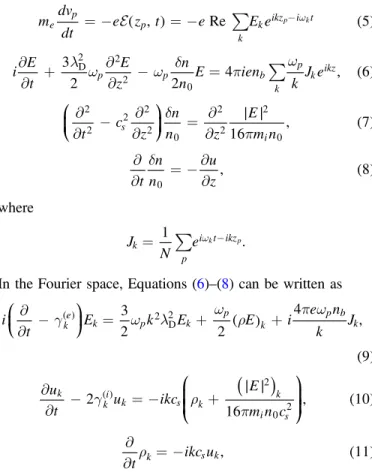
3.1. Langmuir Wave Decay in a Quasi-homogeneous Plasma Let usfirst consider simulations performed for a plasma with a small average level of densityfluctuations, i.e., Δn ; 0.001. Figure1shows the growth with time of the normalized spectral energy density WL=

å

by the beam and the corresponding time evolution of the beam velocity distribution f v( ); WL grows until saturation near

t 60000,

p

w  whereas f v( ) widens toward lower velocities, asymptoticallyforming a plateau with a vanishing slope

f v( ) v 0

¶ ¶  . Indeed, as Δn is verybelow the threshold

v v

3( T b)2

~ determined in our previous works (Krafft et al.

2013; Volokitin et al. 2013), the dynamics of the system

roughly presentsthe same features as those described by the quasilinear theory of the weak turbulence in homogeneous plasmas (Vedenov & Ryutov 1975, p. 3; see also Volokitin et al. 2013) or other close models (e.g., O’Neil et al. 1971; Volokitin & Krafft 2004; Krafft et al. 2005, 2010; Krafft & Volokitin2006, 2010; Zaslavsky et al. 2006, 2007; Krafft & Volokitin2013). In this case it was shown (e.g., Krafft et al. 2013) that the density inhomogeneities weakly influencethe

development of the beam instability and that the main features observed are (i) the formation of a plateau in the velocity distribution function f v( ) at asymptotic times, (ii) the dependence of the wave spectral energy density, scaling as

Ek2 nb n0 k k

4

(

)

( ) w

µ in the velocity domain above the

and(iii) a very small amount of accelerated beam electrons if Δn is not vanishing (e.g., Krafft et al.2013).

Up to the timew pt 30000,most features of the systemʼs evolution are in agreement with the predictions of the quasilinear theory of Langmuir waves. However, for

t 30000

p 

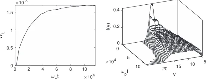
w , short-wavelength density oscillations, which have been identified as IS waves, appear and grow with time along the full length L of the system, as shown by Figure 2

which presents the Langmuir wave energy density E_{∣ ∣ and the}2

densityfluctuations n nd 0as a function of the space coordinate

z l at three different timesD w =pt 22000,28000, and 35000.

The short-wavelength density perturbations dnis n0 (see Equation (12)) present rather large amplitudes whereas the

Langmuir wave packets reveal energy densities E_{∣ ∣ peaking up}2 to around 0.01. To study thesefluctuations in more detailand separate them from the background long-wavelength fluctua-tions n nd 0, wefilter nd and the normalized plasma velocity u, which consists ofremoving all the Fourier harmonics nd k and

Figure 1. Left:time variation of the normalized spectral energy density WLof the Langmuir waves. Right:time variation of the beam velocity distribution f v( ); the

velocity v is normalized by vT. The main parameters are the following: nb n0= 105 -5, v vb T=14,D n 0.001,L=10000lD.

Figure 2. Left panels:profiles of the normalized wave energy density E_{∣ ∣}2 _{(turbulence parameter) at times t 22000,}

p

w = 28000, and 35000. Right panels:corresponding profiles of the density fluctuations n n0d ; short-scale oscillations are growing with time. The space coordinate z l ranges from 0 to theD size L of the simulation box. Parameters are the same as in Figure1.

uk with k<k_*~ – k2 3 b (kb=wp vb); we obtain the

short-wavelength density and plasma velocity in the form

nis n t e , u u t e . 12 k k k ikz is k k k ikz ( ) ( ) ( ) * *

å

å

Note that it is not essential to determine the exact value of k* and that we remove the parasitic oscillations thatremain after this operation at the edges of the chosen space portion where thefiltering is applied. Despite its arbitrariness, this procedure constitutes an effective method for analyzing the properties of the excited IS oscillations.

Using Equation(12), we present in Figure 3 the time and space variations of the turbulence parameter E_{∣ ∣ and the short-}2 scale oscillations dnis n over0 the full time range of the simulation. The dark lines traveling downward(Figure 3, left) correspond to Langmuir waves propagating along the beam direction with the group velocity v vg T 3kblD0.2 (kbl D 0.07). At wpt30000, IS waves appear (Figure 3,

right) thatpropagate in the beam direction with a velocity around the normalized IS velocity c vs T. Simultaneously (at

t 30000

p 

w ), Langmuir waves propagating in the direction opposite to the beam with the group velocity-v vg T-0.2 can be observed. This picture is in full agreement with the development of a nonlinear decay process during which a Langmuir wave  (wL,kL) transfers energy to a

counter-propagating Langmuir wave ¢ of frequency w_L¢ and wavenumber kL¢<0and an IS wave ¢(wS¢,kS¢>0). During

thisinteraction the conditions of parametric resonance w =L

L S

w ¢+w ¢ and kL= kL¢+kS¢ should be verified. As is well

known from the theory developed in homogeneous plasmas (Kadomtsev 1965; Nicholson & Goldman 1978), those are

satisfied if k_L¢k0-kL and kS¢2kL-k0, with kLkb

and k0l =D 2cs 3vT 0.03;corresponding wave dispersions

are L p 1 3kL 2

2 D 2

( )

w w + l and wS c k .s S¢ We show below

that in the present case these resonance conditions are fulfilled. Let us study the time evolution of the Langmuir and IS waves’ spectra. To distinguish between the IS waves propagating in the positive and the negative directions (i.e., in the direction of the beam propagation and opposite to it, respectively), we calculate the spectra of the Riemann invariants R+= +r u and R-=r-u, wherer=dn n0. In the absence of Langmuir waves, R+is conserved along the line

dz dt=cs for IS waves propagating in the positive direction

(increasing z in Figure 3) and R- is conserved along the line

dz dt= - for IS waves propagating in the negative directioncs

(decreasing z in Figure 3). Thus, the spectrum of the energy

density of the IS waves can be represented by S ,k with

Sk=[(r+u) ]2kfor k and S0 k=[(r-u) ]2kfor k< : S0 k

is the spectrum of the IS waves with k propagating in the0 positive direction and of the IS waves with k<0 propagating in the negative direction.

The spectra of the Langmuir and the IS waves’ energy densities Ek2 and Sk are calculated in Figure4 for the same

times as the profiles of E_{∣ ∣ and n n}2 0

d in Figure 2. The main peak centered near klDkblD0.07 in the Ek2 spectrum

corresponds to waves  excited by the beam instability near the most unstable mode aroundwk kvb- Dvb12.7vT

(Fig-ure 4, upper left); note that Ek2 broadens with time toward

higher kkb (i.e., lower phase velocities wk k<vb); no

waves with small k>0 are visible as wave scattering on the densityfluctuations nd is very weak. A second peak(waves ¢) appears atw pt 22000near klD-0.04; it grows with time, eventually reachingthe same amplitude as the other one at

kl D 0.07. Meanwhile, IS waves ¢ are excited around

kl D 0.11, as shown by the Sk spectrum at w pt 22000

(Figure4, lower left); this peak grows in correspondence with that at klD-0.04 (note that the peak near k = 0 in the Sk

spectrum corresponds to the initial density oscillations and should not beconsidered here). One can identify the first cascade of the decay process  ¢ + ¢. Indeed, the  theory of three-waves’ resonant decay in a homogeneous plasma predicts that for a parent Langmuir wave at

kLl D 0.07 we should get kL¢lD(k0-kL)lD-0.04 and kS¢lD(2kL-k0)lD 0.11, whichfits very well with the observations (Figure 4). Further (at wpt65000, not shown here), a second cascade of decay occurs, i.e.,

,

¢   +  providing Langmuir waves with k  LlD

kL 2k0 D 0.02

( - )l  and IS waves nearkSl =D

k k

2 L 3 0 D 0.05,

(- + )l - that propagate in the direction

opposite to the beam drift, i.e., with a group velocity-c vs T.

The secondary decay process is weaker than thefirst one and the amplitudes of the involved IS waves are smaller. Never-theless, the cascading process occurs two times, as expected by the theory(no further cascades as k kL 0<3); unless damping Figure 3. Left:space and time variations of the normalized Langmuir energy density E_{∣ ∣ . Right:}2 _{space and time variations of the corresponding short-scale density} fluctuations n nd is 0. Parameters are the same as in Figure1.

of waves is included (what is not the case here), there is no threshold for such decay processes.

The energy of the IS waves starts to grow when the Langmuir turbulence is almost saturated; thus, one can expect to observe a clear linear stage of the decay instability. Indeed, as shown in Figure5, the energy n n dz L

L is 0

2

ò

the short-scale IS oscillations(integrated over the full simula-tion box) grows exponentially within the time range

t

21000wp 37 000, whereas the corresponding Langmuir

energy E dz L

L 2 ∣ ∣

ò

n n dz L t 1 2 ln 2 3 10 , 13 p L is p 0 2 4 ( ) ( ) ⎛ ⎝ ⎜⎜

ò

which is indeed smaller than but close to the maximum growth rate of the decay instability given by Galeev et al. (1975) for

monochromatic waves in homogeneous plasmas

E n T 1 2 16 . 14 p S p e D 2 0 ∣ ∣ ( ) g w w w p 

Here wS is the frequency of the IS waves; then, as

c k

2 0.006

S p s b p

w w  w  and E∣ ∣2 16pn T0 e10-4 (aver-age value) we getg D 4 10-4wp. The uncertainty in the

determination of the average value of ∣ ∣E2 16pn T0 e in

Equation (14) and the fact that g_D is calculated for monochromatic waves in homogeneous plasmas can explain the difference betweenΓ and the theoretical value .g Note also_D that,as expected, the nonlinear growth rates Γ and g are_D

significantly smaller than the typical minimum frequency 0.006

S

w = of the wavesinvolved in the decay, ensuring that the collective response of the IS waves can take place as well as the exchanges of energy during the wave–wave coupling.

Finally, we can conclude that our simulations, which were carried out for a small average level Δn ; 0.001 of density fluctuations, are consistent with the theory of weak turbulence for Langmuir waves resonantly interactingwith IS waves through the channel  ¢ + ¢. Note that, obviously, the  beam instability does not excite a monochromatic wave but a broad wave spectrum. Then, as shown by the above figures, many waves of this wide packet can decay, producing a broad spectrum of daughter waves. The fastest Langmuir decay occurs for waves with the largestfield amplitudes, as shown by Figure 4. Upper panels:spectra Ek2of the Langmuir waves(in logarithmic scales) for the same instants of time as in Figure2, i.e.,w =pt 22000,28000, and 35000,

as a function of kl . Lower panels:Corresponding spectra (in logarithmic scales) of the energy density SD kof the IS waves with k0propagating in the positive

direction and of the IS waves with k<0propagating in the negative direction. Parameters are the same as in Figure1.

Figure 5. Time variation of the energy n n dz L

L is 0

2

ò d of the short-scale IS oscillations(thick line and left axis) and of the energy _{òL∣ ∣}E dz L2 _{of the} Langmuir waves(thin line and right axis)integrated over the full systemʼs length L, in logarithmic scales. Parameters are the same as in Figure1.

Equation(14), and the waves with larger k can undergo more

decay cascades than those with smaller k. After the occurrence of several cascades, the Langmuir energy can be accumulated within the region -k0 2 < <k k0 2, where waves cannot continue to decay but where the process of scattering off ions can become effective (see e.g., Cairns2000; Kontar & Pecseli

2002). However,this problem is not considered here.

The influence of the background density inhomogeneities on the systemʼs dynamics becomes significant only when Δn approaches or exceeds the threshold 3

(

)

our previous works (Krafft et al.2013; Volokitin et al.2013)

and the study we present hereinconcerning wave decay. We will consider in details successively two cases, when Δn = 0.01 and Δn = 0.02.

3.2. Langmuir Wave Decay in Inhomogeneous Plasmas with Random Density Fluctuations

When the average level of densityfluctuations Δn becomes of the order or larger than the threshold 3 vT vb

2

(

)

dynamics of the system isstrongly influenced by the scattering of the waves on the density inhomogeneities. Indeed, the wave–particle resonance conditions are violated due to the random variations of the waves’ phase velocities

k z k

k p( )

w w ; as a consequence, and compared to the homogeneous plasma case, the rate of growth of the Langmuir wave energy emitted during the bump-on-tail instability is decreased, while the relaxation time of the beam is increased. Moreover, due to their interactions with the density inhomo-geneities, Langmuir waves with larger k can transfer part of their energy to Langmuir waves with smaller k, which in turn can damp andaccelerate beam electrons of velocities

v>vb up to 2vb and more. Note also that in plasmas with

n 3 vT vb 2

(

)



D Langmuir waveforms tend to form spatially

localized and clumpy wave packets.

The presence of fluctuating density gradients generating various processes of wave reflection, refraction, and scattering as well as wave energy focusing alter the development of parametric instabilities occurring in plasmas with long-wavelength density inhomogeneities; some of the first reasons are, for example, the random variations of the wave frequencies and thus of the resonance conditions between waves,

k k k

w =w ¢+w , and the modification of the distribution of Langmuir wave energy in the k-space. Thus, the influence of

n 3 vT vb 2

(

)



D on the nonlinear dynamics of waves during

Langmuir turbulence is important, as revealed by the following simulation results.

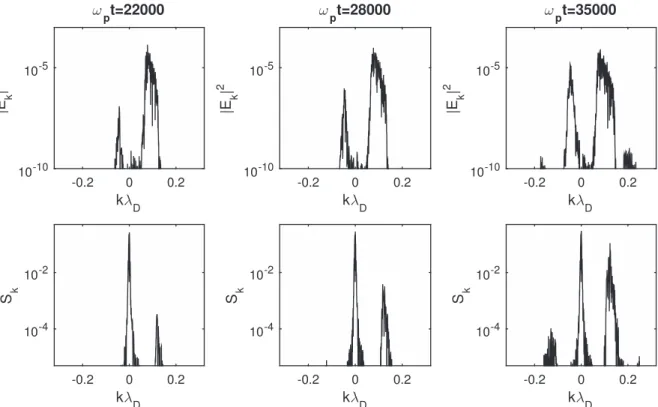
Figure 6 shows the time evolution of the Langmuir wave spectral energy WL and of the beam electron velocity

distribution f v( ) in a plasma with D n 0.01, near the threshold3

(

)

electrons (right panel) and the linked saturation of the wave energy growth(left panel, to compare with Figure1).

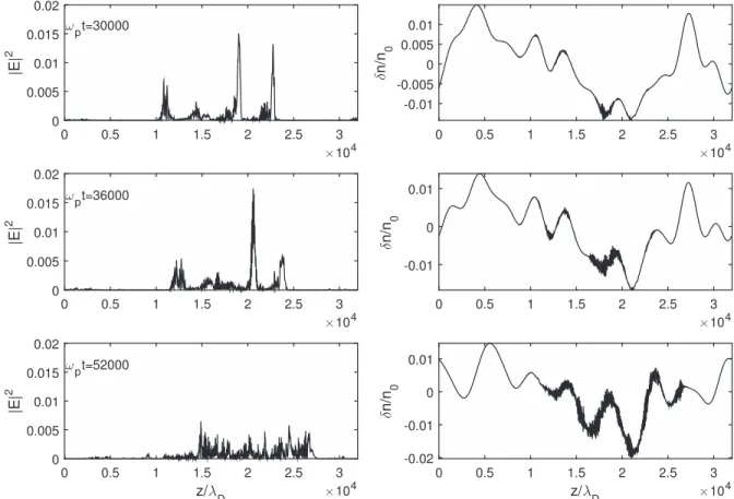
Profiles of the Langmuir wave energy E_{∣ ∣ and the density}2 fluctuations n nd 0 along the simulation box of length L are presented in Figure 7 for three different timesw =pt 30000, 36000, and 52000. One can see that Langmuir wave packets are focused and localized within a wide space region where the density fluctuations are forming a well (upper panels). Note that such observations were also done for density perturbations forming humps and not only depletions, as in the case presented here. After some time (middle panels) the local structure of the Langmuir waves, which form a set of more or less separated packets, is conserved despite the modification of the density profile. However, after the appearance of IS waves of noticeable intensity, the structure of the Langmuir packets becomes much more irregular and chaotic in the space region where short-scale density oscillations are rising(lower panels). This is due to the decay of Langmuir waves and to the consequent redistribution of energy between them, as shown below.

The spectra of the Langmuir and IS waves, shown in Figure 8 for the same times as in Figure 7, present features similar to those observed in Figure 4 for the case of small

n 0.001

D  ; indeed, one can observe peaks corresponding to the development of a decay instability. However, due to the presence of randomly varying density inhomogeneities, some differences exist between the theory of decay in quasi-homogeneous plasmas and the observations, as will be discussed below.

First, the wavenumber of the Langmuir mode observed near klD-0.05 at w pt 30000 and 36000 is consistent

with the value expected for a first decay cascade, i.e., Figure 6. Left:time variation of the normalized spectral energy density WLof the Langmuir waves. Right:time variation of the normalized beam velocity distribution

Figure 7. Left panels: profiles of the Langmuir wave energy E_{∣ ∣}2_{(turbulence parameter) at times t 30000,}

p

w = 36000, and 52000. Right panels:corresponding profiles of the density fluctuations n n .d 0 The space coordinate z l ranges from 0 to the size L of the simulation box. The parameters are the same as in FigureD 6.

Figure 8. Upper panels:spectra Ek2of the Langmuir waves, in logarithmic scales, for the same times as in Figure7. Lower panels:corresponding spectra (in

logarithmic scales) of the energy density Sk. The full ranges of space(box of length L=32000lD) and time of the system are considered (global spectra). The parameters are the same as in Figure6.

k_L¢lD(k0-kL)lD-0.06; the value of kL is determined

by the location of the highest peak with k> in the Langmuir0 spectrum at w pt 30000 (upper left panel, Figure 8), i.e.,

kLl D 0.09 (here k0l D 0.03 and kbl D 0.055; note that the most excited Langmuir waves have phase velocities

k v ,

k  b

w so that kL>kb). At the same time, the largest

peak in the IS spectrum is centered near kl D 0.15, which is very close to the expected wavenumber k_S¢lD

k k

2 L 0 D 0.15

( - )l  of IS waves produced during a first

decay cascade. Moreover, the peak at kl =D 0.025 in the Langmuir spectrum (upper left and middle panels) represents the mode kLlD=

(

)

k k

2 L 3 0 D 0.09

(- + )l - , which is close to the mode at

klD-0.1visible in the IS spectrum (lower middle panel). Let us stress that the complex peak structure in the low-frequency spectra can be attributed to the fact that several decay instability regions exist and interfere one with another. Moreover, effects due to Langmuir waves’ reflections on the density humps are essential and lead to the widening of the peaks in the corresponding wave spectra.

Second, one important difference compared to the quasi-homogeneous plasma case is that wave decay occurs in localized space-time regions. Indeed, for a given moment in the time range when decay occurs, there are not many occurrences of decay spread accross the full range of z (as in Figure3), but

the development of such a process can be observed only in two or three localized space regions. In this case, the processes of scattering, reflection, and/or 1D refraction modify the waves’ propagation locally, depending, for example, on the presence along the waves’ paths of more or less sharp gradients, deep wells, or wide humps, so that these waves can lose some part of their energy during their propagation, reducing by this fact the possibility of beingsubmitted to further decay processes along z. To understand how a locally arising nonlinear interaction of Langmuir waves with density fluctua-tions develops, let us focus our attention on finite portions

z z1, 2

[ ] of the simulation box. Figure 9 shows the

spatio-temporal evolution of the Langmuir wave energy E_{∣ ∣ and the}2 short-scale IS density fluctuations n nd is 0 in the subbox

z z1, 2 13000, 24000 D

[ ]=[ ]l , during the time interval

t

30000wp 54000. One can see the formation of three main regions of IS wave activity(right panel), which broaden and eventuallyintersect. Note the emergence of IS waves traveling in the direction opposite to the beam propagation with a group velocity around -c vs T, starting, for example, at

z21000lD and w pt 45000: they correspond to the

development of a second cascade of decay instability(see also above).

The left panel shows that the interactions of Langmuir packets with density fluctuations occur during limited and rather short time durations. Then, as their group velocity v vg T

significantlyexceeds the IS velocity c vs T, the Langmuir

waves can propagate away from these interaction regions; further, part of their energy can be transferred to Langmuir packets arising from a first decay cascade and propagating in the opposite direction, with a group velocity-v vg T (see,

for example, the wavescrossing near z21000lD and

t 47000

p

w  in the left panel). The beatings between Langmuir waves propagating in opposite directions lead to the generation of IS waves. Processes involving such beatings form a part of the cascade of energy transfer in the weak turbulence theory; however, some differences exist compared to the homogeneous plasma case: due to the presence of background density fluctuations, the decay processes are occurring locally, i.e., only in specific time and space regions. Figure10shows the“local” wave spectra corresponding to Figure 9, i.e., computed within a specific subbox [13000, 24000]l during a limited timeD 30000wpt54000. Those

reveal more clearly than the global ones—corresponding to the full space-time domain (Figure 8)—the development of a

cascade of energy transfer during the interaction of Langmuir and IS waves. This is particularly visible in the low-frequency spectra, with peaks appearing clearly in the vicinity of

kl =D 0.15 and -0.1. In the high-frequency spectra, peaks are excited near kl = -D 0.065,0.025, 0.065 and 0.09 (upper left panel); the largest one, which corresponds to beam-driven Figure 9. Space and time variations of E_{∣ ∣}2_{(left) and of the corresponding short-scale density fluctuations n n}

is 0

d (12) (right), in the limited area 13000, 24000[ ]lD and during the time interval30000<wpt<54000. The parameters are the same as in Figure6.

waves, is located at kl D 0.09. As discussed above, a first decay cascade of the Langmuir wave kLl D 0.09 starts, giving rise to a counterpropagating Langmuir wave at

k_L¢lD(k0-kL)lD -0.06 and to an IS wave with

kS¢lD=(2kL-k0)lD0.15. Further (at wpt30000),a

second decay cascade occurs, providing the peak at

kLlD=(kL-2k0)lD0.03 (upper right panel) and an IS wave atkSlD= -( 2kL+3k0)lD-0.09, propagating opposite to the beam. We obviously recover the same results as

above, but with significantly less ambiguity in the interpreta-tion of the spectral peaks.

Figure11shows the profiles of the Langmuir wave energy

E 2

∣ ∣ and the densityfluctuations n nd 0within the same spatio-temporal area as in Figures 9–10. IS waves’ short-scale oscillations appear first at w =pt 35000 within the region

z

17000lD< <20000lD; further they extend over wider space domains, eventuallyoccupyingfor wpt50000 the subarea 13000, 24000[ ]l . However, they do not extend overD Figure 10. Upper panels:“local” spectra Ek2of the Langmuir waves, in logarithmic scales, for the same times as in Figures7and8. Lower panels:corresponding

“local” spectra (in logarithmic scales) of the energy density Sk. All spectra are computed in the limited space-time area corresponding to 13000, 24000[ ]lDand

t

30000<wp <54000. The parameters are the same as in Figure6.

Figure 11. Profiles of the normalized Langmuir wave energy density E_{∣ ∣}2_{(right axis and lower curves in each panel) superposed to the density fluctuations n n0d (left} axis and upper curves), in the area 13000 , 24000[ lD l , at timesD] w =pt 35000,40000, 45000, and 50000. Note that the origin of both vertical axes are not coinciding.

the whole space profile (see also Figure7). One can observe

that the various space regions of IS waves’ generation are separated one from the other. Moreover, in each area where these waves appear, the growth of their energy stops when the Langmuir packets have traveled away and left the interaction region due to the large difference between the IS and the Langmuir waves’ group velocities, vgcs (compare, for

example, the panels at w =pt 35000 and w =pt 40000). The

escaping Langmuir waves can then interact with IS waves in other space-time regions where such oscillations appear.

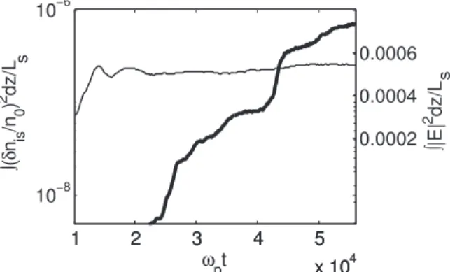
Figure12 shows the time variation of the IS and Langmuir waves’ energies, n n dz L L is 0 s 2 s

ò

ò

respec-tively, obtained by simulations involving a plasma with density fluctuations of larger average level, i.e., D n 0.02 (other parameters being the same as in Figure1) and computed in the

limited domain Ls=[13000lD, 24000lD]. One can see that, whilethe plasma waves’ energy varies only slightly, the energy of the IS short-scale oscillations nd is n0exhibits two periods of exponential growth; each of them corresponds to the growth of a localized IS wave packet rising in a specific region of the subbox Ls. The first period, between wp( )t 24000 and

t 28000,

p

w  corresponds to the crossing of two Langmuir packets of positive but different group velocities; indeed, when a Langmuir packet passes through a density hump, its group velocity can be significantly reduced due to 1D refraction effects. The second period, i.e., 42000wpt 46000 (see also Figure9), corresponds to the occurrence of a first cascade

of Langmuir waves’ decay, whose growth rate can be estimated as G =2.7 10-4wp (with g D 4 10-4wp,;see

Equa-tions(13)–(14)).

Let us present in this case a typical example of Langmuir decay involving several cascades. Figure13shows the spatio-temporal variation of the Langmuir wave energy density E_{∣ ∣}2 and of the short-scale density oscillations nd is n0, in the subbox

5000, 8000 D

[ ]l and the time interval 4500wpt9000, when the beam instability is saturated. In the left panel, beam-driven Langmuir waves are propagating with vg>0 through the region 5000, 6700[ ]l forD wpt58000; nearw pt 58300

and z6800lD,their amplitudes are strongly enhanced when they cross another Langmuir packet traveling with vg < . At0 the same time, IS waves propagating with the group velocity

c vs T >0 are excited(right panel).

In Figure14, which shows the corresponding profiles of E_{∣ ∣}2 and n nd 0(including n nd is 0) at six moments of time, one can see that E_{∣ ∣ reaches its maximum when the waves approach}2 the local density hump near z6800lD(left middle panel at

t 58300

p

w  ); at this point,both packets propagating in opposite directions interact and, as a result, some large part of the Langmuir energy is reflected and propagates away with

vg<0 (see Figure 13, left, and Figure 14, top right). A similar event can be observed later, near w pt 60000 and

z7300lD (Figure 13, left): the Langmuir wave decays. Figure 14 at wp( )t 60600 and 63000 shows how the counterpropagating packet separates itself from the packet with vg> , eventually takingwith it almost all the0 Langmuir energy. The two peaks atw pt 63000 (Figure 14 , bottom right) can be clearly identified in Figure 13 as the two packets propagating with vg< , in the time range0

t

60000 wp 65000. Moreover, near w pt 66000 and

z6000lD, a second decay cascade occurs, giving rise to Langmuir packets propagating with vg>0 and IS waves’ oscillations propagating with-c vs T <0 (Figure13).

It is well known from theory(Musher et al.1995) that decay

processes involve several cascades of energy transfer to waves with longer wavelengths. The successive occurrence of two decay cascades was discussed and presented above for the cases of very small orfinite average levels of external density fluctuations, i.e., for Δn ; 0.001 and Δn ; 0.01 (see, e.g., Figure10). However, one muststress that decay cascading in a

plasma with background density fluctuations of finite Δn presents specific features, whichwe examine now in more detailon the basis of simulation results presented in Figures12–14. Notefirst thataccording to the decay resonance conditions, only three cascades are expected to occur for the beam and plasma parameters considered here. During these successive processes, Langmuir wavenumbers decrease more and more, starting from the value kLl D 0.11corresponding to the most excited beam-driven Langmuir waves (not shown here); then, as a consequence of the resonance conditions, the Langmuir wave products of thefirst, second, and third decay cascades are characterized by the following wavenumbers: k_L¢lD

k0 kL D 0.08,

( - )l - kLlD(kL-2k0)lD0.05, and

kL‴lD(3k0-kL)lD-0.02, whereas for the IS daughter waves we have kS¢lD(2kL-k0)lD0.19, kSlD

k k

2 L 3 0 D 0.13

(- + )l - , and kS‴lD(2kL-5k0)lD 0.07, respectively. A fourth cascade is not possible as the resonance conditions are not fulfilled. An essential point lies in the fact that the Langmuir waves  coming from the second cascade propagate in the direction of the beam drift and have larger phase velocities than those excited first by the beam instability. So the second decay cascade can play an important role in the acceleration of beam electrons above the initial beam velocity vb.

The first two decay cascades are very clearly observed in Figures 13–14. Forwpt56000 and z6800l , two waveD packets propagate along the beam direction(vg> ) and a third0 one in the opposite direction (vg< ) (Figure0 13, left). In the vicinity of z6900lD, the packet with vg>0 and with the

largest amplitude collides near w pt 58000 with the packet propagating with vg<0 (see also Figure14atw pt 58300).

IS waves are generated as a result of the beating between these two colliding packets(Figure13, right); during this process, the weaker amplitude packet with vg<0 gets energy from the more intense one with vg> . This mechanism could be0 Figure 12. Time variations of the energy densities of the IS short-scale

oscillations(bold line, left axis) and of the Langmuir waves (thin line, right axis), i.e., n n dz L L is 0 2 s ò d and E dz L L 2 s∣ ∣ ò , respectively, in logarithmic scales; the energies are computed within a localized area Lsof the simulation

box, in the range15000wpt55000. The main parameters are the following: nb n0= 105 -5, v vb T=14,D n 0.02,L=10000lD.

considered as thefirst cascade of wave energy transformation, but the actual situation is more complicated. Indeed, almost simultaneously, the colliding packet with vg > reflects on the0 density hump presenting a maximum at z7000lD(Figure14 atw pt 58300). The propagatingsecond packet with vg>0

consequently collides with the amplified packet with vg<0 and with the reflected one (Figure 13, left;Figure 14 at

t 59300

p

w  ). Their beatings also generate IS waves. At

t 60000

p 

w two wave packets are traveling in the direction opposite to the beam propagation (Figure14atw pt 63000). Later, near w pt 67000 and z6000lD, a process starts

which can be called the second decay cascade, involving one of these packets and generating IS waves propagating in the negative direction (at group velocity c v- s T)with no

signa-tures of any Langmuir wave reflection (Figure 13, left). At last, near ( tw p 73500, z6800lD) and ( tw p 76000,

z7800lD), structures similar to a third decay can be observed on the space-time evolution pattern(Figure 13, left); one can indeed observe a small but noticeable enhancement of the IS wave emission along the direction of the beam propagation, near w pt 73500 and z6800lD (Figure 13, right), which is expected from a third cascade; however, as the Figure 13. Space and time variations of E_{∣ ∣}2_{(left) and of the corresponding short-scale density fluctuations n n}

is 0

d (right), in the area 5000, 8000[ ]l . The parametersD are the same as in Figure12.

Figure 14. Profiles of the Langmuir wave energy density E_{∣ ∣}2_{(right axis and lower curves in each panel) superposed to the density fluctuations n n0d (left axis and} upper curves), in the area 13000 , 24000[ lD l , at timesD] w =pt 57000,58300, 59300, 59600, 60600, and 63000. Note that the zero of both vertical axes are not

wave packets haveamplitudes that are too weak, we are not able to state that this process is actually and certainly a third cascade. Indeed, Figure 15 presents the corresponding local spectra of Langmuir and IS waves at the three time moments

t 62000,

p

w = 68000, and 74000; they show thatif peaks at

kL‴lD-0.02 (upper right panel) and kS‴l D 0.07 (lower right panel) are visible, they are either too weak (IS spectrum) or mixed with other effects (Langmuir spectrum). However, at

t 62000

p

w = andw =pt 68000, the position of some peaks in the IS and Langmuir spectra are very close to those predicted by the resonant wave decay theory in homogeneous plasmas for thefirst and the second cascades (see the discussion in the previous paragraph). As mentioned above, the spectrum of Langmuir waves for w =pt 74000 does not show clearly distinguishable peaks, whichcan be explained by two effects, i.e., the propagation of the waves in the inhomogeneous plasma and their exchanges of energy with the beam. At the same time, three main peaks can be observed in the IS spectrum: two correspond to the wavenumbers of the IS wave products of the twofirst decay cascades, i.e., kS¢lD0.19and

kSlD-0.13, whereas the third one near klD-0.2 is likely due to a nonresonant wave–wave interaction.

Finally, it is important to stress at this stage that it is generally very difficult, if not impossible, to separatethe processes of wave reflection on density fluctuations from that ofparametric wave–wave interactions; both effects are usually working together in a inhomogeneous plasma, and the origin of the counterpropagating (i.e., with vg< ) Langmuir waves0 produced cannot be determined conclusivelyin most cases. Note also that reflections of Langmuir waves on long-wavelength density inhomogeneities can, in some conditions, favor the emergence of nonlinear decay processes, owing to the

appearance of parametric interaction processes involving waves traveling in the direction opposite to the beam propagation. One must alsotake into account the significant role of the variations of the long-wavelength density fluctuations due to their own dynamics; for example, the local positive gradient of the density hump in Figure14disappears forwpt 63000and conditions for IS wave generation in the vicinity of this region become less favorable than when Langmuir energy can focus on the gradients of the humps near some reflection points.

4. DISCUSSION AND CONCLUSION

Simulations have shown that three-wave decay processes including several cascades can occur in inhomogeneous plasmas as those of the solar wind in the source regions of type III bursts and, in particular, in the course of Langmuir turbulence in the presence of electron beams. Wave–wave interaction processes where a Langmuir wave decays into a Langmuir and whereIS waves can be observed in plasmas with average levels of density fluctuations up to a few percent. Decay has been notably identified by the simultaneous presence of peaks in the high- and low-frequency wave energy spectra, at the wavenumbers of the mother and the daughter waves, in agreement with the waves’ resonance conditions. Moreover, the growth rate of the IS energy has been shown to fit with the predictions of the parametric decay theory for homogeneous plasmas and monochromatic waves, at least up toΔn ; 0.02. A very good agreement between the wavenum-bers predicted by this theory and our simulations of Langmuir turbulence in inhomogeneous plasmas has been observed. This is due to the fact that the waves’ dispersion equations are not significantly modified by the irregularities and that the Figure 15. Local spectra (computed in the area 4500, 8500[ ]lD) of Langmuir and ion sound waves for three moments of timew =pt 62000,68000, and 74000. The