Emulating IPCC AR4 atmosphere-ocean and carbon cycle models for projecting global-mean, hemispheric and land/ocean temperatures: MAGICC 6.0

HAL Id: hal-00304059

https://hal.archives-ouvertes.fr/hal-00304059

HAL is a multi-disciplinary open access

archive for the deposit and dissemination of sci-entific research documents, whether they are pub-lished or not. The documents may come from teaching and research institutions in France or abroad, or from public or private research centers.

L’archive ouverte pluridisciplinaire HAL, est destinée au dépôt et à la diffusion de documents scientifiques de niveau recherche, publiés ou non, émanant des établissements d’enseignement et de recherche français ou étrangers, des laboratoires publics ou privés.

Emulating IPCC AR4 atmosphere-ocean and carbon

cycle models for projecting global-mean, hemispheric

and land/ocean temperatures: MAGICC 6.0

M. Meinshausen, S. C. B. Raper, T. M. L. Wigley

To cite this version:

M. Meinshausen, S. C. B. Raper, T. M. L. Wigley. Emulating IPCC AR4 atmosphere-ocean and carbon cycle models for projecting global-mean, hemispheric and land/ocean temperatures: MAGICC 6.0. Atmospheric Chemistry and Physics Discussions, European Geosciences Union, 2008, 8 (2), pp.6153-6272. �hal-00304059�

ACPD

Full Screen / Esc

Printer-friendly Version Interactive Discussion Atmos. Chem. Phys. Discuss., 8, 6153–6272, 2008

www.atmos-chem-phys-discuss.net/8/6153/2008/ © Author(s) 2008. This work is distributed under the Creative Commons Attribution 3.0 License.

Atmospheric Chemistry and Physics Discussions

Emulating IPCC AR4 atmosphere-ocean

and carbon cycle models for projecting

global-mean, hemispheric and land/ocean

temperatures: MAGICC 6.0

M. Meinshausen1, S. C. B. Raper2, and T. M. L. Wigley3

1

Potsdam Institute for Climate Impact Research (PIK), Potsdam, Germany 2

Manchester Metropolitan University (MMU), Manchester, UK 3

National Center for Atmospheric Research (NCAR), Boulder, CO, USA

Received: 20 December 2007 – Accepted: 6 January 2008 – Published: 27 March 2008 Correspondence to: M. Meinshausen (malte.meinshausen@pik-potsdam.de)

ACPD

Full Screen / Esc

Printer-friendly Version Interactive Discussion

Abstract

Current scientific knowledge on the future response of the climate system to human-induced perturbations is comprehensively captured by various model intercomparison efforts. In the preparation of the Fourth Assessment Report (AR4) of the Intergov-ernmental Panel on Climate Change (IPCC), intercomparisons were organized for 5

atmosphere-ocean general circulation models (AOGCMs) and carbon cycle models, named “CMIP3” and “C4MIP”, respectively. Despite their tremendous value for the sci-entific community and policy makers alike, there are some difficulties in interpreting the results. For example, key radiative forcings have not been considered or standard-ized in the majority of AOGCMs integrations and carbon cycle runs. Furthermore, the 10

AOGCM analysis of plausible emission pathways was restricted to only three SRES scenarios. This study attempts to address these issues. We present an updated version of MAGICC, the simple carbon cycle-climate model used in past IPCC As-sessment Reports with enhanced representation of time-varying climate sensitivities, carbon cycle feedbacks, aerosol forcings and ocean heat uptake characteristics. This 15

new version of MAGICC (6.0) is successfully calibrated against the higher complexity AOGCM and carbon cycle models. Parameterizations of MAGICC 6.0 are provided. Previous MAGICC versions and emulations shown in IPCC AR4 (WG1, Fig. 10.26, page 803) yielded, in average, a 10% larger global-mean temperature increase over the 21st century compared to the AOGCMs. The reasons for this difference are dis-20

cussed. The emulations presented here using MAGICC 6.0 match the mean AOGCM responses to within 2.2% for the SRES scenarios. This enhanced emulation skill is due to: the comparison on a “like-with-like” basis using AOGCM-specific subsets of forc-ings, a new calibration procedure, as well as the fact that the updated simple climate model can now successfully emulate some of the climate-state dependent effective 25

climate sensitivities of AOGCMs. The mean diagnosed effective climate sensitivities of the AOGCMs is 2.88◦C, about 0.33◦C cooler than the reported slab ocean climate sensitivities. Finally, we examine the combined climate system and carbon cycle

em-ACPD

Full Screen / Esc

Printer-friendly Version Interactive Discussion ulations for the complete range of IPCC SRES emission scenarios and some lower

mitigation pathways.

1 Introduction: the value of simple climate models

Since the introduction of three-dimensional coupled atmosphere-ocean general circu-lation models (AOGCMs) (e.g.Manabe and Bryan,1969;Manabe et al.,1975;Bryan

5

et al.,1975), one goal of Earth system science for understanding the past and pro-jecting the future is to build highly resolved, comprehensive and coupled models of the physical atmosphere and ocean dynamics, including models of the Earth’s cryosphere, terrestrial and marine biota. Depending on the research question, though, intermedi-ate complexity or simpler models will remain more suitable research tools, due to their 10

focus on individual processes, their ability to encompass part of the structural uncer-tainties of complex models, and/or their computational efficiency. After the introduction of the one-dimensional upwelling-diffusive ocean model byHoffert et al.(1980), early applications of simple models were able to give insights into climate system behaviour as their relative simplicity allowed isolation and investigation of individual feedback pro-15

cesses, multi-thousand year simulations, and various parameterizations (Harvey and

Schneider,1985b,a;Hoffert et al.,1980;Schneider and Thompson,1981). Recently, this role has also been filled by intermediate complexity models. Shifting from their role as models in their own right, simple models started to serve four distinct purposes as exemplified in this study:

20

I) Emulations. Simple models are used to emulate global or large-scale averaged

quantities of AOGCMs (see e.g.Schlesinger and Jiang,1990,1991). In most cases, AOGCMs are still computationally too expensive for large ensembles for different emis-sion scenarios and/or perturbed physics experiments except in special circumstances (Allen, 1999;Stainforth et al., 2005). A precondition for the quantitative reliability of 25

AOGCM emulations is that the emulation of the variables of interest is suitably accu-rate over a wide range of scenarios actually performed with AOGCMs. Various authors

ACPD

Full Screen / Esc

Printer-friendly Version Interactive Discussion (e.g.Raper and Cubasch,1996;Kattenberg et al.,1996;Raper et al.,2001;Cubasch

et al.,2001;Osborn et al.,2006) have shown for example that the upwelling-diffusion model MAGICC, the primary simple climate model used in past IPCC Assessment Re-ports, can closely match key large-scale AOGCMs results.

In the preparation of the Intergovernmental Panel on Climate Change Fourth Assess-5

ment Report (IPCC AR4), fourteen modeling groups submitted data for 23 AOGCMs, building the World Climate Research Programme’s (WCRP’s) Coupled Model Inter-comparison Project phase 3 (CMIP3) multi-model dataset. Each of these AOGCMs is structurally different (although the degree to which they differ is variable), leading to variations in their climate response characteristics. In the present study we show 10

emulations of oceanic heat uptake and surface air temperatures over land and ocean in both hemispheres for 19 of these AOGCMs (i.e., those for which suitable data were available). In addition to the no-climate-policy SRES scenarios analyzed in IPCC AR4, we also present joint AOGCM and carbon cycle model projections for a set of multi-gas mitigation scenarios and pathways.

15

II) Spanning structural uncertainties. The advantage of simple models is that

struc-tural uncertainties across a large set of complex models can be captured. Strucstruc-tural uncertainties are reflected by the different choices made by modeling groups, e.g. what key processes should be included and how they should be modeled. Parametric un-certainty, in contrast, is the uncertainty arising from choices in the parameter values 20

for a model with given structure. In practice, a strict separation between these two types of uncertainties is not possible. In fact, we take advantage of this overlap in the present study by “parameterizing” the structural uncertainty range of more com-plex models (cf.O’Neill and Melnikov,2008). This approach is distinct from perturbed physics studies with intermediate complexity models or AOGCMs, which often concen-25

trate on assessing parametric uncertainties. Sufficiently flexible simple models, once calibrated to sophisticated models help to indicate structural uncertainties, for a lim-ited set of key quantities, like hemispheric mean temperatures and only to the extent that variations in the AOGCM responses are due to structurally different model

com-ACPD

Full Screen / Esc

Printer-friendly Version Interactive Discussion ponents. As shown in this study, calibrating a simple model to the CMIP3 AOGCMs

provides some measure of structural uncertainty, e.g. in regard to the models’ feedback processes summarized by the calibrated climate sensitivity parameter. This structural uncertainty can then be translated to scenarios, which were not run by all AOGCMs.

III) Factor separation analysis. Simple models can assist in factor separation

anal-5

ysis, i.e., separating climate or carbon cycle responses from forcing uncertainties or investigating the effects due to different initialization choices. Thus, simple models can assist in harmonizing AOGCM and other higher complexity model responses, e.g. by estimating their responses for unified forcing assumptions. A major difficulty in inter-preting the multi-model AOGCM projections presented in IPCC AR4 arises from the 10

different sets of radiative forcings agents considered by the various modeling groups (see Table 10.1 inMeehl et al.,2007). Even for the common forcings, the magnitude and time-evolution differs from model to model for the same scenario. For example, some models applied only very weak volcanic forcing in the 20th century runs, while some ignored volcanic forcing completely; some models varied tropospheric ozone, 15

while others kept the forcing by tropospheric ozone constant for the 21st century. Further complications arise due to the fact that for most AOGCMs, the forcing time-series are not diagnosed or documented from the model runs – with some exceptions likeTakemura et al.(2006) andHansen et al.(2005). Different reporting standards for radiative forcing, like reporting adjusted forcing after thermal stratospheric adjustment 20

at the model’s tropopause or at 200 hPa level, further hinder comparability, even if some diagnostic data are provided as for the doubled CO2 concentration experiments (see

e.g. Table 2 inForster and Taylor,2006). In addition, studies comparing the radiative transfer schemes in AOGCMs found surprisingly large differences from the line-by-line code, even for well known forcing agents like CO2 (Collins et al.,2006). In summary,

25

imperfect knowledge with regard to the forcings in CMIP3 AOGCMs leads to ambigu-ities as to whether differences in their climate responses are due to different climate responses or partly an expression of different (sometimes limited or erroneous) radia-tive forcing implementations.

ACPD

Full Screen / Esc

Printer-friendly Version Interactive Discussion Faced with these challenges, this study attempts to separate radiative forcing and

climate response uncertainties in AOGCMs. Thus, using “like-with-like” forcing time series to match the AOGCM specific sets of considered forcing agents, the parame-terizations in the simple climate model are calibrated to match the AOGCMs’ climate responses. Subsequent emulations take into account the complete set of key forc-5

ing agents – thereby providing an estimate of the AOGCMs’ response had all major forcings been considered.

IV) Joint response and feedback analysis. Simple, but sufficiently comprehensive,

models allow estimating the coupled responses of multiple models of higher complexity. One example are the uncertainties in radiative forcing of well-mixed greenhouse gases, 10

which are to some degree independent from the climate response to the forcing. A simple model could combine forcing and climate response uncertainties by emulating all permutations of AOGCM climate response characteristics and respective radiative transfer scheme results.

Another example relates to the fact that many of the AOGCMs used in the IPCC 15

AR4 were not yet coupled to an interactive carbon cycle and so had to be driven with externally calculated CO₂concentrations. Thus, in most cases the same CO₂ concen-trations were prescribed for a “warmer” and a “colder” AOGCM, despite the fact that the warmer AOGCM is likely to see higher concentrations under the same emission sce-nario. MAGICC is a coupled gas-cycle/climate model and, as such, includes feedbacks 20

between the carbon cycle and the climate. Hence, for any set of model parameters, MAGICC is internally consistent in that the climate feedbacks on the CO2 projections

will be driven by the climate model output.

This study combines a full range of AOGCM emulations with emulations of the most complete set of carbon cycle models to date (C4MIP,Friedlingstein et al.,2006). Ten of 25

the eleven C4MIP carbon cycle models and their terrestrial and oceanic carbon pools and fluxes are emulated. For the first time, a large set of both carbon cycle and climate models has been emulated individually. This allows a sizeable combined ensemble for each emission scenario with 190 combinations of nineteen emulated AOGCM climate

ACPD

Full Screen / Esc

Printer-friendly Version Interactive Discussion and ten C4MIP carbon cycle responses, providing a better estimate of uncertainties in

the climate projections than would otherwise be possible.

This study presents the most comprehensive AOGCM and carbon cycle model em-ulation exercise to date. We use an updated version of MAGICC, which was origi-nally developed byWigley and Raper(1987,1992) and amended continuously since 5

then (see e.g.Raper et al.,1996;Wigley and Raper,2001). Several amendments to MAGICC have been spurred by new results presented in IPCC AR4 as well as the increasing availability of comprehensive AOGCM and C4MIP datasets. For example, land/ocean hemispheric temperature evolutions of both hemispheres were calculated for each AOGCM allowing for a more in-depth analysis of optimal heat exchange pa-10

rameterizations in MAGICC. Of course, emulations with a simple model like MAGICC 6.0 can by no means replace research into more sophisticated carbon cycle and gen-eral circulation models. Rather, what MAGICC 6.0 offers is primarily a method to ex-tend the knowledge created with AOGCMs and carbon cycle model runs in order to provide estimates of their joint responses and to extrapolate their key characteristics 15

to a range of other scenarios. This study is partially motivated by the MAGICC 4.2 emulation results presented in IPCC AR4, which showed in average an about 10% warmer response over the period from 1990 to the end of the 21st century for the SRES scenarios, despite closely matching the idealized CO2-only scenarios.

This paper is structured as follows: Sect. 2 provides a brief overview of the main 20

amendments in the climate model MAGICC 6.0 as used here – compared to the ver-sion used in IPCC AR4. The calibration procedures and forcing harmonization for emulating CMIP3 AOGCMs and C4MIP carbon cycle models are described in Sect.3. The emulation results as well as the effects of the forcing adjustments are provided in Sect. 4. Section 5 discusses the present calibration results, particularly in regard to 25

diagnosed climate sensitivities. In addition, Sect.5provides an analysis of calibrations to AOGCM with a previous version of MAGICC, as presented in IPCC AR4. Climate responses to a large set of non-mitigation and mitigation scenarios are provided in Sect.6. Section7summarizes limitations of the present approach, while conclusions

ACPD

Full Screen / Esc

Printer-friendly Version Interactive Discussion are given in Sect.8. A complete description of the MAGICC 6.0 model can be found in

AppendixA.

2 Model description

MAGICC has a hemispherically averaged upwelling-diffusion ocean coupled to an at-mosphere layer and a globally averaged carbon cycle model. As with most other simple 5

models, MAGICC evolved from a simple global average energy-balance equation. This energy balance equation of the perturbed climate system can be written as:

Q_G= λG∆TG+

d H

d t (1)

whereQ_G is the global-mean radiative forcing at the top of the troposphere. This ex-tra energy influx is partitioned into increased outgoing energy flux and heat content 10

changes in the ocean d H_{d t}. The outgoing energy flux is dependent on the global-mean feedback factor,λ_G, and the surface temperature perturbation ∆TG.

While MAGICC is designed to provide maximum flexibility in order to match differ-ent types of responses seen in more sophisticated models, the approach in MAGICC’s model development has always been to derive the simple equations as much as possi-15

ble from key physical and biological processes. In other words, as simple as possible, as mechanistic as necessary. This process-based approach might be an advantage in comparison to simple statistical fits that are more likely to quickly degrade in their skill when emulating scenarios outside the original calibration space of sophisticated models.

20

The main improvements in MAGICC 6.0 compared to the version used in the IPCC AR4 are briefly highlighted in this section. The options introduced to account for vari-able climate sensitivities are described (Sect.2.1). With the exception of the updated carbon cycle routines (Sect. 2.2), the new parameterizations encompass the IPCC AR4 MAGICC parameterizations as a special case, i.e., the IPCC AR4 version can be 25

ACPD

Full Screen / Esc

Printer-friendly Version Interactive Discussion 2.1 Introduction of variable climate sensitivities

Climate sensitivity (∆T2x) is a useful metric to compare models and is usually defined

as the global-mean equilibrium warming after a doubling of CO₂ concentrations (from pre-industrial levels). Climate sensitivity is inversely related to the feedback factorλ:

∆T2x =

∆Q2x

λ (2)

5

where ∆T2x is the climate sensitivity, and ∆Q2x the radiative forcing after a doubling of

CO2concentrations (see energy balance Eq.A46).

The (time- or state-dependent) effective climate sensitivity (St) (Murphy and Mitchell,

1995) is defined using the transient energy balance Eq. (1) and can be diagnosed from model output for any part of a model run where radiative forcing and ocean heat uptake 10

are both known and their sum is different from zero, so that:

St= ∆Q2x λt = ∆Q2x× ∆TGLt Qt₋d H d t|t (3)

where ∆Q2x is the model-specific forcing for doubled CO2 concentration, λt is the

time-variable feedback factor,Qt the radiative forcing, ∆TGLt the global-mean

temper-ature perturbation and d H_{d t}|t the climate system’s heat uptake at time t. By definition, 15

the traditional (equilibrium) climate sensitivity (∆T2x) is equal to the effective climate

sensitivityStat equilibrium (d H_{d t}|t=0) after doubled (pre-industrial) CO2concentration.

If there were only one globally homogenous, fast and constant feedback process, the diagnosed effective climate sensitivity would always equal the equilibrium climate sensitivity ∆T2x. However, many CMIP3 AOGCMs exhibit variable effective climate

sen-20

sitivities, often increasing over time (e.g. models CCSM3, CNRM-CM3, GFDL-CM2.0, GFDL-CM2.1, GISS-EH – see Figs. 16, 17, and 18). This is consistent with earlier results of increasing effective sensitivities found bySenior and Mitchell (2000);Raper

ACPD

Full Screen / Esc

Printer-friendly Version Interactive Discussion higher sensitivities for higher forcing scenarios (1pctto4x) than for lower forcing

sce-narios (1pctto2x) (e.g. ECHAM5/MPI-OM and GISS-ER, see Fig.1).

In order to better emulate these time-variable effective climate sensitivities, this ver-sion of MAGICC incorporates two modifications: Firstly, an amended land-ocean heat exchange formulation allows effective climate sensitivities to increase on the path to 5

equilibrium. In this formulation, changes in effective climate sensitivity arise from a geometrical effect: spatially non-homogenous feedbacks can lead to a time-variable effective global-mean climate sensitivity, if the spatial warming distributions change over time. Hence, by modifying land-ocean heat exchange in MAGICC, the spatial evo-lution of warming is altered, leading to changes in effective climate sensitivities given 10

that MAGICC has different equilibrium sensitivities over land and ocean (Raper,2004). Secondly, the climate sensitivity, and hence the feedback parameters, can be made explicitly dependent on the current forcing at time t. Both amendments are detailed in the AppendixA(see Sects. A4.2and A4.3). Although these two amendments both modify the same diagnostic, i.e., the time-variable effective sensitivities in MAGICC, 15

they are distinct: the land-ocean heat exchange modification changes the shape of the effective climate sensitivity’s time evolution to equilibrium, but keeps the equilibrium sensitivity unaffected. In contrast, making the sensitivity explicitly dependent on the forcing primarily affects the equilibrium sensitivity value.

Note that time-varying effective sensitivities are not only empirically observed in 20

AOGCMs, but they are necessary here in order for MAGICC to accurately emulate AOGCM results. Even with a constant (best-fit) sensitivity, however, MAGICC is able to provide good (but less than optimal) fits to these more sophisticated models.

Alternative parameterizations to emulate time-variable climate sensitivities are pos-sible, e.g. assuming a dependence on temperatures instead of forcing. However, this 25

study chose to limit the degrees of freedom in respect to time-variable climate sen-sitivities given that a clear separation into three (or more) different parameterizations seemed speculative based on the AOGCM data analyzed here. Further studies like the recent ones byAndrews and Forster(2008) orGregory and Webb(2008) on

semi-ACPD

Full Screen / Esc

Printer-friendly Version Interactive Discussion direct forcings or instantaneous, fast and longer term adjustment effects to various

forcings will help to refine the optimal parameterizations to emulate AOGCMs in the future.

2.2 Updated carbon cycle

MAGICC’s terrestrial carbon cycle model is a globally integrated box model, similar to 5

that in Harvey (1989) and Wigley (1993). The MAGICC 6.0 carbon cycle can emu-late temperature-feedback effects on the heterotrophic respiration carbon fluxes. One improvement in MAGICC 6.0 allows increased flexibility when accounting for CO2

fer-tilization. This increase in flexibility allows a better fit to some of the more complex carbon cycle models reviewed in C4MIP (Friedlingstein et al.,2006) (see Sect.3.3). 10

Another update in MAGICC 6.0 relates to the relaxation in carbon pools after a defor-estation event. The gross CO₂ emissions related to deforestation and other land use activities are subtracted from the plant, detritus and soil carbon pools (see Fig. 13). While in previous versions only the regrowth in the plant carbon pool was taken into account to calculate the net deforestation, MAGICC 6.0 includes now an effective re-15

laxation/regrowth term for all three terrestrial carbon pools (see AppendixA1.1). The original ocean carbon cycle model used a convolution representation Wigley

(1991b) to quantify the ocean-atmosphere CO₂flux. A similar representation is used here, but modified to account for nonlinearities. Specifically, the impulse response representation of the Princeton 3-D GFDL model (Sarmiento et al., 1992) is used to 20

approximate the inorganic carbon perturbation in the mixed layer (see for the impulse response representationJoos et al.,1996). The temperature sensitivity of the sea sur-face partial pressure is implemented based onTakahashi et al.(1993) as given inJoos

ACPD

Full Screen / Esc

Printer-friendly Version Interactive Discussion 2.3 Other improvements compared to IPCC AR4 version

Five additional amendments to the climate model have been implemented in MAGICC 6.0.

2.3.1 Aerosol indirect effects

Relating to tropospheric aerosols, in particular their (rather uncertain) indirect effects, it 5

is now possible to account directly for contributions from black carbon, organic carbon and nitrate aerosols due to indirect (cloud albedo) effects (Twomey, 1977). The so-called second indirect effect, affecting cloud cover or cloud lifetime, can be modeled separately. However, following the convention in IPCC AR4 (Forster et al.,2007), the second indirect effect is by default modeled as a change in efficacy of the first indirect 10

effect. See Sect.A3.6in the Appendix for details. 2.3.2 Depth-variable ocean with entrainment

Building on the work byRaper et al.(2001), MAGICC 6.0 includes the option of a depth-dependent ocean area profile with entrainment at each of the ocean levels (default, 50 levels) from the polar sinking water column. The default ocean area profile decreases 15

from unity at the surface to, for example, 30%, 13% and 0% at depths of 4000, 4500 and 5000 m. Although comprehensive data on depth-dependent heat uptake profiles of the CMIP3 AOGCMs has not been available for this study, this entrainment update provides more flexibility and allows to a better simulation of the characteristic depth-dependent heat uptake as observed in one analyzed AOGCM, namely HadCM2 (Raper

20

et al.,2001).

2.3.3 Vertical mixing depending on warming gradient

Simple models, including earlier versions of MAGICC, sometimes overestimated the ocean heat uptake for higher warming scenarios when applying parameter sets chosen

ACPD

Full Screen / Esc

Printer-friendly Version Interactive Discussion to match heat uptake for lower warming scenarios, see e.g. Fig. 17b in Harvey et al.

(1997). A strengthened thermal stratification and hence reduced vertical mixing might contribute to the lower heat uptake (compared to a case with fixed mixing) for higher warming levels. To compensate for this, a warming-dependent vertical gradient of the thermal diffusivity is implemented here. (AppendixA4.7).

5

2.3.4 Forcing efficacies

Since the IPCC TAR, a number of studies have focussed on forcing efficacies, i.e., on the differences in surface temperature response due to a unit forcing by dif-ferent radiative forcing agents with difdif-ferent geographical and vertical distributions (see e.g. Joshi et al., 2003; Hansen et al., 2005). This version of MAGICC in-10

cludes the option to apply different efficacy terms for the different forcings agents (see AppendixA4.4for details andhttp://www.atmos-chem-phys-discuss.net/8/6153/2008/

acpd-8-6153-2008-supplement.pdf for default values). 2.3.5 Radiative forcing patterns

Earlier versions of MAGICC used time-independent (but user-specifiable) ratios to 15

distribute the global-mean forcing of tropospheric ozone and aerosols to the four at-mospheric boxes, i.e., land and ocean in both hemispheres. This model structure and the simple 4-box forcing patterns are retained as it can capture a large frac-tion of the forcing agent characteristics of interest here. However, we now use pat-terns for each forcing individually, and allow for these patpat-terns to vary over time. 20

For example, the historical forcing pattern evolutions for tropospheric aerosols are based on results from Hansen et al. (2005), which are interpolated to annual val-ues and extrapolated into the future using hemispheric emissions. Additionally, MAG-ICC 6.0 incorporates now forcing patterns for the long-lived greenhouse gases as well, although these patterns are assumed to be constant in time and scaled with 25

ACPD

Full Screen / Esc

Printer-friendly Version Interactive Discussion acpd-8-6153-2008-supplement.pdf for details on the default forcing patterns and time

series).

3 Calibration and emulation procedures

In this section, the method used to calibrate MAGICC against CMIP3 AOGCMs and C4MIP carbon cycle models is explained, and forcings employed for “complete-forcing” 5

simulations are described.

3.1 Calibration against CMIP3 AOGCMs

Nineteen of the CMIP3 AOGCMs provided sufficient data on their heat uptake and surface air temperature responses such that MAGICC could be calibrated to their re-sponses. Three distinct calibration exercises are undertaken, optimizing a smaller (I,II) 10

or larger (III) set of MAGICC parameters using idealized scenarios only (I), or optimiz-ing against multi-forcoptimiz-ing scenarios as well (II,III). The “calibration I” approach mimics the procedure employed for IPCC AR4. Three key parameters were calibrated to repro-duce the idealized 1%/yr increasing CO₂-only scenarios optimally. Secondly, an addi-tional five parameters were optimized (“calibration II”) to match the idealized CO2-only

15

scenarios better. Thirdly, the most comprehensive calibration exercise (“calibration III”) employs, in addition, the AOGCM results for multi-gas scenarios, viz. the year-2000 constant concentration (commit) experiments, and the SRES B1 and A1B scenarios, if available. The scenario SRES A2 is not used for calibrating MAGICC parameters, but was instead used for verification. See Table1 for an overview of the three calibration 20

exercises. Going beyond the match of global-mean temperatures and heat uptake, all calibration exercises also took into account hemispheric land and ocean temperatures, diagnosed from one of the ensemble members of each CMIP3 AOGCM (run 1) pro-vided at the PCMDI database (http://www-pcmdi.llnl.gov/ipcc/about ipcc.php). To take account of model-drift, the corresponding low pass-filtered (1/20 yr−1 cutoff frequency) 25

ACPD

Full Screen / Esc

Printer-friendly Version Interactive Discussion control-run segments were subtracted (see AppendixB).

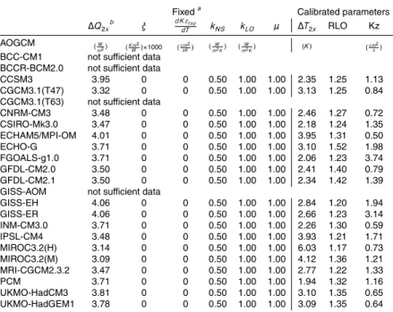
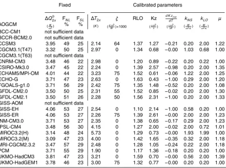
3.1.1 Calibrated parameters

In the first calibration exercise (“calibration I”), only three key parameters were opti-mized, namely the climate sensitivity ∆T2x, the equilibrium land-ocean warming ratio

RLO and the vertical thermal diffusivity Kz in the ocean. Kz has a large influence on

5

the ocean heat uptake efficiency. In the second and third calibration exercises, five additional parameters in MAGICC were optimized to match the AOGCM temperature and heat-uptake results. As in any calibration exercise with multiple parameters, there is the danger of overfitting. Therefore, only a limited set with clearly distinct effects representing different physical mechanisms were chosen out of the large number of 10

MAGICC parameters. Two of the additional five parameters are required to emulate time-varying effective climate sensitivities: namely µ, the ocean to land heat-exchange amplification, which allows the emulation of increasing, but forcing-independent, ef-fective sensitivities (AppendixA4.2); andξ, the forcing-dependency of feedbacks (see

Appendix A4.3). Another parameter, the gradient d K_{d T}ztop, modulates the heat uptake 15

efficiency under higher warming scenarios, by making the vertical diffusivity dependent on the ocean warming (see Appendix A4.7). Furthermore, the two symmetric heat-exchange parameters between land and ocean (kLO) and between the hemispheres

(k_NS) are calibrated, with the latter having no influence on the global-mean warming, but on the hemispheric warming pattern.

20

The parameter space in MAGICC is first sampled randomly with 2000 parameter sets. For each parameter set, up to five parallel runs were done, one for each of the fitted scenarios. Subsequently, the best (in a least-squared sense) parameter set is used to initialize an optimization routine with approximately 1000 iterations to find the parameter combination that minimizes the squared differences between 25

lowpass-filtered AOGCM and MAGICC time series of heat uptake, global, northern land, northern ocean, southern land and southern ocean surface air (2 m)

tempera-ACPD

Full Screen / Esc

Printer-friendly Version Interactive Discussion tures. See AppendixBfor details.

3.1.2 Calibration against idealized CO₂scenarios

In order to successfully emulate the climate response of an AOGCM, its driving forces should be known. This is why idealized experiments, where the forcing is known, are 5

preferred for calibration. For example, MAGICC calibrations for IPCC TAR, as well as feedback paramater calculations by Forster and Taylor (2006), used the first 70 years of the idealized 1% runs. MAGICC 4.2 calibrations for IPCC AR4 used the full-length 1% runs (1pctto2x and 1pctto4x). All 19 CMIP3 AOGCMs considered here provided at least some output for such idealized forcing experiments, assuming an-10

nual 1% increases of CO₂up to doubled and quadrupled concentrations (1pctto2x and 1pctto4x, respectively). Most AOGCMs started these experiment from pre-industrial control runs (picntrl), although four (CCSM3, MRI-CGCM2.3.2, ECHO-G, NCAR PCM) used present-day control runs (pdcntrl). Control-run drift was removed using the re-spective low pass-filtered (1/20 yr−1cutoff frequency) control run segments. Assuming 15

that the CO2 concentration to forcing relationship is logarithmic (IPCC, 1990; Myhre

et al., 1998), the forcing is a ramp-function over 70 (140) years up to its forcing level ∆Q2x at doubled (or quadrupled) CO2 concentrations. ∆Q2x is estimated to be

3.71 Wm−2 (Myhre et al., 1998), although AOGCMs show a relatively large variation (see Table 10.2 in Meehl et al.,2007). Where available, model-specific ∆Q2x values

20

were used during the calibration exercise (see TablesB1andB2). 3.1.3 The difficulty posed by unknown radiative forcing

The inherent difficulty with calibrating MAGICC paramaters to the multi-forcing output data, and the reason why this approach has not been used previously, is the large uncertainties in the actual forcings. Modeling groups took into account different sets 25

ACPD

Full Screen / Esc

Printer-friendly Version Interactive Discussion for the forcings in common, the quantitative information of the actual effective forcings

within AOGCMs is rather limited, mostly restricted to CO₂forcings at doubled CO₂ con-centrations. The first study addressing this shortcoming in a comprehensive manner is the one by Forster and Taylor (2006), who diagnosed the effective forcings. Nei-ther forcings nor efficacies can be diagnosed from the currently available AOGCM data 5

without making additional assumptions, though; for example, with regard to the models’ effective climate sensitivities (Forster and Taylor,2006).

In the present study, given these limitations, we use informed guesses for the individual model forcings. Only the matching set of radiative forcing agents (see Table 2) was applied for each AOGCM using default efficacies (see http://www.

10

atmos-chem-phys-discuss.net/8/6153/2008/acpd-8-6153-2008-supplement.pdf). These reconstructed forcing time-series are hence not identical to the diagnosed forcings given byForster and Taylor(2006). In case of the GISS models, the modeling group provided an independent estimate of the radiative forcing (Hansen, 2005, personal communication as reported in Forster and Taylor,2006), which agrees well 15

with the net effective forcing series used for calibration here (see Fig.2b).

A further step in this study provides insights into how the AOGCM responses might have changed if all AOGCMs had used all forcing agents in their integrations. Unifying the starting years of the emulations to 1750, completing the set of forcings, adjusting historical volcanic forcing to a historical zero mean, and coupling an interactive carbon 20

cycle are several steps taken here in the attempt to produce projections. The full-forcing time series applied here in MAGICC differ from the full-forcing time-series applied in MAGICC 4.2 for IPCC AR4 in particular towards the end of the 21st century (see Fig.2), primarily because of our revised assumption on individual aerosol contributions to the indirect aerosol effects followingHansen et al.(2005) (see AppendixA3.6for details). 25

Figure2highlights the different forcing series for two of the 19 emulated CMIP3 mod-els. The forcings used in IPCC AR4 for the projections with MAGICC 4.2 (calibrated only to idealized scenarios) are in these two cases higher than the diagnosed forcings by (Forster and Taylor,2006) (hereafter referred to as “F&T”). Across all AOGCMs, the

ACPD

Full Screen / Esc

Printer-friendly Version Interactive Discussion mean MAGICC 4.2 forcing series are, however, in close agreement to the respective

multi-model means of the diagnosed F&T forcings, as shown in Fig.9. The “like-with-like” forcings used for calibrations in this study tend to be lower as are the full forcing series used for projections. A more detailed discussion of the MAGICC 4.2 forcing as-sumptions and emulations can be found in Sect.5.1and Fig.9. Forcing assumptions 5

for MAGICC 6.0 made in this study are presented below. The forcing resulting from these assumptions are compared to the diagnosed F&T forcings in Fig.7together with the respective MAGICC 6.0 temperature responses (see Sect.4.4).

3.1.4 Special cases for multi-forcing calibration

Within the forcing agent sets, MAGICC applies forcing histories whose mag-10

nitude from 1750 to 2005 is consistent with the central estimate pro-vided by IPCC AR4 (see http://www.atmos-chem-phys-discuss.net/8/6153/2008/

acpd-8-6153-2008-supplement.pdf or Table 2.12 inForster et al.,2007). The four ex-ceptions are:

Firstly, for volcanic forcing, the amplitude was adjusted for each AOGCM that in-15

cluded volcanic forcing, so that the amplitude in net effective (shortwave and longwave) volcanic forcing is approximately matched as detected byForster and Taylor(2006). A too strong negative amplitude would result in a too high sensitivity ∆T2x, and hence

too warm future MAGICC response, because the chosen goodness of fit statistic, the squared differences, give substantial weight to the larger deviations during strong vol-20

canic forcing events. To minimize the effect of mismatching volcanic forcing series a low pass filter was applied within the optimization routine. The scaling factor for vol-canic forcing was determined to be lower than unity for all models (ranging from 0.2 for INM-CM3.0 and MRI-CGCM2.3.2 to 0.7 for most models). See Table2.

Secondly, CO2related forcing is modeled slightly differently compared to other

forc-25

ing agents: as for the idealized scenarios, the parameter that scales CO2forcing ∆Q2x

is set to its AOGCM-specific value during the calibration exercise (see Eq. A36 and

ACPD

Full Screen / Esc

Printer-friendly Version Interactive Discussion concentrations according to the Bern reference cases provided in the IPCC TAR, these

CO2 concentration scenarios are prescribed in MAGICC when trying to match the

AOGCM output for the SRES scenarios B1 and A1B. Prescribing CO2concentrations

instead of emissions has the additional benefit of keeping the calibration of the car-bon cycle (see following Sect.3.3) strictly separate from the calibration of the climate 5

response.

Thirdly, a special case is the second indirect aerosol effect, characterized by de-fault in IPCC AR4 (Forster et al.,2007) as an efficacy enhancement to the first indirect aerosol effect. For AOGCMs that only included the first indirect effect (ECHAM5/MPI-OM, ECHO-G, IPSL-CM4, UKMO-HadCM3), the second effect is ignored during the 10

calibration exercise. For the GISS-EH and GISS-ER models, which only included the second indirect effect (see Table 10.1 inMeehl et al.,2007), a forcing was assumed of the same magnitude as IPCC AR4’s best estimate of the first indirect aerosol ef-fect (−0.7 Wm−2with efficacy 0.9). For the three models MIROC3.2 (hires), MIROC3.2 (medres) and HadGEM1 that are reported to have included both indirect aerosol ef-15

fects, the efficacy of the first indirect effect has been assumed as 1.5 (default 0.9; i.e., the second indirect effect is assumed to enhance the first indirect effect by 67%) during the calibration exercise following the (very uncertain) efficacy estimates dis-cussed in IPCC AR4 (see Sect. 2.8.5.5 in Meehl et al., 2007 as well as http://www.

atmos-chem-phys-discuss.net/8/6153/2008/acpd-8-6153-2008-supplement.pdf). 20

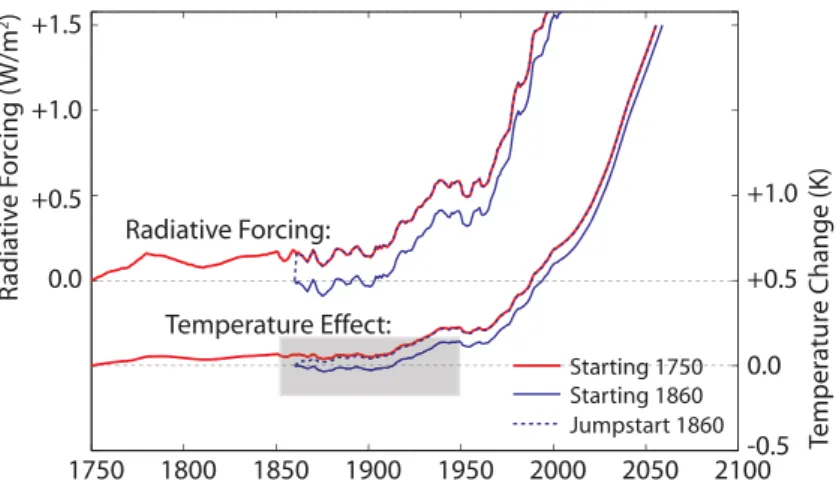
Fourthly, the last issue relates to the “cold start problem” (Hasselmann et al.,1993). Rather than starting in 1750, the reference year for radiative forcings, modeling groups chose years in between 1850 and 1900 as a starting point for the 20th century inte-grations (20c3m runs). Unfortunately, it is not documented how (or if) the AOGCM modeling groups handled any forcing differences between 1750 and the respective 25

starting year. For example, in the default forcing series applied here (excluding vol-canic forcing), a slight forcing increase of roughly +0.2 Wm−2 occurred between 1750 and 1860. Modeling groups could have applied a “jump start”, so that the model is subject to a step forcing increase in the starting year (see Fig.3). Alternatively, models

ACPD

Full Screen / Esc

Printer-friendly Version Interactive Discussion could be driven by radiative forcing changes since their starting year only, neglecting

any forcing changes between 1750 and their starting year. Judging from their temper-ature evolutions, it is assumed here that AOGCMs were initialized with zero forcing in their 20c3m starting year, not in regard to 1750, given that no significant temperature increases are apparent in the early 20c3m runs (cf. case “Starting 1860” in Fig.3). 5

The effect of these different initializations is small in light of the overall projection un-certainties, though still important in order to derive optimal calibrations for individual model response characteristics. For both the climate and carbon cycle models, the only exception is the Hadley C4MIP carbon cycle model, whose temperature evolution suggests that it has been subject to a “jump start” in forcing. Such “jump start” ini-10

tializations have been used earlier as well–as documented inJohns et al.(1997) (see Fig. 30a therein).

3.2 Harmonizing the forcings

There are substantial uncertainties in the forcing magnitudes and their evolution over time. Here, we ensured that the forcing evolutions for each gas, aerosol 15

or albedo effect, are consistent with the point forcing estimates in year 2005 pro-vided in the IPCC AR4 see http://www.atmos-chem-phys-discuss.net/8/6153/2008/

acpd-8-6153-2008-supplement.pdf and Table 2.12 in Forster et al. (2007). We also began each emulation case using MAGICC in 1750 (see Fig.3). An additional change was to adjust the forcing for CO2. As discussed byCollins et al.(2006), radiative

forc-20

ing parameterizations in GCMs can result in substantial deviations from the line-by-line radiative transfer schemes. These deviations are, for example, apparent in the ∆Q2x

values, with values ranging from 3.09 to 4.06 Wm−2 across the AR4 AOGCMs (see first column of Table B3). To remove these differences we used a central estimate of 3.71 Wm−2 (Myhre et al.,1998) consistent with line-by-line models (Collins et al., 25

2006), although it is recognized that there is some uncertainty in the “true” CO2

forc-ing. Finally, instead of using the prescribed CO2 concentrations, we generated these

ACPD

Full Screen / Esc

Printer-friendly Version Interactive Discussion following Sect.3.3) – thereby replacing the prescribed CO₂concentrations.

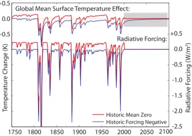
The following paragraph highlights one of the many forcing adjustments, namely the volcanic forcing. Judging from their temperature evolutions, CMIP3 AOGCMs that in-cluded a non-zero volcanic forcing (see Table2), applied volcanic forcing as negative forcing only, which leads to an initial cooling of the global-mean temperatures after 5

the runs branched off from the pre-industrial control simulations. This is an initializa-tion problem, which leads to an artificial cooling of the 20th century simulainitializa-tions (see Fig.4). Furthermore, rather than prescribing a future cooling according to the historical mean, future volcanic forcing is typically assumed zero in the AOGCMs. This leads to a rebound effect with a slight additional warming for 21st century temperatures relative 10

to the base period 1980–1999. Thus, the AOGCMs which did include volcanic forcing are representing a temperature projection for a volcanic-free future, in which a rebound effect is appropriate, although the cooling after initialization is still problematic. Note that the HadCM3 model data stored at PCMDI seems not to have included volcanic forcings in their IPCC AR4 runs (in contrast to the information provided in Table 10.1 15

of Meehl et al., 2007). The approach taken here in the emulations after the forcing adjustments, is attempting to provide best-guess future warming projections including natural forcing, i.e., a mean volcanic cooling and a mean solar forcing according to the recent 100-year and 11-year history, respectively. The benefit of adjusting the historical volcanic forcing series to a mean zero is that the initialization problem is addressed. 20

Keeping a future volcanic mean zero has in turn the benefit that the dependence of future projections on past volcanic forcing assumptions is minimized, i.e., there is no rebound effect. Some AOGCMs, e.g. some HadCM3 runs (J. Lowe, personal commu-nication, 2007; see as well Fig. 1 in Stott et al.,2000), do in fact apply volcanic forcing with a historical zero mean and zero future (see Fig.4).

25

3.3 Calibrating the carbon cycle

The following section details the procedures for calibrating the MAGICC carbon cycle to ten of the eleven carbon cycle models that took part in the C4MIP intercomparison

ACPD

Full Screen / Esc

Printer-friendly Version Interactive Discussion project (Friedlingstein et al.,2006).

MAGICC’s carbon cycle model (see Fig.13) was calibrated in two consecutive steps. In a first step, the climate sensitivity (∆T2x) was derived by prescribing the C4MIP

mod-els’ CO2 concentrations (for runs that included temperature feedbacks on the carbon

cycle) and calibrating MAGICC’s climate sensitivity for default climate module settings 5

to obtain optimal (least squares) agreement with the C4MIP temperature projection (see TableB4). Subsequently, MAGICC’s main carbon cycle parameters were adjusted in order to optimally match the C4MIP model-specific carbon fluxes and pool sizes for both the feedback and non-feedback cases (total of 14 time-series).

The initial MAGICC carbon fluxes were obtained from the available C4MIP datasets, 10

specifically the net primary productivity (NP Pini) and total heterotrophic respiration

(P Rini comprising R, Qa and U). A constant partitioning (45:55) is assumed for the

initial carbon pool sizes of the detritus (Dini), and soil box (Sini), as only the

aggre-gated dead carbon pool is provided for the C4MIP models. C4MIPs initial living carbon pool is equated to MAGICC’s plant (Pini) carbon pool. The start year for fertilization

15

and temperature effects has been assumed to be the first year of the available C4MIP dataseries (first model years ranging from 1765 to 1901; see TableB4.)

Using these initial conditions for carbon fluxes and pools, thirteen MAGICC carbon cycle parameters were calibrated. The semi-automatic procedure involves 2000 ran-domly drawn parameter sets, each run once for the coupled (i.e., including temperature 20

feedbacks) and once for the uncoupled (excluding temperature feedbacks) scenarios. The “best match” parameter set was then chosen as initialization to an automated optimization procedure that fulfils a pre-selected error tolerance criterion after approx-imately another 1000 iterations. By adjusting the thirteen MAGICC parameters, the procedure minimizes the weighted least-squares differences between MAGICC and 25

14 available time series; namely, the air-to-land, air-to-ocean, Net Primary Produc-tion (NPP), and heterotrophic respiraProduc-tion (R, QaandU) fluxes, as well as the living and

dead carbon pools and CO2concentrations for both the with-feedback and no-feedback

ACPD

Full Screen / Esc

Printer-friendly Version Interactive Discussion The three ocean carbon cycle parameters involved in the calibration are: a) the CO₂

gas exchange rate k (yr−1) between the atmosphere and the upper mixed ocean layer (Eq. A22); b) the temperature sensitivity α_T of the sea surface partial pressure (see Eq.A28); c) a scaling factorγ to scale the impulse response function r_t′for the inorganic carbon perturbation in the mixed layer (so that rt=γrt′/(γr

′

t+(1−r

′

t)) for times lower

5

than one year and a constant scaling factorγ′=(r_t=1/r_t=1′ ) for longer response times, i.e., r_t=γ′r_t′ for t>1. The transition year for the scaling factor is chosen to match the

transition time between the initial polynomial and subsequent exponential expression in the impulse response function representing the 3-D-GFDL model. This particular two-part scaling of the impulse response function has been chosen to allow a linear scaling 10

over medium and long timescales (cf. Fig. 7b inJoos et al.,1996), while ensuring a continuous impulse response function from year zero onwards.

The calibrated terrestrial carbon cycle model parameters determine the flux parti-tion inside MAGICC; namely, the fracparti-tion of the plant box flux L going to the detritus

box(φH), the fraction of the detritus box outbound fluxQ going to the soil box (qS). The

15

no-feedback runs were used as well to estimate the fertilization parametersβ_mandβ_s, whereβm refers to whether a standard lognormal formulation for fertilization is used

(βm=1.0), or the rectangular hyperbolic formulation (βm=2.0), or any linear

combina-tion of these two formulacombina-tions (1.0<β_m<2.0). β_s denotes the fertilization factor itself (see Sect.A1.1and Eq.A20). The temperature feedback parametersσi of the carbon

20

fluxes NPP,Q and U (cf. Fig.13) were estimated by matching the difference between the with-feedback and no-feedback runs.

4 AOGCM calibration results

This section gives the results of the three calibration exercises employed here to repli-cate the climate response characteristics of the AOGCMs (Sects.4.1, 4.2, and 4.3). 25

The forcing and temperature effects of the AOGCM-specific forcing adjustments are given in Sect.4.4. Section4.5provides the results of the carbon cycle calibrations.

ACPD

Full Screen / Esc

Printer-friendly Version Interactive Discussion 4.1 Calibration Method I – as in the AR4

Here we fit the idealized CO2-only scenarios 1pctto2x and 1pctto4x, using only the

three most important MAGICC parameters; the equilibrium climate sensitivity (∆T2x),

the equilibrium land-ocean warming ratio (RLO), and the vertical diffusivity in the ocean (Kz) (see TableB1).

5

This simple calibration approach enables the emulation of the evolution of global-mean temperatures for the idealized scenarios relatively well for most AOGCMs. The root mean square errors (RMSE) between emulations and the AOGCMs are well be-low 0.2◦C for the 1pctto2x and 1pctto4x scenarios for all but four models (UKMO HadGEM1, CCCma CGCM3.1(T47), GFDL CM2.0 and MPI ECHAM5), as shown in 10

Fig. 5a. As can be expected, the SRES and “commit” multi-forcing scenarios are less well emulated for almost all models, as their information was not used to derive the op-timal parameter settings for ∆T2x, RLO and Kz. This discrepancy between emulations

and AOGCM multi-forcing runs is substantial for three out of the 19 emulations show-ing RMSE values higher than 0.35◦C. On average across all models and scenarios, the 15

RMSE is 0.21◦C (see Fig. 5a).

In order to put this RMSE value of 0.21◦C in perspective, it is here compared to the equivalent goodness of fit statistic, if a single AOGCM’s projections were simply approximated by the global-mean temperature time-series of another randomly drawn AOGCM for the same scenario. This comparison is motivated by the common practice 20

in many studies to make inferences from single AOGCMs, often implying that a single AOGCM is representative for a wider range of other AOGCMs. Thus, for this compar-ative measure of inter-model uncertainty, we computed the average RMSE between global-mean temperature series for all permutations of CMIP3 AOGCMs applying the same lowpass filter as used for the calibrations (1/20 yr−1cutoff frequency), taking into 25

account the full overlapping time-periods between any pair of AOGCMs. The resulting RMSE is 0.46◦C across the multi-forcing and idealized scenarios, more than twice as high compared to the RMSE of emulations following the “calibration I” procedure.

ACPD

Full Screen / Esc

Printer-friendly Version Interactive Discussion It is noticeable that some AOGCMs show features in their idealized scenario runs

(1pctto2x and 1pctto4x), that cannot possibly be emulated satisfactorily by only opti-mizing the three parameters ∆T2x, RLO and Kz. For example, a larger best-fit effective

climate sensitivity for the higher forcing 1pctto4x run than for the 1pctto2x run is appar-ent in the MPI ECHAM5 simulation, after these runs diverge in year 70 of the model 5

integration (see Fig.1, and discussion in Sect.5.2). A constant climate sensitivity ∆T2x

is thus not able to match both scenarios satisfactorily. The best-fit constant climate sensitivity will be in-between the effective sensitivities for the 1pctto2x and 1pctto4x runs. Indeed, the “calibration I” procedure gives a climate sensitivity of 3.95◦C (see TableB1), which is in between the effective sensitivities of 3.5 and 4.2◦C towards the 10

end of the 1pctto2x and 1pctto4x scenarios, respectively (see Fig.1). 4.2 Calibration Method II – using additional parameters

For some AOGCMs, the use of additional parameters in the fitting exercise did not improve the goodness of fit (MIROC3.2(hires), GISS-EH and FGOALS-g1.0). For other, the fit was improved markedly. For example, the RMSE is halved for NCAR CCSM3 and 15

GISS-ER (see 1pctto2x and 1pctto4x scenarios in Fig. 5a and c). The enhanced ability to match the idealized scenarios of the MPI ECHAM5 model is most noticeable: under “Method I”, the RMSE values were 0.30◦C and 0.43◦C. The idealized scenarios are now emulated with an RMSE of 0.15◦C and 0.11◦C– primarily due to the ability of MAGICC under “Method II” to simulate time-varying effective sensitivities for the 1pctto2x and 20

1pctto4x scenarios (see Fig.1). The idealized scenarios as well as the multi-forcing scenarios are more accurately emulated, so that the goodness of fit ranking for MPI ECHAM5 improved (see Fig. 5).

In summary, the match to the idealized scenarios improved for all those models that provided 1pctto2x and 1pctto4x data. The models where there was no improvement, 25

see above, were those that provided only 1pctto2x data. The emulation skill for the multi-forcing scenarios, which were – as in “calibration I” – not used for “calibration II”, was only slightly enhanced in most cases. The average RMSE across all scenarios

ACPD

Full Screen / Esc

Printer-friendly Version Interactive Discussion and models is 0.188◦C (see Fig. 5a and c), slightly improved from the 0.206◦C that

resulted from the “calibration I” procedure.

4.3 Calibration Method III – from CO₂-only to multi-forcing

While the inclusion of additional parameters under the “calibration II” procedure markedly improved the fit to the idealized experiments, the performance of the em-5

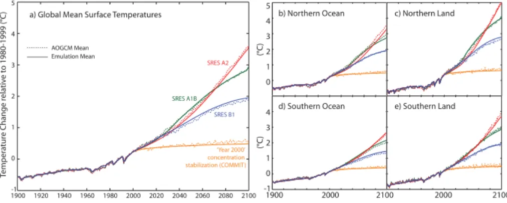
ulations for the multi-forcing runs is still imperfect. Obviously, the emulation quality for SRES scenarios enhances, if a goodness of fit statistic for these SRES scenarios is included in the optimization routine. Analyzing the global-mean as well as the hemi-spheric land and ocean average temperatures relative to the control run simulations reveals a remarkable consistency between the mean of the emulations and the mean 10

of the AOGCM runs under the “calibration III” strategy (see Fig.6and Table3).

For individual AOGCMs, the deviations over the full scenario duration are small, mostly <0.2◦C (see Fig. 5f). The largest deviation in global means of up to 0.5◦C is for the model, for which the calibrated MAGICC was least capable of simulating their temperature under the multi-forcing scenarios, namely CNRM CM3. The emulations of 15

CNRM CM3 show most clearly what is apparent as well for eight other AOGCMs (GISS-ER, MIROC3.2 (medres), NCAR PCM1, MPI ECHAM5, MRI CGCM2.3.2A, IPSL-CM4, INM-CM3.0 and HadGEM1), namely that the idealized scenarios are emulated too warm and the multi-forcing runs too cold or vice versa (see Fig. 5f). In the case of CNRM CM3, this likely points to an underestimation of the net forcing in the multi-20

forcing runs or overestimation of the CO2forcing in the idealized scenarios. The

aver-age RMSE across all scenarios and models further decreased to 0.172 K, so that the intermodel uncertainty RMSE of 0.46◦C is more than 2.5 times higher compared to the uncertainty introduced by the emulations of an individual AOGCM. The mean across all AOGCM emulations compared to the mean of the original AOGCM’s global tem-25

perature evolutions has an RMSE of 0.053◦C (averaged across all multi-forcing runs 2000–2100). This highlights that the emulations of the multi-model ensemble mean is substantially more robust than emulating a single AOGCM and associated with very

ACPD

Full Screen / Esc

Printer-friendly Version Interactive Discussion minor biases, if any (see Fig.6).

As the SRES A2 scenario has not been used for calibration, but left as an indepen-dent test case for the validity of the emulations, the emulation skill in comparison to the other multi-forcing runs is of interest. The performance of the emulations for the high SRES A2 scenario is similar to the other two SRES scenarios B1 and A1B that 5

were taken into account for the calibration (average RMSE A2: 0.175◦C; A1B: 0.190◦C, B1: 0.168◦C; see Fig. 5e). This is encouraging as it supports the assumption that emulations for other emissions scenarios approximately reflect what AOGCMs would project.

Again, it is valuable putting these errors introduced by the emulations in perspective. 10

The inter-model uncertainties between AOGCMs in regard to global-mean tempera-tures towards the end of the 21st century (2090–2099) to SRES scenarios are roughly 40%, when expressed as double standard deviation divided by the multi-model en-semble mean (B1:49%, A1B:41%, A2:26%) (cf. Knutti et al., 2008). In comparison, the mean relative errors introduced by the emulations are substantially smaller, i.e., 15

less than 2.2% for the ensemble means (B1:2.2%, A1B:−1.0%, A2:−0.8%) and, on average, 7% for individual AOGCM emulations over 2090–2099 relative to 1980–1999 (B1:9%, A1B:6%, A2:6%). Comparing these 2090–2099 warmings between emula-tions and AOGCMs relative to AOGCM starting years reduces differences further, as well because the uncertainties introduced by the strong Pinatubo volcanic forcing in 20

the 1980–1999 base period are circumvented: Individual AOGCMs in the last decade of the 21st century are now matched in average with a mean relative error of only 6% (B1:5%, A1B:5%, A2:7%). The better half of emulation and AOGCM pairs show deviations of only 3% on average (B1:3%, A1B:2%, A2:5%).

4.4 Harmonized forcing results 25

In this section we consider the effects on temperature that arise because different AOGCMs used different forcings (both historically and in the future), as well as dif-ferent starting dates. Even if all AOGCMs had the same physics (i.e., the same climate

ACPD

Full Screen / Esc

Printer-friendly Version Interactive Discussion sensitivity, ocean mixing, etc.), these differences would cause the projected climate

changes to diverge. We analyze this effect by applying a common set of forcings to the different MAGICC emulations, model by model, and compare the resulting projections with those that arise when only model-specific forcings are used (see Fig. 2). As a representative example, we consider results for the A1B scenario.

5

The starting point of the analysis is the set of AOGCM specific “like-with-like” forc-ings applied for calibrating MAGICC parameters (see Table2). Comparing the mean of these efficacy-adjusted forcing series used for calibration with the mean of the di-agnosed F&T forcings reveals a close match up to the middle of the 21st century (see first sub-panel indicated with black circled “1” in Fig.7a). Thereafter, the “like-with-like” 10

forcings assumed here turn lower than the diagnosed F&T forcings. This difference might at least partially be due to an overestimation of the effective F&T forcings to-wards the second half of the 21st century. The reason for the potential overestimation of diagnosed forcings could be thatForster and Taylor (2006) assumed constant cli-mate sensitivities, esticli-mated from the first 70 years of the idealized forcing scenarios. 15

If in fact effective climate sensitivities are increasing in some models over time, this method would lead to an underestimation of the effective climate sensitivity at the end of the 21st century and hence an overestimation of the forcings. There are two factors supporting this hypothesis. Firstly, in the idealized scenarios, for which the forcing is better known, the diagnosis of effective climate sensitivities (see equation3) reveals 20

increasing climate sensitivities for higher forcing levels for a number of models - as shown in Fig.1for CCSM3 and ECHAM5/MPI-OM. Secondly, continuing the analysis byForster and Taylor(2006) beyond 2100 suggests increasing diagnosed forcings for some models, inconsistent with the fact that forcings should be constant after 2100 by definition of the scenarios (Meehl et al.,2005a).

25

The close match between the A1B forcings assumed here and the diagnosed F&T forcings up to the middle of the 21st century is reflected in a close match of the global-mean temperatures. Also, the emulated global-mean temperature perturbations in MAGICC 6.0 using the “like-with-like” forcings are within 0.1◦C of the AOGCM mean throughout

ACPD

Full Screen / Esc

Printer-friendly Version Interactive Discussion the whole emulation period, which tends to support our forcing assumptions compared

to the diagnosed F&T forcings (see black circled “1” in Fig.7b). Relative to the base period 1980–1999, the difference in projected warming for 2090–2099 between the MAGICC emulations and the AOGCMs is 0.02◦C or less than 1% (cf. column AOGCM and IIIa for “Period 2” in Table3).

5

One of the difficulties interpreting the AOGCM results for the past is that modelling groups assumed different starting years, in which the 20th century simulations (20c3m) diverge from the pre-industrial control runs. Unifying these starting years to 1750 shifts the forcing to higher values. This is because the forcing increments of CO2 and other

considered forcing agents between 1750 and the starting years, e.g. 1850 or 1900, are 10

now taken into account (see Fig.3and “2” in Fig.7a). Had all AOGCMs started their simulations in 1750, their temperature projections for the 21st century could be ex-pected to be approximately 0.1◦C warmer relative to 1750 (see “2” in Fig.7b), although this effect almost vanishes when taking differences to the 1980–1999 base period (see “2” in Fig.7c).

15

In the next step, all AOGCM emulations were now run with complete and unified forcings. Specifically, if an AOGCM had left out a specific forcing agent (e.g. indi-rect aerosol effects or tropospheric ozone), the climate module has been calibrated by taking account of this omission. Completing and unifying the missing sets of radia-tive forcing agents in each AOGCM simulation (see Table2), unifying the CO₂ forcing 20

(∆Q2x=3.71 Wm−2) and adjusting the historical volcanic forcing to a zero mean has a

significant effect on the applied forcing (see “3” in Fig.7a).

These numerous forcing adjustments have obviously a pronounced effect on the emulated temperatures. Relative to the starting years of the emulations, the tempera-tures drop by around 0.4◦C for much of the 21st century (see “3” in Fig.7b). However, 25

when taking differences to the base period 1980–1999, the 21st century temperatures only cool by 0.1◦C in average (see “3” in Fig. 7c). Hence, the partial omission of aerosol effects and volcanic forcings did not result in a significant projection error for 21st AOGCM temperature projections under the SRES A1B scenario in IPCC AR4,