HAL Id: hal-00305133
https://hal.archives-ouvertes.fr/hal-00305133
Submitted on 21 Feb 2008
HAL is a multi-disciplinary open access
archive for the deposit and dissemination of
sci-entific research documents, whether they are
pub-lished or not. The documents may come from
teaching and research institutions in France or
abroad, or from public or private research centers.
L’archive ouverte pluridisciplinaire HAL, est
destinée au dépôt et à la diffusion de documents
scientifiques de niveau recherche, publiés ou non,
émanant des établissements d’enseignement et de
recherche français ou étrangers, des laboratoires
publics ou privés.
Prediction of littoral drift with artificial neural networks
A. K. Singh, M. C. Deo, V. Sanil Kumar
To cite this version:
A. K. Singh, M. C. Deo, V. Sanil Kumar. Prediction of littoral drift with artificial neural networks.
Hydrology and Earth System Sciences Discussions, European Geosciences Union, 2008, 12 (1),
pp.267-275. �hal-00305133�
© Author(s) 2008. This work is distributed under the Creative Commons Attribution 3.0 License.
Earth System
Sciences
Prediction of littoral drift with artificial neural networks
A. K. Singh1, M. C. Deo1, and V. Sanil Kumar2
1Department of Civil Engineering, Indian Institute of Technology, Bombay, Mumbai 400 076, India 2Ocean Engineering, National Institute of Oceanography, Dona Paula, Goa 403 004, India
Received: 11 June 2007 – Published in Hydrol. Earth Syst. Sci. Discuss.: 31 July 2007 Revised: 10 December 2007 – Accepted: 18 January 2008 – Published: 21 February 2008
Abstract. The amount of sand moving parallel to a coastline
forms a prerequisite for many harbor design projects. Such information is currently obtained through various empirical formulae. Despite so many works in the past an accurate and reliable estimation of the rate of sand drift has still remained as a problem. The current study addresses this issue through the use of artificial neural networks (ANN). Feed forward networks were developed to predict the sand drift from a va-riety of causative variables. The best network was selected after trying out many alternatives. In order to improve the accuracy further its outcome was used to develop another network. Such simple two-stage training yielded most sat-isfactory results. An equation combining the network and a non-linear regression is presented for quick field usage. An attempt was made to see how both ANN and statistical re-gression differ in processing the input information. The net-work was validated by confirming its consistency with un-derlying physical process.
1 Introduction
Littoral drift indicates movement of sediments parallel to a coastline caused by the breaking action of waves. Ocean waves attacking the shoreline at an angle produce a current parallel to the coast. Such longshore current is responsible for the longshore movement of the sediment (Komar, 1976). Littoral drift poses severe problems in coastal and harbor op-erations since it results in siltation of deeper navigation chan-nels due to which ships cannot enter or leave the harbor area. An accurate estimation of the drift is needed in order to know the amount of excavation required so that corresponding bud-getary provisions could be made in advance. Unfortunately
Correspondence to: M. C. Deo
(mcdeo@civil.iitb.ac.in)
this is easier said than done because the underlying physi-cal process is too complex to model in the form of mathe-matical equations – either parametric or differential. Despite this, workable empirical formulae that relate the drift to a set of causative variables are currently in use. They are based on collection of measurements made in the field or on a hy-draulic model followed by a curve fitting exercise. The tech-nique of fitting normally employed is non-linear statistical regression. It is well known by now that the soft tools like artificial neural networks (ANN) many times provide bet-ter albet-ternative to the statistical methods (see e.g. ASCE Task Committee, 2000; Kambekar and Deo, 2003) and hence a variety of investigators have applied the technique of ANN to solve problems in coastal engineering. These works typ-ically include (a) wave height predictions (Deo and Naidu, 1999; Tsai et al., 2002; Makarynskyy, 2004; Altunkaynak and Ozger, 2004; Tolman et al., 2004), (b) evaluating tidal levels and timings of high and low water (Deo and Chaud-hari, 1998; Lee, 2004), (c) predicting sea levels (Vaziri, 1997; Cox et al., 2002), (d) forecasting wind speeds (Lee and Jeng, 2002; More and Deo, 2003) (e) establishing estuarine characteristics (Grubert, 1995) and (f) predicting coastal cur-rents (Babovic et al., 2001), (g) other met-ocean parameters (Krasnopolsky et al., 2002; Refaat, 2001). A comprehensive review of ANN applications in related areas can be seen in Jain and Deo (2006). The application of ANN however gen-erally suffers from problems like lack of guarantee of suc-cess, arbitrary accuracy, and difficult choices related to train-ing schemes, architectures, learntrain-ing algorithms, and control parameters. Any new application of the ANN that addresses these issues therefore deserves attention of the potential user community. The current study is directed along this line and discusses an application of the ANN to determine the littoral drift. Novel methods of network training are employed. An equation combining the ANN and the non-linear regression is presented for those desirous of making hand calculations. An attempt is made to see how both ANN and the statistical
268 A. K. Singh et al.: Prediction of littoral drift
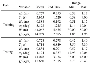
Table 1. Statistics of the training and testing data set.
Data Range
Variable Mean Std. Dev. Min. Max.
Training Hs(m) 0.767 0.255 0.33 1.17 Tz(s) 5.975 1.520 0.58 9.00 Hb(m) 0.888 0.192 0.51 1.17 αb(deg) 5.198 1.725 1.14 10.04 W (m) 41.067 4.635 30.00 50.00 Q (kg/s) 14.969 7.585 1.86 31.96 Testing Hs(m) 0.728 0.278 0.42 1.40 Tz(s) 4.714 0.849 3.50 7.30 Hb(m) 0.834 0.201 0.52 1.17 αb(deg) 4.124 6.377 −17.93 10.06 W (m) 41.048 3.074 35.00 45.00 Q (kg/s) 15.650 7.015 5.78 26.43
regression differ in processing the input information. The consistency of the network with underlying physical process is further checked.
2 Network development
2.1 Training schemes
Most of the previous applications of ANN to water flows in-volved use of the feed forward network (ASCE Task Com-mittee, 2000). The current study was also based on the same. Both multi-layered perceptron network (MLP) as well as its variant radial basis function (RBF) was used. Training of the MLP was achieved with the help of alternative learn-ing schemes like Conjugate Gradient Polak-Rebiere Update (CGP), Powell Beale Restarts (CGB), Scaled Conjugate Gra-dient (SCG), One Step Secant algorithm (OSS) and Resilient Backpropagation (RP). Demuth et al. (1998) may be referred to understand details of these training algorithms.
2.2 The database used
The network was trained with the help of field observations. The location belonged to a four-km stretch of the coast off Karwar along the western coast of India. These field mea-surements were done daily from 5 February 1990 to 31 May 1990 by the National Institute of Oceanography at Goa, In-dia. The sediment load was measured along a cross section of the surf zone at six stations at the same time and at a num-ber of points vertically at each station. In each day, the traps were deployed for 6 h during 07:00 to 13:00 h and the average sediment load per hour was calculated. Two different traps were used to measure the littoral drift rates. Mesh traps hav-ing circular openhav-ings were used for measurhav-ing the suspended load transport and streamer traps were used for measuring
0.5 0.6 0.7 0.8 0.9 1 1.1 1.2 1.3 0 5 10 15 20 25 30 35 H b: m Q s : k g /s
Fig. 1. Variation of rate of the drift with breaking wave height. the bed-load transport. The opening of the trap was 0.2 m wide, 0.15 m high, and rectangular in shape. The filter cloth mesh opening size was 90 µm and the opening of the mesh trap was 0.034 m. The procedure of Kraus (1987) was used to determine the total sediment transport and this was based on the trapezoidal rule. The measurements of the significant wave height and average zero cross wave period along with the wave direction corresponding to the spectral peak were made with the help of a WAVEC buoy. The breaking wave height and corresponding angle were derived as per the pro-cedure in Skovgaard et al. (1975) and Weishar and Byrne (1978) and also visually confirmed. The width of the surf zone was measured daily using a graduated rope. The aver-age longshore currents were measured daily (in terms of the distance covered in two minutes) using the Rhodanine-B type dye injected at the trap locations. A standard sieve analysis gave the median size distribution. When all the parameters such as wave height, wave period, wave direction, longshore current speed and direction and sediment load at different trap locations along the surf zone, were not collected in a day due to malfunctioning of instruments or due to overtop-ping of traps, then the data of that day were not used in the analysis. The details on the data collection and the estima-tion of measured sediment load are presented in Kumar et al. (2003). The tides were predominantly semi-diurnal with an average spring tide of 2 m and neap tide of 0.25 m during the measurement period. The longshore current velocities measured at the trap locations varied from 0.1 m/s to 0.6 m/s with an average value of 0.3 m/s. Table 1 shows ranges of the significant wave height (Hs), average zero cross wave period
(Tz), breaking wave height (Hb), breaking angle (αb), surf
zone width (W ) as well as rate of the drift (Q) along with their mean values and standard deviations involved during the training and testing exercises. The rate of littoral drift was found to be randomly varying with the independent causative variables. This is illustrated in the scatter plot of Fig. 1.
Table 2. Effect of changing input on the testing data set.
Input Training algorithm r RMSE (kg/s) MAE (kg/s) Hs, Tz, Hb, αb, W CGB 0.867 3.664 2.929
Hs, Tz, Hb, αb, V RP 0.793 4.443 3.510
Hs, Tz, Hb, αb, d50 RP 0.831 5.137 4.390
2.3 Network formulation
The phenomenon of littoral drift is influenced by a variety of causative factors- some of which could be of importance while some others may not be so influential in determining the rate of drift. The Shore Protection Manual (Department of the Army, 1984) as well as the Coastal Engineering Man-ual (Department of the Army, 2002) list these variables as incident significant wave height (Hs), breaking wave height
(Hb), significant or average zero cross period (Tz), angle of
the wave at the time of breaking (αb), width of the wave
breaking (surf) zone (W ), sediment size (d50), and,
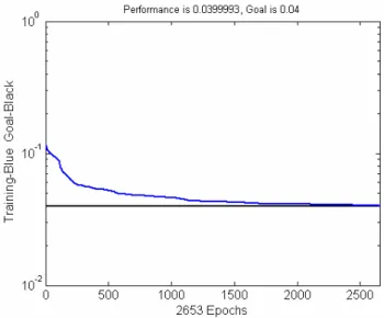
long-shore current (V ). A network with these parameters as in-put and the rate of drift, Q as outin-put was considered. In total 81 input-output patterns were available through the measured data; out of which 75 percent selected randomly were used for training. Such a trained network was tested with the help of remaining 25 percent patterns. A typical plot showing how the training error reduced with increasing number of training epochs is shown in Fig. 2. It is to be noted here that col-lection of all these parameters simultaneously in the fierce oceanic conditions is a difficult task due to variety of instru-ments and equipinstru-ments involved and hence most of the times investigators have to work with a limited sample size. An al-ternative to this is to resort to laboratory measurements. But this is always associated with problems like scale effects and ignorance of complex real sea conditions.
All of the causative variables listed above may not be equally influential in producing the drift at a given location. A sensitivity analysis of the input was done using the prun-ing method in which all causative variables were considered and given as input. The network was trained and the testing performance in terms of the various error measures described subsequently was noted. Thereafter each input was omitted one by one and the training and testing was repeated. This exercise revealed that exclusion of any of the parameters of
Hs, Tz, Hb, and αbresulted in low performance. However it
was also noted that in addition to these if we include W in preference to V and d50 then the best performance is seen.
Table 2 shows resulting performance over the testing pairs (when the best learning algorithm was employed) in terms of the multiple error criteria of the coefficient of correlation (r), root mean square error (RMSE), and mean absolute er-ror (MAE). It is mentioned that random selections of training and testing pairs were done innumerable number of times till
Fig. 2. Error reduction during training (Algorithm: CGB).
the one that produced the best outcome in terms of the error statistics was arrived at.
From Table 2 it is clear that a network that includes the width of the surf zone, W , in addition to that of Hs, Tz, Hb,
and αbgives the best accuracy for testing. However it needs
to be mentioned here that this accuracy resulted after resort-ing to trainresort-ing by alternative schemes like SCG, RP, OSS, CGP, CGB and not by adoption of any one of these randomly. The algorithm of CGB resulted in the best performance. This scheme of training achieves its efficiency using minimum or-thogonality between the current and the preceding error gra-dient. The CGB algorithm performed consistently well for almost all trials.
The number of hidden nodes in case of the above network (input: Hs, Tz, Hb, αb, W ) was 6. This was decided by
tri-als conducted by increasing the number of hidden nodes one by one and every time noticing performance of the trained network by the error statistics and stopping when such per-formance did not change with further addition of the hidden nodes. A scatter plot checked the testing performance of this network (Fig. 3), which further qualitatively indicates a sat-isfactory result.
270 A. K. Singh et al.: Prediction of littoral drift
Fig. 3. Predicted v/s observed drift (traditional ANN).
Fig. 4. Comparison of empirical formulae with observed drift.
3 Regression models
In order to check how the neural network performs vis-`a-vis the statistical regression three new regression equations (linear multiple (LM) as well as non-linear (NL1 and NL2) were fitted to the training set of data. The resulting equations respectively are:
Q = −18.7152 − 13.7319HS−0.3759TZ+39.4895Hb
+0.3455αb+0.2340W (1)
Q = 0.28 × HS(−0.7693)×TZ(−0.0704)×Hb(2.7935)×α(0.0005)b
×W(1.1005) (2)
Table 3. Comparison of the ANN and regression results on the
testing data set.
Scheme r RMSE (kg/s) MAE (kg/s) ANN 0.867 3.664 2.929 LM 0.699 5.356 4.773 NL1 0.799 5.271 3.935 NL2 0.764 5.615 4.019 ln Q = −0.6566 − 1.2978HS−0.0264TZ+3.5802Hb +0.0016αb+0.0283W (3)
The last 3 rows of Table 3 show the testing performance of these regression-fits vis-`a-vis the ANN, which confirms the necessity of employing ANN for this problem in place of the traditional regression (higher r and lower RMSE and MAE). The adequately selected network thus yielded a higher level of accuracy compared with the traditional regression models; the major underlying reasons being, model-free es-timation procedure and flexibility in the mapping process in-volved.
3.1 Traditional formulae
The above study discussed how the network performed vis-`a-vis those statistical regression models that were newly de-rived and based on the especially collected data by authors. Traditionally however most of the harbor and coast develop-ment works in India are carried out by using an empirical equation known as the Coastal engineering Research Centre (CERC) formula and also by the Walton and Bruno equation. The CERC formula (Shore Protection Manual, Department of the Army, 1984) assumes that the drift (Q) is proportional to the longshore energy flux (Pl), i.e.
Q = K.Pl (4)
where K = a dimensionless constant. The flux, Pl, in turn
depends on the sediment characteristics, (like its mass den-sity, ρsand porosity, p), the breaking wave height Hband its
angle αbwith the shore and the wave period T . Specifically
Pl =
1
64π[(ρs−ρw) g (1 − p)]
−1ρ
wg2Hb2T sin 2αb (5)
In the above equation ρwis the mass density of seawater and
g is the acceleration due to gravity.
The Walton and Bruno formula on the other hand relies more on the derived parameters rather than the actual mea-sured ones. The introduction of the surf zone width is also a specialty of this formula. Accordingly the longshore flux (Pls) is given by:
Pls =0.008 (v/v0)[(ρs−ρw) g (1 − p)]−1ρwHbW V (6)
Fig. 5. The two-stage network.
The above equation is based on the assumption that the fric-tion factor is 0.005 and that the theoretical non-dimensional longshore current velocity (v/v0) is calculated with a mixing
parameter of 40%. Equation (6) also uses the actual long-shore current speed V .
The drift predicted by the above formulae was compared with its corresponding value actually measured in the field for the testing data conditions. Figure 4 shows the outcome. It clearly indicates that the field observations of the rate of sediment transport are different than the corresponding val-ues suggested by the two traditional formulae. The empirical constants in these equations were earlier derived on the basis of measurements made at those locations where the coastal environment, geomorphology and topographic characteris-tics were different than the same at the Indian sites. Based on a comparison of the measured values with the commonly used and existing formula, Kumar et al. (2003) had found that the CERC formula and Walton and Bruno formula over predict the longshore sediment transport rate. The difference between the measured and calculated values is attributed due to the use of the empirical formulas developed for the high-energy coast during relatively low wave conditions as the av-erage wave height during the measurement period was 0.8 m. Currently research is on to develop new empirical formulae based on different data sets collected at different parts of the world including the data used in the present study (Bayram et al., 2007).
The unacceptable predictions obtained in the above ex-ercise further confirm the necessity of the ANN or ANN-regression hybrid models (described later) developed in this study.
4 Extended two-stage network
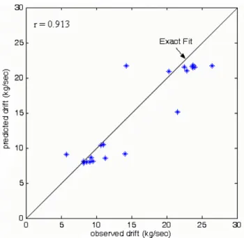
In order to increase accuracy of the network prediction fur-ther the outcome of network (architecture: 5-6-1) was given as input to another network with one input node and one out-put node (and 2 hidden nodes selected after trials as men-tioned earlier in the section: Network Formulation) as shown in Fig. 5. Such a two-stage network, where a cause-effect network carries out the basic function approximation in the beginning and the recycler network later does the fine-tuning, was trained with the help of the training pairs and tested with the help of the testing pairs, as earlier. The testing results (Fig. 6) indicated that such a two-stage network performs much better than the earlier single-stage one, with r as high as 0.913 and RMSE and MAE as low as 3.006 (kg/s) and 2.222 (kg/s) respectively.
The use of two networks made in this way seems to work better than that of an equivalent single network with three or so hidden layers since in the case of the two-stage network a pool of hidden neurons is first allowed to learn indepen-dently and later on by capturing the finer details that may have been left out during the basic learning process of the main network. The first network can be expected to have done major regression, but leaving relatively large difference between the actual output and the evaluated one. The second network may build upon such an outcome (or difference) and may learn the target output more efficiently since now the learning process became more simplified.
272 A. K. Singh et al.: Prediction of littoral drift
Fig. 6. Predicted v/s observed drift (revised ANN) Fig. 6. Predicted v/s observed drift (revised ANN).
5 ANN-regression hybrid model
In the light of the fact that the NL1 regression was next in line in terms of the testing performance (Table 3) and that for quick field applications or for making hand calculations an equation would be preferred by the practitioners rather than the complex matrix of trained weight and bias, a new and simple network with one-input node belonging to the littoral drift rate, Q, given by Eq. (2), or NL1 model, and one output node belonging to the output value of Q was trained and fur-ther tested on the basis of the testing data set. The result was encouraging (r=0.832, RMSE=4.349 (kg/s), MAE=3.411), though not as satisfactory as the two-stage ANN, and this is given in an equation form below:
Q = f (−0.0555f (−16.8QNL1+16.8)
+0.5738f (16.8QNL1−8.4)
+0.312f (16.8QNL1) − 0.9999) (7)
where, QNL1= output from Eq. (2), and in general for any x,
f (x) = [1 + exp(−x)]−1 (8)
The authors also carried out ANN calibration using the n-fold validation in which the total training set was divided into subsets and the training and validation was carried out for varying subset sizes. But this did not provide any further improvement in the testing results. Alternative and probably simpler machine learning methods like the M5 model tree of Quinlan, or instance-based learning methods (for example the k-nearest neighbor) can also be explored, but it is feared that all these methods including the n-fold validation of the ANN may get “saturated” for the given sample size and pro-duce similar results.
Fig. 7a. Input (Hs) processing by ANN.
Fig. 7b. Input (Hs) processing by regression.
6 Consistency in following the physical process
The breaking waves mobilize the sediments that are subse-quently moved by the wave induced longshore current. The parameters which influence the sediment transport rate at a location are breaking wave height, wave period, breaker an-gle, sediment size and the nearshore profile or the surf zone width. The longshore sediment transport in the study area is induced mainly by wave breaking, than due to tide or wind-driven currents, hence the input parameters arrived at after pruning are related to wave breaking. During the study pe-riod, the variations in sediment size were relatively small with median grain size varying from 0.15 to 0.2 mm. Hence inclusion of the sediment size did not yield good results.
The ANN developed by training cannot be put into prac-tice unless its performance after training is found to be con-sistent with the underlying physical process. This may be
Fig. 8a. Input (Hb) processing by ANN.
Fig. 8b. Input (Hb) processing by regression.
viewed as especially necessary when one works with rather limited sample size. A parametric study was therefore per-formed in which one input variable was varied over its full range keeping all other input quantities as constant. The idea was that the variation drawn in this way must match with the one that can be expected from the known physics of the underlying process. Thus increase in magnitude of the wave height should yield larger drift owing to the increase in the re-sulting longshore current. This can be clearly seen in Figs. 7a and 8a which indicate what happens in the trained network when significant wave heights and breaking wave heights be-come higher. Many studies in the past (e.g., Narasimhan and Deo, 1979) have shown that there is only a weak correlation between the wave height Hsand the wave period Tz. A given
Fig. 9. Variation of the drift with wave period in the ANN.
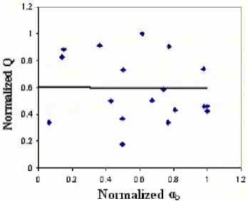
Fig. 10. Variation of the drift with the breaking angle in the ANN.
wave height can occur in association with any value of the wave period and thus can be associated with a range of val-ues of the wave period. However as Hs starts increasing from a low value Tz also increases, but this trend continues only
up to a certain higher value of Hs after which a reverse trend is noticed. Thus very high Hs values usually correspond to some middle range of Tz values. Higher Hs would mean
larger drifts and thus it can be guessed that the maximum drift would correspond to some middle range of Tz values.
Fig-ure 9 confirms this. Similarly higher values of the breaking angle, αb, should mean higher longshore current component
and hence a larger drift. A clear tendency towards this is not seen in Fig. 10 (although a weak trend may be speculated). This may probably be due to a limited range of αbvalues
274 A. K. Singh et al.: Prediction of littoral drift network thus can be seen to be generally consistent with the
physical process of coastal sediment movement.
In order to understand why the ANN performed better than the regression a parametric variation of Q against all causative variables was studied. Figure 7a and b as well as Fig. 8a and b show examples of how the trained network as well as the regression Eq. (2) processed the input of in-creasing Hs and Hb values respectively. The relatively low
spread of points around the fitted line in case of the regres-sion (Figs. 7b and 8b) indicate that the regresregres-sion performs rigid approximations with changing input compared with the ANN, due to which its accuracy drops down.
7 Conclusions
Feed forward networks were developed to predict the rate of littoral drift from a variety of causative variables. The use of a two-stage network system in which a regular network trained in the best possible manner first carries out a cause-effect modeling and another one later on fine tunes its out-come resulted in an improved accuracy of predictions.
New regression Eqs. (1–3) derived in this study can also be used to forecast the value of the littoral drift although with less accuracy than the ANN.
An Eq. (7) combining the ANN and the non-linear regres-sion is presented for quick field usage, although it may not predict the drift with as equal accuracy as that of the ANN.
An analysis showing how both ANN and statistical regres-sion process the input is also presented. It is found that the re-gression performs rigid approximations with changing input compared with the ANN and due to this its accuracy drops. The developed network was found to be consistent with the underlying physical process and generally followed expected trends in the variables of the drift with an increase in the val-ues of causative parameters.
It is recognized that the findings reported in this paper are based on a limited set of field observations and hence it would be desirable to confirm the same further by collecting additional samples. However the latter is too difficult since it calls for collection of a large number of field parameters simultaneously in the fierce monsoon weather.
Edited by: D. Solomatine
References
Altunkaynak, A. and Ozger, M.: Temporal significant wave height estimation from wind speed by perceptron Kalman filtering, Ocean Eng., 31(10), 1245–1255, 2004.
ASCE Task Committee.: The ASCE task committee on application of artificial neural networks in hydrology, J. Hydrol. Eng., Amer-ican Society of Civil Engineers, 5(2), 115–136, 2000.
Babovic, V., Kanizares, R., Jenson, H. R., and Klinting, A.: Neural networks as routine for error updating of numerical models, J. Hydraul. Eng. ASCE, 127(3), 181–193, 2001.
Bayram, A., Larson, M., and Hanson, H.: A new formulae for the total longshore sediment transport rate, Coast. Eng., 54, 700– 710, 2007.
Department of the Army, Corps of Engineers: Coastal Engineering Manual, US Army Coastal Engineering Research Centre, U.S. Govt., Washington-DC, USA, 2002.
Department of the Army, Corps of Engineers: Shore Protection Manual, US Army Coastal Engineering Research Centre, U.S. Govt., Washington-DC, USA, 1984.
Cox, D. T., Tissot, P., and Michaud, P.: Water level observations and short-term predictions including meteorological events for entrance of Galveston Bay, Texas, ASCE Journal of Waterways, Port, Coastal and Ocean Engineering Division, 128(1), 21–29, 2002.
Demuth ,H., Beale, M., and Hagen, M.: Neural networks toolbox – user’s guide, The MathWorks Inc., Natic, MA, USA, 1998. Deo, M. C. and Chaudhari, G.: Tide prediction using neural
net-works, Journal of Computer-Aided Civil and Infrastructural En-gineering, Blackwell Publishers, Oxford, UK, 13(1998), 113– 120, 1998.
Deo, M. C. and Naidu, C. S.: Real time wave forecasting using neu-ral networks, Ocean Engineering, Elsevier, Oxford, U.K., 26(3), 191–203, 1999.
Grubert, J. P.: Prediction of estuarine instabilities with artificial neu-ral networks, ASCE J. Comput. Civil Eng., 9(4), 226–274, 1995. Jain, P. and Deo, M. C.: Neural networks in ocean engineering, In-ternational Journal of Ships and Offshore Structures, Woodhead Publishers, 1(1), 25–36, 2006.
Kambekar, A. R. and Deo, M. C.: Estimation of pile scour using neural networks, Appl. Ocean Res., 25(4), 225–234, 2003. Komar P. D.: Beach processes and sedimentation, Englewood
Cliffs, Prentice Hall, 1976.
Krasnopolsky, V. M., Chalikov, D. V., and Tolman, H. L.: A neural network technique to improve computational efficiency of nu-merical oceanic models, Ocean Eng., 4(3–4), 363–383, 2002. Kraus, N. C.: Application of portable traps for obtaining point
mea-surements of sediment transport rates in the surf zone, J. Coastal Res., 3(2), 139–152, 1987.
Kumar, V. S., Anand, N. M., Chandramohan, P., and Naik, G. N.: Longshore sediment transport rate—measurement and estima-tion, central west coast of India, Coastal Eng., 48, 95–109, 2003. Lee, T. L. and Jeng, D. S.: Application of artificial neural networks
in tide forecasting, Ocean Eng., 29(1), 1003–1022, 2002. Lee, T. L.: Back-propagation neural network for long-term tidal
predictions, Ocean Eng., 31(2), 225–238, 2004.
Makarynskyy, O.: Improving wave predictions with artificial neural networks, Ocean Eng., 31, 709–724, 2004.
More, A. and Deo, M. C.: Forecasting wind with neural networks, Marine Structures, Elsevier, Oxford, U.K., 16(1), 35–49, 2003.
Narasimhan, S. and Deo, M. C.: Spectral analysis of ocean waves – a study, Proceedings of Civil Engineering in Oceans IV confer-ence, San Fransisco, ASCE, Vol. II, 877–892, 1979.
Refaat, H. A. A.: Utilizing artificial neural networks for predictiong shoreline changes behind offshore breakwaters, J. Eng. Appl. Sci., 48(2), 263–279, 2001.
Skovgaard, O., Jonsson, I. G., Bertelsen, J. A.: Computation of wave heights due to refraction and diffraction, Journal of Wa-terways, Harbor and Coastal Engineering ASCE, 101(1), 15–32, 1975.
Tolman, H. L., Krasnopolsky, V. M., and Chalikov, D. V.: Neu-ral network approximations for nonlinear interactions in wind wave spectra: direct mapping for wind seas in deep water, Ocean Model., doi:10.1016/j.ocemod.2003.12.008, 2004.
Tsai, C., Lin, C., and Shen, J.: Neural network for wave forecasting among multi-stations, Ocean Eng., 29(13), 1683–1695, 2002. Vaziri, M.: Predicting Caspian Sea Surface Water Level by ANN
and ARIMA models, ASCE Journal of Waterways, Port, Coastal and Ocean Engineering Division, 123(4), 158–162, 1997. Weishar, L. L. and Byrne, R. J.: Field study of breaking wave
char-acteristics. Proceedings of 16th Coastal Engineering Conference, American Society of Civil Engineers, New York, 487–506, 1978.