HAL Id: insu-01946404
https://hal-insu.archives-ouvertes.fr/insu-01946404
Submitted on 6 Dec 2018
HAL is a multi-disciplinary open access
archive for the deposit and dissemination of
sci-entific research documents, whether they are
pub-lished or not. The documents may come from
teaching and research institutions in France or
abroad, or from public or private research centers.
L’archive ouverte pluridisciplinaire HAL, est
destinée au dépôt et à la diffusion de documents
scientifiques de niveau recherche, publiés ou non,
émanant des établissements d’enseignement et de
recherche français ou étrangers, des laboratoires
publics ou privés.
Vector Paleosecular Variation Curve for the Last Three
Millennia
A. Molina-Cardín, A. Campuzano, Maria Luisa Osete, M. Rivero-Montero,
Francisco Pavón-Carrasco, A. Palencia-Ortas, F. Martín-Hernández, Miriam
Gómez-Paccard, Annick Chauvin, S. Guerrero-Suárez, et al.
To cite this version:
A. Molina-Cardín, A. Campuzano, Maria Luisa Osete, M. Rivero-Montero, Francisco Pavón-Carrasco,
et al.. Updated Iberian Archeomagnetic Catalogue: New Full Vector Paleosecular Variation Curve for
the Last Three Millennia. Geochemistry, Geophysics, Geosystems, AGU and the Geochemical Society,
2018, 19 (10), pp.3637-3656. �10.1029/2018GC007781�. �insu-01946404�
Updated Iberian Archeomagnetic Catalogue: New Full Vector
Paleosecular Variation Curve for the Last Three Millennia
A. Molina-Cardín1,2 , S. A. Campuzano3 , M. L. Osete1,2, M. Rivero-Montero2,
F. J. Pavón-Carrasco1,2 , A. Palencia-Ortas1,2, F. Martín-Hernández1,2,4, M. Gómez-Paccard2 , A. Chauvin5, S. Guerrero-Suárez1,2, J. C. Pérez-Fuentes1,2, G. McIntosh6 , G. Catanzariti7, J. C. Sastre Blanco8, J. Larrazabal9, V. M. Fernández Martínez10, J. R. Álvarez Sanchís10, J. Rodríguez-Hernández10 , I. Martín Viso11 , and D. Garcia i Rubert12
1
Departmento de Física de la Tierra y Astrofísica, Universidad Complutense de Madrid, Madrid, Spain,2Instituto de Geociencias (CSIC-UCM), Madrid, Spain,3Istituto Nazionale di Geofisica e Vulcanologia, Roma, Italy,4Instituto de
Magnetismo Aplicado, Madrid, Spain,5Université Rennes, CNRS, Géosciences-Rennes-UMR 6118, Rennes, France,6School of Human and Life Sciences, Canterbury Christ Church University, Kent, UK,73DGEOIMAGING, Turin, Italy,8Asociación
Científico-Cultural ZamoraProtohistórica, Zamora, Spain,9Lab2PT, Universidade do Minho, Braga, Portugal,10Departmento de Prehistoria, Historia Antigua y Arqueología, Universidad Complutense de Madrid, Madrid, Spain,11Departamento de
Historia Medieval, Moderna y Contemporánea, Universidad de Salamanca, Salamanca, Spain,12Secció de Prehistòria i Arqueologia, Universitat de Barcelona, Barcelona, Spain
Abstract
In this work, we present 16 directional and 27 intensity high-quality values from Iberia. Moreover, we have updated the Iberian archeomagnetic catalogue published more than 10 years ago with a considerable increase in the database. This has led to a notable improvement of both temporal and spatial data distribution. A full vector paleosecular variation curve from 1000 BC to 1900 AD has been developed using high-quality data within a radius of 900 km from Madrid. A hierarchical bootstrap method has been followed for the computation of the curves. The most remarkable feature of the new curves is a notable intensity maximum of about 80μT around 600 BC, which has not been previously reported for the Iberian Peninsula. We have also analyzed the evolution of the paleofield in Europe for the last three thousand years and conclude that the high maximum intensity values observed around 600 BC in the Iberian Peninsula could respond to the same feature as the Levantine Iron Age Anomaly, after travelling westward through Europe.Plain language summary
Knowledge of the Earth’s magnetic field plays an important role on the understanding of its dynamics. By measuring certain rocks or archeological objects from around the world, we can determine thefield’s shape and intensity in former times. Knowing its evolution is essential to understand how thisfield is generated, how it has varied through time and how it may behave in the future. In this work, we present new measurements of the magneticfield from the Iberian Peninsula that provide useful constraints on the magneticfield for archeological times that currently lack information. We have updated the compilation of Iberian data for the last 3,000 years and calculated a new reference curve for the magneticfield for this region. We have found that the magnetic field was particularly intense in the Iberian Peninsula about 2,600 years ago. By comparing this result with data from Europe and the Middle East, we observe that this high intensity has been moving from east to west through southern Europe. This feature is probably related with the rapid intensity change (the geomagnetic spike) recently discovered in the Levantine region.1. Introduction
The study of well-dated heated archeological materials provides information about the past evolution of the Earth’s magnetic field. Depending on the spatiotemporal distribution of the archeological artefacts, the geomagneticfield can be analyzed at a local scale by means of paleosecular variation curves (PSVCs, e.g., Genevey et al., 2016; Gómez-Paccard et al., 2016; Hervé et al., 2013a, 2013b; Tema et al., 2017) or at regional/global scales through paleomagnetic field reconstructions (e.g. Constable et al., 2016; Pavón-Carrasco et al., 2009; Pavón-Carrasco, Gómez-Paccard, et al., 2014; Pavón-Carrasco, Osete, et al., 2014). In addition, these PSVCs and models allow dating of the last cooling event of other archeological
RESEARCH ARTICLE
10.1029/2018GC007781Key Points:
• We have obtained 16
archeomagnetic directions and 27 high-quality archeointensity data • A new full vector paleosecular
variation curve for the last three millennia in Iberia is presented • The new curve shows a
high-intensity maximum around 600 BC that might be related to the Levantine Iron Age Anomaly moving through Europe Supporting Information: • Supporting Information S1 • Table S1 • Table S2 • Table S3 • Table S4 • Table S5 • Table S6 Correspondence to: A. Molina-Cardín, [email protected] Citation:
Molina-Cardín, A., Campuzano, S. A., Osete, M. L., Rivero-Montero, M., Pavón-Carrasco, F. J., Palencia-Ortas, A., et al. (2018). Updated Iberian archeomagnetic catalogue: New full vector paleosecular variation curve for the last three millennia. Geochemistry, Geophysics, Geosystems, 19, 3637–3656. https://doi.org/10.1029/2018GC007781 Received 25 JUN 2018
Accepted 4 SEP 2018
Accepted article online 13 SEP 2018 Published online 3 OCT 2018
©2018. American Geophysical Union. All Rights Reserved.
structures by comparing the magneticfield that produced the magnetization in that material with the known evolution of the geomagneticfield in that region. This dating technique is called archeomagnetic dating (e.g., Aitken, 1970; Watanabe, 1958) and is widely used nowadays.
Several PSVCs have been generated using different techniques for several regions of Europe since 1981, when the first European PSVC centered in Paris was developed (Thellier, 1981). Although Spain and Portugal have plenty of archeological sites suitable for archeomagnetic studies, it was not until 2006 that thefirst Iberian database was compiled (Gómez-Paccard, Catanzariti, et al., 2006) and the first directional PSVC for Iberia was published (Gómez-Paccard, Lanos, et al., 2006) covering the 775 BC–1959 AD period. The Iberian PSVC contained 63 archeomagnetic directions from Spain, 63 from southern France, and 9 from northern Morocco. It is important to notice that for pre-Roman times this PSVC was based exclusively on French data. In a recent study, Palencia-Ortas et al. (2017) provided 31 new archeomagnetic directions from Late Bronze Age to Roman Times from Portuguese sites and proposed an updated directional PSVC for Iberia for this period, that is, 1200 BC–200 AD. Most data from this later study come from kilns and hearths from the second Iron Age. In addition to this, during the last decade, a great effort has been made to improve the Iberian directional archeomagnetic database with 66 new directional data (Carrancho et al., 2013; Catanzariti et al., 2012; Gómez-Paccard et al., 2012, 2013; Osete et al., 2016, Palencia-Ortas et al., 2017; Prevosti et al., 2013; Ruiz-Martínez et al., 2008). Nevertheless, some periods remained poorly represented in the database. That is the case of the so-called Dark Ages (fifth to ninth century AD) and the period prior to 300 BC.
Regarding paleointensity, previous Iberian data have been used in PSVCs for Western Europe (e.g., Gómez-Paccard, Chauvin, et al., 2006; Gómez-Paccard et al., 2008, 2012, 2016), but to date, there is not a curve centered on Iberia, that is, the complete Iberian archeointensity database had never been consid-ered in the generation of a PSVC. Most compilations from Western Europe are referred to Paris, including mostly data from France (Gómez-Paccard et al., 2016; Hervé et al., 2013a, 2013b; Hervé & Lanos, 2017). The first study of archeointensity in the Iberian Peninsula was carried out by Kovacheva et al. (1995) on a Roman pottery kiln in Calahorra (La Rioja) on which a paleodirectional study had been previously pub-lished by Parés et al. (1993). Later, Nachasova et al. (2002) and Burakov et al. (2005) studied ceramic frag-ments that spanned from 5000 BC to 1000 BC, providing 50 archeointensity data. Gómez-Paccard, Chauvin, et al. (2006) and Gómez-Paccard et al. (2008) carried out systematic studies of paleointensity in Iberian archeological sites for the last 2000 years. These studies increased the database with 24 new arche-ointensity estimations. Nachasova, Burakov, Molina, et al. (2007), Nachasova, Burakov, & Lorrio (2007), and Nachasova and Burakov (2009) studied ceramic fragments from Spain and Portugal, increasing the data-base with 72 new data from Neolithic to pre-Roman times. For the last three millennia, another 31 new data points have been obtained in the last decade, coming from the works developed by Hartmann et al. (2009), Nachasova and Burakov (2012), Catanzariti et al. (2012), Gómez-Paccard et al. (2012, 2013, 2016), and Osete et al. (2016).
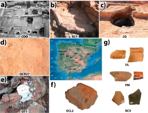
One of the main problems of the Iberian archeointensity database is the quality of the reported values, some-thing that affects not only the Iberian data but also the global paleointensity database (Genevey et al., 2008). According to the standard requirements in paleointensity studies (e.g., Genevey et al., 2008; Pavón-Carrasco, Gómez-Paccard, et al., 2014), 48% of the Iberian archeointensity data for the last three millennia can be regarded as high-quality data. Of this 48%, 81% are concentrated in the last two millennia (see Gómez-Paccard et al., 2016, for a review). For thefirst millennia BC, prior to Roman times, the majority of the data are based on one single specimen determination and they did not include the effects of the anisotropy of thermoremanent magnetization (ATRM) on archeointensity estimations. This important effect needs to be corrected at the specimen level (as it can be highly variable from specimen to specimen) for obtaining reliable paleointensity estimations. It can be particularly important for ceramics and tiles and can reach, in some cases, very high correction factors of more than 70% of the determinedfield strength (e.g., Chauvin et al., 2000; Genevey et al., 2008; Osete et al., 2016). Only three archeointensity data points fulfill the high-quality criteria for this time interval. In order to progress in the covering of the main gaps of the Iberian database, we have analyzed 247 samples from twelve archeological sites in Spain and 3 in Portugal. Their spatial distribution is shown in Figure 1. The age of the studied archeological sites ranges from the eleventh century BC to the nine-teenth century AD. Detailed information about the archeological context and sampling methods is available in supporting information Text S1 (Almagro-Gorbea & Álvarez-Sanchís, 1993; Álvarez-Sanchís et al., 2008;
Fernández Martínez et al., 1994; García i Rubert, 2015; García i Rubert et al., 2014; Garcia-Rubert et al., 2016; Gutiérrez Cuenca et al., 2016; López-Cachero, 2007; López-Cachero et al., 2008; Martín Viso et al., 2017; Molina & Salinas, 2013; Molina Expósito, 2004; Núñez, 2015; Proyecto Mauranus, 2011; Ruiz Zapatero, 2005; Salas Álvarez et al., 2014; Santos et al., 2012; Sastre Blanco, 2017; Thébault et al., 2015).
2. Magnetic Measurements
All the measurements were conducted in the paleomagnetism laboratories of Complutense University of Madrid (Spain) and University of Rennes 1 (France). Rock magnetic studies include a set of experiments in order to classify the magnetic carriers of remanence. Measurements include (i) hysteresis curves, (ii) acquisi-tion of isothermal remanent magnetizaacquisi-tion (IRM) curves, and (iii) subsequent direct current (DC) demagneti-zation (backfield IRM), all up to 500 mT. These three experiments were performed using a coercivity spectrometer (Jasonov et al., 1998). Some hysteresis loops were also obtained from a Petersen Instruments Magnetic Measurements Variable Field Translation Balance variablefield translation balance (with a maximum appliedfield of 1 T), (iv) Thermomagnetic curves: magnetic phase transitions such as Neel point and Curie tem-perature of magnetic carriers have been inferred from measurements of the lowfield susceptibility as a func-tion of temperature, heating up to 700 °C and further cooling to room temperature in an Ar atmosphere. The experiment has been carried out using a KLY-4S provided with a high-temperature furnace apparatus manu-factured by AGICO. Additional thermomagnetic curves were performed by a Petersen Instrument MMVFTB variablefield translation balance. Magnetization was measured in an applied field of 1 T, with heating and cooling carried out in air. (v) Thermal demagnetization of orthogonal IRMs was measured in selected samples from each site following the protocol outlined by Lowrie (1990). Magnetization of the specimen was achieved using 2 T along the sample Z axes, 0.6 T along the Y axes, and 0.2 T along the X axes. The magneticfield was applied using an ASC Scientific IM-10-30 Impulse Magnetizer. Samples were thermally demagnetized in MMTD80 or MMTDSC ovens manufactured by Magnetic Measurements, and magnetization measurements were made using a Minispin (manufactured by Molspin).
The Thellier demagnetization protocol including pTRM checks (Thellier & Thellier, 1959) was carried out for archeointensity determinations using MMTD80 or MMTDSC (Magnetic Measurements) ovens at Madrid and the Ramsès homemade ovens at Rennes. ATRM has been estimated at specimen level by determination of the ATRM ellipsoid following the method described by Veitch et al. (1984) and Chauvin et al. (2000). Figure 1. Locations of the studied archeological sites (center) and representative studied structures and sampling methods (a–g).
Stepwise thermal demagnetizations and alternatingfield demagnetizations were also conducted by means of the above-mentioned ovens and a GSD-5 alternating field tumbling demagnetizer (Schonstedt). Magnetization measurements were done using Minispin (Molspin) spinner magnetometers, JR5 (Agico) spin-ner magnetometers, or a superconducting magnetometer (2G). Low-field bulk susceptibility was measured after each step of thermal demagnetization using a KLY3 Kappabridge (Agico) or a Bartington MS3 suscept-ibility meter in order to detect magnetomineralogical alterations.
3. Results
3.1. Rock Magnetism
Representative samples from each site have been selected for rock magnetic analysis. Results here summar-ize the most common features found in a total of 150 analyzed samples including 91 hysteresis cycles and IRM acquisition and backfield IRM, 58 thermomagnetic curves, and 33 thermal demagnetizations of IRM cross components (Lowrie, 1990). Derived from each hysteresis loop, the saturation magnetization (Ms), saturation of remanent magnetization (Mr), and magnetic coercivity (Hc) have been computed after the subtraction of
the paramagnetic contribution (e.g., Evans & Heller, 2003). The following shows typical examples of rock mag-netic properties of characteristic materials in this study. Type I: small hearths with a thin burned surface (CAST, FER, SJ, PCR, QCR, GS, and EC1-EC4); type II: pottery kilns heated to high temperatures (RCV, COO, CSC, TO, and LQ), bricks (ECL and EC5) and ceramics (PM, UL, and RCV); type III: samples where a high coercivity com-ponent was present (some samples from COO and TO); and type IV: metallurgical kilns (OT).
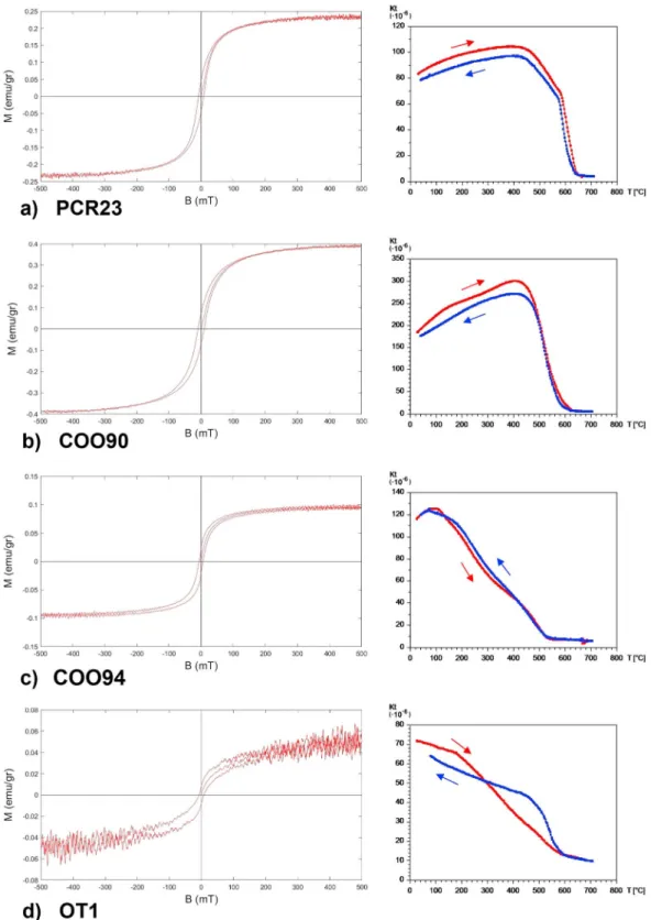
Magnetic hysteresis cycles from type I display closed hysteresis loops that saturate at about 150 mT and with coercivities about 5–10 mT (Figure 2a). This is compatible with magnetite/titanomagnetite. Samples from type II tend to have wider loops, with coercivities between 8 and 25 mT (Figure 2b), which is compatible with smaller grains of the same minerals, assuring a single domain (SD) or pseudo single domain (PSD) state that favors a better behavior during paleointensity experiments. Most of the investigated sites correspond to types I or II. Samples of type III have intermediate coercivities and slight wasp-waisted (goose-necked according to Tauxe et al., 1996) hysteresis loops (Figure 2c), suggesting the presence of two magnetic phases, a mixture of low-coercivity and high-coercivity phases (Tauxe et al., 1996). The wasp-waisted shape is clearer in some additional loops carried out up to 1 T in a MMVFTB (see supporting informa-tion Figure S1). The fourth category, type IV, contains some samples with similar features to type II, but others show a pronounced wasp-waisted shape (Figure 2d), suggesting the presence of two magnetic phases of different coercivities.
Experiments of IRM acquisition curves and subsequent backfield IRM from the same samples presented in the hysteresis experiments are summarized in the supporting information Figure S2. Samples from type I saturate atfields of about 150 mT. Backfield IRM curves allows computing Hcr, the coercivity of remanence, which is in the range of 15- to 25-mT samples from type II saturate atfields of about 200 mT, with an Hcrbetween 20 and
40 mT. This confirms the smaller domain size of particles of this category if the mineralogy is revealed to be equal in composition. Samples from Type III do not completely saturate at the maximum applied field (500 mT) but show a slight increase in the highfield magnetization after a sharp initial increase. Coercivity of remanence is higher than in previous categories, evidencing the contribution of a higher coercivity phase. These features are more pronounced in samples from type IV, which have wasp-waisted hysteresis loops, which are far from saturation at 500 mT and have coercivities of remanence that reaches up to 150 mT in some cases.
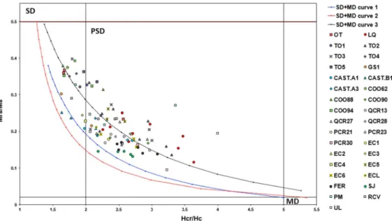
Magnetic parameters derived from hysteresis loops (Ms, Mr, and Hc) and backfield IRM (Hcr) can be
summarized in the named Day plot (Day et al., 1977; Dunlop, 2002). It classifies the domain state of magnetite/titanomagnetite bearing rocks, based on magnetization ratios (Mr/Ms) and coercivity ratios (Hcr/Hc). Results are summarized in Figure 3. Since Msand Hcrcan only be obtained from hysteresis loops that
reach saturation, nonsaturated samples have not been displayed. The majority of the represented samples are in the pseudo single-domain region and follow approximately the SD-MD mixing curves. Some points are shifted from the curves to the right, which mainly correspond to the EC5, COO, TO, and LQ structures, that is, type II materials. The more deviated points correspond to two ceramic samples that showed a wasp-waisted hysteresis loop. We want to note here that the use of the Day plot, especially for the interpretation of the domain state, should be carried out with care (see Roberts et al., 2018).
Figure 2. Hysteresis loops measured up to 500 mT (with initial magnetization curve) corrected for the paramagnetic con-tribution (left column) and thermomagnetic curves (right column) of representative samples. In thermomagnetic curves, red curve indicates the heating run and blue curve corresponds to the cooling experiment.
Based on thermomagnetic measurements, magnetic transition temperatures have been estimated in order to identify the magnetic carriers. A summary of thefindings is shown in Figure 2 (right panels). Samples from Type I display one magnetic transition in the range 550–580 °C suggesting the presence of magnetite/titanomagnetite with a low concentration of Ti. Some of them also show a transition at 630–650 °C, which could indicate the presence of maghemite. Type II samples present a single transition between 550 and 580 °C, which also indicates that magnetite/low-Ti content titatnomagnetite are the main minerals in these samples. Type III samples display two different magnetic transitions, one at about 200–300 °C and another at 560–580 °C. While the second one is the typical transition temperature for magnetite/titanomaghemite, the former is not as common and could be related to the low temperature phase already reported in archeomagnetic materials (McIntosh et al., 2007, 2011) recently identified as ε-Fe2O3(López-Sánchez et al., 2017). Type IV also show low temperature phase and the magnetite or titanoma-ghemite transition at 560–580 °C.
Complementary thermal demagnetization of IRM cross components was determined in selected samples. A summary is presented in supporting information Figure S3. Results confirm the presence of a low-coercivity phase (visible in the curves saturated at about 200 mT), which is the main carrier of magnetization in samples belonging to Type I and Type II. This phase loses its magnetization at temperatures between 550 and 600 °C, indicating the presence of magnetite/titanomagnetite of low Ti content. In samples from Type III a high-coercivity phase that is mainly demagnetized at about 200–300 °C is also observed, confirming the presence ofε-hematite (López-Sánchez et al., 2017). The low coercivity fraction is demagnetized after heating to 500–550 °C, consistent with the presence of magnetite or titanomagnetite/titanomaghemite with low Ti content. Type IV samples show a phase with high coercivity and low unblocking temperature, mainly demagnetized at 200 °C probably also associated withε-hematite. In the high-coercivity range, a small magnetization keeps demagnetizing until the maximum temperature, 600 °C, which can be due to the presence of hematite. Additionally, a low-coercivity component is also present. It demagnetizes with temperature up to 550–600 °C, when it is fully demagnetized, coherent with the presence of magnetite or titanomagnetite/titanomaghemite with low Ti content.
3.2. Archeomagnetic Directions
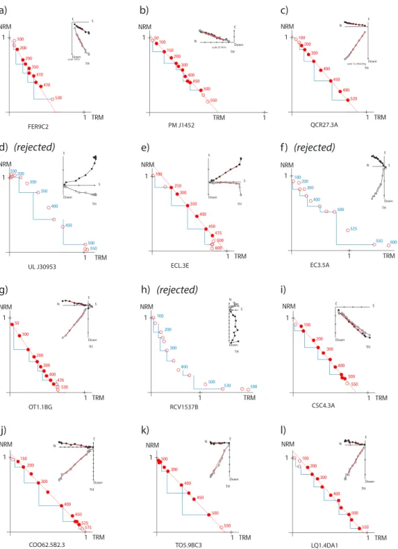
Most specimens presented a good magnetic behavior during alternating field (AF) and thermally (TH) demagnetization. After demagnetization of a small viscous component, which is usually fully removed at 100–150 °C or 5–10 mT and do not represent more than 15%–20% of the natural remanent magnetization (NRM), a single component that demagnetizes toward the origin is well isolated (Figure 4).
Figure 3. Dunlop-Day plot (Day et al., 1977; Dunlop, 2002) with representative samples. Samples from the same site are represented by the same color, but a different shape is used for each structure. SD-MD curves correspond to single-domain and multisingle-domain mixings presented by Dunlop (2002).
Only in a few sites two different components were found. These are the cases of the kilns from La Ferradura (FER) and San Jaume (SJ) and the tiles and some bricks reused for kiln construction in El Castillón (EC). In the case of tiles and the reused bricks (EC2.L4, EC5, and ECL) the component with higher unblocking temperature is likely related to its production, so no directional information of the past geomagneticfield can be obtained from that component. In contrast, the low-temperature component is related to the last heating of the com-bustion structure and has been used for directional calculations when the samples were oriented (see Figure 4c). In these cases, thefiring temperature could also be estimated.
The effect of thermoremanent anisotropy on mean directions from small andflattened thin kilns and hearths has been pointed out by Palencia-Ortas et al. (2017). They observed aflattening effect on the inclination up to 13°. In the kilns studied here, the effect of the ATRM on directions has been systematically investigated. It was found to be especially important in the EC site, where the ATRM correction for the inclination exceeds theα95
limit (see supporting information Table S1 and Table S2 for detail).
Directional results have been calculated by a linearfit of the characteristic component in Zijderveld plots (Zijderveld, 1967) and then corrected by the ATRM at specimen level. Table 1 presents directional mean direc-tions, and Figure 4 shows representative samples during thermal and AF demagnetization. Detailed informa-tion of direcinforma-tional results and the stereoplot for every structure can be found in supporting informainforma-tion Text S2 (Aitken & Hawley, 1971; Hus & Geeraerts, 1998, 2005; Saorin & Garcia i Rubert, 2016) and Figure S4, respectively.
3.3. Archeointensity Results
Intensity results were obtained by a linearfit in Arai plots (Nagata et al., 1963). The selected specimens showed positive pTRM checks, and its paleointensity was calculated with at least 5 points. Eighty percent of the selected specimens presented a fraction of the NRM used for slope determination, f> 0.6 (in any case, f> 0.4), 97% of the specimens had a quality factor, q > 10, and 88% presented maximum angular deviation and deviation angle below 5° (<6° in any case). Mean intensity results for every studied site are presented in Table 2 before and after the ATRM correction.
Figure 4. Representative Zijderveld diagrams fromstudied sites: (a) La Ferradura, (b) La Genestosa, (c) El Castillón, (d) Otero de Herreros, (e) Córdoba-Las Ollerías, (f) Córdoba-San Cayetano, (g) Toledo, and (h) Los Quemados. TH labels means thermally demagnetized specimens (step values are indicated in °C) and AF alternatingfield demagnetized (step values in mT).
CASTA structures are the oldest kilns studied. They correspond to small andflattened thin kilns that were pre-viously investigated for directional purposes by Palencia-Ortas et al. (2017). It was observed in this previous study that some alteration occurred after heating at 300–400 °C, which could make this site unsuited for paleointensity studies. However, the most external surface experienced much lower alteration. Therefore, specimens were subsampled and only small fragments (about 1 × 1 × 1 cm) from the external surface of the samples were prepared for the paleointensity experiments. This subsampling process increased notably the level of success of paleointensity protocols.
From CASTA3, high-quality linear NRM-TRM diagrams with successful pTRM checks were obtained from four of the six specimens investigated. The factor q was in some specimens near or over 100 (details in supporting information Table S3; Selkin & Tauxe, 2000). The last point retained for archeointensity determination was 400–450 °C, corresponding to the last temperature step before observing any evidence of changes in the mag-netic mineralogy or changes in the slop of Arai plot. ATRM correction was moderate and depended on the spe-cimen, with differences between the uncorrected and ATRM corrected paleointensity values that reached up to 11.4%. In three specimens a change in the slope of the Arai plot was observed at higher temperatures (after heating at 400 °C), also maintaining a linear trend. Paleointensities derived for this high-temperature compo-nent have also been calculated and compiled in Table S3. This high-temperature compocompo-nent could be attrib-uted to a chemical remanent magnetization (probably related to the chemical production of magnetite during the use of the kiln or alteration during laboratory treatment) and has not been considered further.
All specimens from CASTA1 were retained for the mean paleointensity calculation. High-quality linear NRM-TRM diagrams with successful pNRM-TRM checks were observed in all specimens investigated. Accurate determi-nation of the past paleofield was obtained (53.1 ± 3.1 μT).
Most FER samples showed an important viscous component up 300–350 °C and curved Arai plots, which make them unsuited for intensity studies. Only 7 from the 22 studied specimens, from which the low-Table 1
New Directional Data From This Study
Site Latitude (°N) Longitude (°E) Age Dating method N n nrej Da (deg) Ia (deg) ka α95 a (deg) DM (deg) IM (deg) FER 40.60 0.50 650 ± 100 Arch 17 17 5 19.8 61.5 175 2.7 19.7 60.4 SJ 40.57 0.52 650 ± 100 Arch 0 0 20 — — — — — — GS2 40.35 6.77 150 ± 75 Arch 8 8 3 4.1 57.9 359 2.9 4.2 58.1 EC1i 41.84 5.79 525 ± 25 Arch 11 12 0 9.6 56.6 104 4.3 9.6 55.5 EC1s 41.84 5.79 525 ± 25 Arch 7 10 0 4.9 62.2 331 2.7 4.7 61.1 EC2 41.84 5.79 525 ± 25 Arch 8 19 0 0.8 57.9 243 2.2 0.6 56.5 EC5 41.84 5.79 525 ± 25 Arch, C14 1 5 8 3.5 59.1 621 3.1 3.5 57.9 OT 40.82 4.22 529 ± 86 TL 3 22 1 2.0 59.3 333 1.7 2.0 58.9 EC3+4 41.84 5.79 550 ± 50 Arch 5 17 6 3.1 63.9 215 2.4 3.2 62.7 COO90 37.88 4.77 950 ± 50 Arch 8 8 0 20.5 54.6 1607 1.4 21.3 57.2 CSC4 37.89 4.77 1000 ± 50 Arch 3 8 1 18.8 38.9 113 5.2 19.5 42.5 CSC3 37.89 4.77 1150 ± 50 Arch 3 7 2 17.7 37.5 169 4.7 18.4 41.2 COO62 37.88 4.77 1200 ± 100 Arch 8 8 0 14.1 42.1 376 2.9 14.7 45.5 COO88 37.88 4.77 1200 ± 100 Arch 6 6 0 11.2 41.0 156 5.4 11.7 44.5 COO94 37.88 4.77 1200 ± 100 Arch 7 7 1 6.7 39.8 643 2.2 7.1 43.3 CSC1 37.89 4.77 1225 ± 25 Arch 7 12 2 6.7 38.7 604 1.8 7.2 42.3 CSC2 37.89 4.77 1225 ± 25 Arch 6 10 2 11.0 38.4 302 2.8 11.5 42.0 TO4 39.86 4.03 1676 ± 29 Amag 8 8 0 0.1 66.3 516 2.4 0.0 66.7 TO3 39.86 4.03 1788 ± 22 Amag 7 14 4 21.9 65.2 437 1.9 22.2 65.5 TO2 39.86 4.03 1816 ± 36 Amag 8 8 2 25.1 63.5 355 2.9 25.4 63.8 TO1 39.86 4.03 1807 ± 21 Amag 2 6 3 23.1 63.5 1576 1.7 23.3 63.8 TO5 39.86 4.03 1822 ± 56 Amag 10 10 0 17.9 62.0 382 2.5 18.1 62.4 EC6 41.84 5.79 629 ± 86/1644 ± 67 Amag 5 7 9 7.5 66.0 113 5.7 7.0 65.1 LQ 39.43 2.63 1439 ± 17 Amag 10 33 6 9.2 48.4 298 1.5 9.1 49.4 Note. Site, name of the studied structure; latitude, longitude, coordinates of the structure; age (years), assigned age; dating method, dating method (C14, radio-carbon; Arch, archeological constraints; Amag, archeomagnetism); N, number of independent samples included in mean calculation; n, number of specimens retained for mean calculation; nrejnumber of specimens rejected; D, site mean declination; I, site mean inclination; k, precision parameter;α95, semiangle of
95% confidence limit; DM, mean declination relocated to Madrid; IM, mean inclination relocated to Madrid. Subindex a indicates values after ATRM correction
temperature component is less important, have given a passable result (Figure 5a). Results from SJ, a contemporaneous site from the same archeological complex as FER, were noisy, curved and thus, unsuited for either directional or intensity calculations. The site has been rejected. Arai plots from some PM ceramic samples are quite noisy (Figure 5b) but provide intensities consistent with the FER kiln, a probably contemporaneous site located about 400 km away from Pedro Muñoz site. Only four specimens passed the considered quality criteria and provided one intensity result (Table 2). As expected for ceramic materials, ATRM corrections are not negligible; nevertheless, they are not very high in this case, with values ranging between 3.5% and 9.7%.
Portuguese sites of the First Iron Age (PCR, QCR, and CASTB) showed a single component that demagnetizes towar the origin and provided good linear Arai plots allowing the calculation of archeointensities from 100– 150 °C to 400–500 °C (Figure 5c). The ATRM corrections are quite variable throughout the different structures, Table 2
New Archeointensities From This Study
Site Latitude Longitude Age Dating method n nrej F ±σF Fa±σFa Fa Mad VADM
CASTA3l 41.22 6.95 1,100 ± 200 TL 4 2 71.7 ± 3.5 66.4 ± 4.3 65.7 ± 4.3 113.2 CASTA1 41.22 6.95 900 ± 200 TL 4 0 57.3 ± 4.4 53.1 ± 3.1 52.6 ± 3.1 90.5 FER 40.60 0.50 650 ± 100 Arch 6 16 80.7 ± 7.3 83.8 ± 6.5 83.6 ± 6.5 143.8 SJ 40.57 0.52 650 ± 100 Arch 0 30 — — — — PM 39.41 2.95 500 ± 50 Arch 5 4 82.1 ± 8.9 87.2 ± 8.1 88.2 ± 8.1 151.7 PCR23 41.26 6.86 300 ± 150 TL 6 0 65.4 ± 11.6 58.4 ± 3.9 57.8 ± 3.9 99.5 PCR21 41.26 6.86 293 ± 93 C14 4 2 59.1 ± 4.1 55.8 ± 3.7 55.2 ± 3.7 95.0 QCR27 41.26 6.86 275 ± 85 C14 6 0 60.2 ± 2.2 58.1 ± 3.6 57.5 ± 3.6 99.0 CASTB1 41.22 6.95 190 ± 150 TL 6 0 61.5 ± 6.9 59.3 ± 3.3 58.7 ± 3.3 101.1 QCR13 41.26 6.86 170 ± 120 TL 5 1 57.3 ± 2.2 54.3 ± 1.9 53.7 ± 1.9 92.5 UL 40.55 4.90 100 ± 50 Arch 4 6 — — — — QCR28 41.26 6.86 60 ± 130 TL 4 2 66.4 ± 11.2 65.9 ± 2.2 65.2 ± 2.2 112.3 PCR17 41.26 6.86 28 ± 78 C14 0 2 — — — — PCR30 41.26 6.86 30 ± 100 TL 6 0 56.6 ± 8.5 59.3 ± 3.3 58.7 ± 3.3 101.0 GS2 40.35 6.77 150 ± 75 Arch 4 7 69.0 ± 3.1 68.0 ± 3.6 68.0 ± 3.6 117.0 ECLh 41.84 5.79 475 ± 25 Arch 5 12 63.6 ± 2.5 54.3 ± 0.9 53.4 ± 0.9 91.9 EC1i 41.84 5.79 525 ± 25 Arch 4 2 52.0 ± 6.5 49.9 ± 5.8 49.1 ± 5.8 84.4 EC1s 41.84 5.79 525 ± 25 Arch 4 1 60.7 ± 1.8 56.0 ± 2.9 55.1 ± 2.9 94.8 EC2 41.84 5.79 525 ± 25 Arch 4 6 55.0 ± 10.3 52.7 ± 9.9 51.8 ± 9.9 89.2 EC5 41.84 5.79 525 ± 25 Arch, C14 4 9 67.8 ± 4.3 57.9 ± 3.3 56.9 ± 3.3 98.0 OT 40.82 4.22 529 ± 86 TL 10 0 61.2 ± 6.2 64.0 ± 7.3 63.7 ± 7.3 109.6 EC3-4 41.84 5.79 550 ± 50 Arch 4 6 65.2 ± 5.0 61.5 ± 4.6 60.5 ± 4.6 104.1 GS1 40.35 6.79 600 ± 100 Arch 0 6 — — — — RCV 43.40 3.70 700 ± 100 Arch 0 7 — — — — COO90 37.89 4.77 950 ± 50 Arch 4 4 51.4 ± 5.9 51.5 ± 6.6 53.0 ± 6.6 91.2 CSC4 37.89 4.77 1,000 ± 50 Arch 6 0 58.7 ± 3.3 58.1 ± 3.7 59.8 ± 3.7 102.9 CSC3 37.89 4.77 1,150 ± 50 Arch 5 1 68.2 ± 5.8 63.5 ± 4.3 65.4 ± 4.3 112.5 COO62 37.89 4.77 1,200 ± 100 Arch 8 0 52.7 ± 4.5 53.4 ± 4.5 55.0 ± 4.5 94.6 COO88 37.89 4.77 1,200 ± 100 Arch 6 0 50.1 ± 4.0 49.2 ± 2.7 50.6 ± 2.7 87.1 COO94 37.89 4.77 1,200 ± 100 Arch 6 2 50.3 ± 3.5 50.4 ± 2.0 51.9 ± 2.0 89.3 CSC1 37.89 4.77 1,225 ± 25 Arch 5 1 56.9 ± 4.8 56.5 ± 2.4 58.1 ± 2.4 100.1 CSC2 37.89 4.77 1,225 ± 25 Arch 6 0 53.3 ± 3.7 52.0 ± 5.5 53.5 ± 5.5 92.1 TO4 39.86 4.03 1,676 ± 29 Amag 5 3 52.8 ± 1.9 53.5 ± 1.7 53.8 ± 1.7 92.6 TO3 39.86 4.03 1,788 ± 22 Amag 11 0 53.4 ± 5.3 52.7 ± 5.7 53.0 ± 5.7 91.2 TO2 39.86 4.03 1,816 ± 36 Amag 4 6 54.2 ± 2.2 51.8 ± 2.2 52.1 ± 2.2 89.7 TO1 39.86 4.03 1,807 ± 21 Amag 5 4 48.7 ± 1.9 47.8 ± 1.2 48.1 ± 1.2 82.7 TO5 39.86 4.03 1,822 ± 56 Amag 10 0 48.3 ± 4.0 48.5 ± 3.2 48.8 ± 3.2 83.9 EC6 41.84 5.79 629 ± 86/1,644 ± 67 Amag 0 30 — — — — LQ 39.43 2.63 1,439 ± 17 Amag 11 4 49.5 ± 3.0 49.0 ± 3.1 49.5 ± 3.1 85.2 Note. Site, name of the structure from which the material was recovered; latitude (°N), longitude (°E), coordinates of the investigated site; Age (years), assigned age; dating method, dating method used for age assignment (TL, thermoluminescence; C14, radiocarbon; Arch, archaeological constraints; Amag, archaeomagnetic dating); n, number of specimens retained for mean calculation; nrejnumber of specimens rejected; F ±σF(μT), mean intensity and standard deviation before
ther-moremanent magnetization (TRM) anisotropy correction; Fa±σFa(μT), mean intensity and standard deviation corrected for TRM anisotropy; Fa Mad(μT), mean
anisotropy of TRM-corrected intensity relocated to Madrid; VADM (ZAm2), value of the virtual axial dipole moment. Indices: l, component of low unblocking tem-perature; and h, component of high unblocking temperature.
samples, and even between different specimens from one sample, confirming the need to perform the ATRM correction at the specimen level. ATRM correction ranged up to 34.2% at specimen level. The PCR17 pilot sample showed a curved Arai plot. Since this behavior is not suitable for paleointensity determination, the structure was rejected and no more samples were analyzed.
Figure 5. Representative Arai plots from studied sites: (a) La Ferradura, (b) Pedro Muñoz, (c) Quinta de Crestelos, (d) Ulaca, (e, f) El Castillón, (g) Otero de Herreros, (h) Ríocueva, (i) Córdoba-San Cayetano, (j) Córdoba-Las Ollerías, (k) Toledo, and (l) Los Quemados. Filled circles represent the chosen interval for paleointensity calculations. A small Zijderveld plot of each selected specimen is also represented showing the NRM structure.
Ceramic samples from Ulaca site provided quite noisy Arai plots, and some of them presented two compo-nents, indicating that some fragments were reheated at least two times. The majority also presented high maximum angular deviation and deviation angle values (Figure 5d), and we have rejected the site. Although we have not considered any quality result from this site, a mean intensity could be derived from a few specimens (Table S4), with results consistent with the values obtained from the Portuguese kilns and hearths of similar age. ATRM corrections were important, with values up to 75.6%.
Results from GS2 provided linear Arai plots from which consistent values of paleointensity have been obtained between 100 °C and 440 °C. The ATRM correction was small, less than 1.5%.
Structures from El Castillón (EC1–EC5) have allowed the calculation of five new archeointensity data. An addi-tional value has been calculated from the high-temperature component of the ECL3 brick (250–475 °C; Figure 5e). ATRM corrections ranged from 0.7% to 10.6% in EC1-EC4 structures and higher, between 11.1% and 17.7%, in the bricks samples (EC5 and ECL3). Other unoriented bricks have been rejected because of alteration during Thellier-Thellier experiments (ECL1) or the presence of two overlapping components (ECL2). Curved Arai plots were obtained from all EC6 specimens. Thermomagnetic curves demonstrated the presence of very unstable phases that alter even at temperatures as low as 200 °C. The EC6 site has con-sequently been discarded.
The Thellier-Thellier protocol has been applied to some specimens from OT1 samples and some unoriented fragments of OT4floor. Satisfactory results have been obtained, finding a single component and straight Arai plots with no evidence of important alteration (Figure 5g). ATRM corrections were low (between 0.5% and 8.8%) except for two specimens having higher corrections (17% and 19.5%).
Arai plots from the GS1 site presented two linear segments. We have no archeological or rock-magnetic criteria to keep the high- or the temperature paleointensity determination. The low-temperature component provides high intensities that could be in agreement with the high paleofield values reported around 600 AD and 800 AD (Gómez-Paccard et al., 2012). However, the statistical para-meters do not fit our selection criteria and the derived paleointensities have not been considered. In contrast, the high-temperature component is well defined and the statistical parameters analyzed meet the selection criteria. The derived paleointensity is 49.0 ± 2.3 μT. As we do not have a convincing explanation, apart from statistical reasons, to maintain this result, we have preferred to be cautious and not to include this result in the Iberian database. It is included in the supporting information Table S4.
Ceramics from RCV were rejected. Several overlapping components were observed that produced curved Arai plots (Figure 5h). Furthermore, all thermomagnetic curves of specimens from this site showed the pre-sence of unstable phases that undergo alteration during heating.
The Córdoba sites provided good archeointensity results with characteristic components isolated from 100 to 500 °C (CSC; Figure 5i) or between 100–250 and 400–525 °C (COO; Figure 5j). Above these temperatures, some alteration is sometimes observed, but thermomagnetic curves show an overall stable behavior. Obtained means are quite accurate with an error between 2 and 3μT after the ATRM correction at specimen level, which is between 0.0% and 15.1% in CSC and between 0.0% and 9.3% in COO.
The ceramic kilns from Toledo (TO) supply good Arai plots (Figure 5k). No evidence of alteration has been found until the highest-temperature steps. Very accurate paleointensities have been obtained for the TO1, TO2, and TO4 structures, with errors between 1.2 and 2.2μT. Except for a few specimens, the ATRM is less than 5%.
Good paleointensity estimations have also been derived from the LQ site. A single component, isolated between 50–200 °C and 500–550 °C, trended toward the origin and provided linear Arai plots (Figure 5l). No age information could be obtained from the urgent archeological exploration. The full vector derived for the archeomagnetic study has been used for dating this site.
In summary, from the 367 specimens analyzed in this work, 191 have been retained and used for calculating 34 new high-quality paleointensities for Iberia. Twenty-seven of them have nonarcheomagnetic datings and are suitable for PSVC construction.
4. The First Full-Vector Iberian Paleosecular Variation Curve for the Last
Three Millennia
4.1. Revisiting the Iberian Database for the Last Three Millennia
Since thefirst Iberian catalogue was published in 2006 (Gómez-Paccard, Catanzariti, et al., 2006), numerous archeomagnetic studies have complemented the existing temporal gaps and improved the spatial distribu-tion of the database (supporting informadistribu-tion Figure S5). This work increases the number of high-quality direc-tions by 14%, up to 132, and the number of high-quality archeointensities by 59%, up to 73 data. Especially important is the increase of archeointensities for thefirst millennium BC, providing 11 new quality data when there were only three (Osete et al., 2016). Thefinal database is available in supporting information Table S5.
4.2. Generating a New PSVC for Iberia
The new PSVC for Iberia has been centered in Madrid (40.4°N, 3.7°W) and includes all high-quality archeo-magnetic data from the reviewed GEOMAGIA50.v3.2 database (Brown et al., 2015) within a radius of 900 km. This means that data coming from northern Morocco and southern France have also been consid-ered to complete the Iberian catalogue. The following statistical criteria have been used to select the high-quality archeomagnetic data: (1) age error≤250 years, (2) number of specimens used to obtain the mean value presented in the database≥4, (3) α95≤ 5.0°, and (4) paleointensities must be obtained by the original
or derived Thellier-Thellier method with pTRM checks, with TRM anisotropy correction if derived from poten-tial high-anisotropic objects (such as potteries, ceramics, and pipes). This criterion was especially restrictive for paleointensities, since only 52% of the studies passed the selection requirements.
The archeomagnetic database for the last three millennia contains 523 high-quality data (204 declinations, 204 inclinations, and 115 intensities), which have been relocated to Madrid coordinates using the virtual geo-magnetic pole method (Noël & Batt, 1990). Seven additional available high-quality data between 1300 BC and 1000 BC (three declinations, three inclinations, and one intensity) have also been considered in order to mini-mize edge effects in oldest ages when computing the PSVC. For the most recent times, we introduced also directional and intensity historical data coming from the HISTMAG database (Arneitz et al., 2017) including 1101 declinations, 162 inclinations, and 164 intensities.
In order to obtain a time-continuous full vector PSVC, we have taken into account the intrinsic relations between the three elements of the geomagneticfield (i.e. declination D, inclination I, and intensity F) consid-ering all of them together. For this, we reconstruct the past temporal evolution of the geomagneticfield at a reference point P (θ, λ) at the Earth’s surface, by defining a full-vector M of the geomagnetic field at that point assuming a dipole vector (equations S1 and S2 in supporting information Text S3). The time evolution is represented by cubic b-splines with knot points every 50 years. Afirst PSVC is obtained to check and reject possible outliers (13 archeomagnetic data were discarded). Next, thefinal PSVC is calculated. The error of thefinal PSVC is determined by a bootstrap approach in which the available stratigraphical information is taken into account. The methodology used to develop the PSVC is explained in detail in the supporting infor-mation Text S3 (De Boor, 2001; Hellio et al., 2014; Lanos, 2004; Lanos et al., 2005; Thébault & Gallet, 2010).
4.3. The PSVC for Iberia
The obtained full vector Iberian PSVC for the last three millennia is shown in Figure 6. The new directional results from this work agree with previously available data. The evolution of declination (Figure 6a) is charac-terized by a maximum value of deviation to the east of 22° around 800 BC followed by a decrease until 400 BC, when the Earth’s magnetic field exhibited northern directions that are maintained for about eight centu-ries with no significant variations. Then, declination increases between 400 AD and 700 AD up to a value of 15° in seventh to twelfth centuries. The new obtained data from sixth century AD help to better define the start of the eastern declinations. At 1600 AD an important westward drift started until the end of the curve in 1900 AD. Inclinations presented three maxima, reaching about 60°–65° at 500 BC, 600 AD, and 1700 AD, intercalated by two minima, one at 200 AD with a value around 53° and the other at 1400 AD with an inclina-tion of about 45° (Figure 6c).
The most important contribution of this work is related to the intensity component. The curve presented in Figure 6e is thefirst intensity curve for Iberia. The two new data coming from two independent sites (the kiln from FER and ceramic fragments from PM) helped to reveal a significant maximum around 600 BC, with
intensity values reaching 85μT, the highest intensities observed in the Iberian Peninsula in the last three millennia (Figure 6e). Small variations around a mean value of 60μT are observed between 400 BC and 500 AD with a small maximum around 100 AD. A second maximum is evidenced betweenfifth and ninth centuries AD, reaching a value of 70μT at 800 AD. After that, a slow decrease in intensity is observed.
5. Discussion
5.1. The New PSVC: Application to Archeomagnetic Dating
The new PSVC will be useful for archeomagnetic dating in the Iberian Peninsula, since it has been developed with all the currently available high-quality data from the region. Furthermore, the new curve contains infor-mation on the full geomagnetic vector variations, that is, declination, inclination and intensity, which allows improving the accuracy of dating by using all of the three components.
Seven studied structures, for which there was not enough information about their chronology, have been archeomagnetically dated using the new PSVC by means of the archeo_dating program (Pavón-Carrasco et al., 2011). Figures depicting the dating results are available in supporting information Figure S7. The hearth EC6 has been dated based on its direction, providing two possible periods: 629 ± 86 AD or 1644 ± 67 AD, Figure 6. New Iberian PSVC together with the data used for its construction (a, c, and e) and compared with other curves and regional and global models (b, d, and f). Every curve has been represented with a 2-sigma error band. Open circles represent the outliers rejected for curve calculation.
together with another period (455 ± 223 BC) that should be clearly discarded by the archeological context. On the other hand, the big lime kiln from LQ has been dated using all three magnetic components, resulting in an age of 1439 ± 17 AD. Thefive TO kilns have been dated using their directions and intensities, providing ages consistent with the suspected ones. The obtained ages were for TO1, 1807 ± 21 AD; for TO2, 1816 ± 36 AD; for TO3, 1788 ± 22 AD; for TO4, 1676 ± 29; and for TO5, 1822 ± 56 AD. This means that TO4 is the oldest, while the others have approximately the same age.
5.2. Comparison With Other Western European PSVCs
The new curve has been compared with other local and model-derived PSVCs in Figure 6 (right): the Iberian PSVC centered in Madrid Paccard, Lanos, et al., 2006), the French curves centered in Paris (Gómez-Paccard et al., 2016; Hervé et al., 2013a, 2017) and relocated to Madrid coordinates, and the model predictions derived from the regional models SCHA.DIF.3k (Carrasco et al., 2009) and model B from Pavón-Carrasco, Gómez-Paccard, et al. (2014) and the last global model (HFM.OL1.A1, Constable et al., 2016) com-puted for Madrid coordinates. A general agreement is observed in directions (with the exception of the glo-bal HFM.OL1.A1), but some differences in paleointensities are evidenced.
The directional PSVC by Hervé et al. (2013a) for Paris is in agreement with our curve in all its interval of validity. Directional components of our PSVC and the previous Iberian curve proposed by Gómez-Paccard, Lanos, et al., 2006 are very similar as well (Figures 6b and 6d). Small differences (less than 5°) appear in the declina-tion maximum in 900 AD and minimum in 1800 AD and in the inclinadeclina-tion maximum in 1700 AD. This is not surprising since in 2006 there was barely any data for those periods in the region (Gómez-Paccard, Lanos, et al. (2006). The new directional curve is also in general agreement with the predictions from the regional model SCHA.DIF.3k (Pavón-Carrasco et al., 2009), except for the 1600–1800 AD period where lower inclina-tions are predicted by the Iberian PSVC. Significant differences for the first millennium BC are observed between the curve derived from the HFM.OL1.A1global model, the new Iberian curve, and the regional and local curves.
PSVCs for intensity in Paris (Gómez-Paccard et al., 2016; Hervé et al., 2017) show a good agreement with our paleointensity curve, although it is important to indicate that the Iberian curve is smoother than the French ones. This is probably because it includes a smaller amount of data. The main difference is the amplitude of the minimum at 800 BC, just before the high maximum observed at 600 BC and the absence of a double max-imum at the 600–800 AD interval. The Iberian paleointensity curve does not have any trace of the 600 AD maxima, which is clearly observed in the eastern European database (Genevey et al., 2003) and recently sug-gested by French data (Gómez-Paccard et al., 2012). More archeomagnetic information is still needed to obtain a more detailed description of the paleofield in the Iberian region and to understand the nature of this double maxima.
Major differences are observed in paleointensities with the SCHA.DIF.3k regional model (Pavón-Carrasco et al., 2009). These differences are due to the input databases. In the construction of the regional SCHA. DIF.3k model, no quality requirements related to the laboratory protocol were considered and, on another hand, all the data from Europe contributed to the expected values in Iberia. For example, it is important to notice that for thefirst millennium BC, only few intensity data from Western Europe were published when the SCHA.DIF.3k model was constructed. It means that the model was mostly based on the eastern European paleointensity database. In a more recent regional reconstruction (pink curve in Figure 6f) provided by Pavón-Carrasco, Gómez-Paccard, et al. (2014), quality requirements were included for paleointensities similar to the ones used here. In spite of the differences in shorter wavelengths, the general trend is more consistent. For thefirst millennia BC, the regional reconstruction by Pavón-Carrasco, Gómez-Paccard, et al. (2014) shows a maximum of comparable intensity value at about 600 BC, but the secondary maxima observed at ~900 BC is not registered by the Iberian PSVC. For the last two millennia, the European recon-struction indicates a high maximum around 600 AD that it is not observed in the Iberian PSVC but it is sug-gested, although of lower intensity, in the western European PSVC by Gómez-Paccard et al. (2016). It is important to notice that when a regional or global reconstruction is performed, the spatial resolution is limited by the amount of data, its distribution, the internal consistency of the database, and the harmonic expansion degree used in the modelling process. That is, for example, the eastern European database con-trolled most of paleointensity predictions derived from the SCHA.DIF.3k model. The most recent
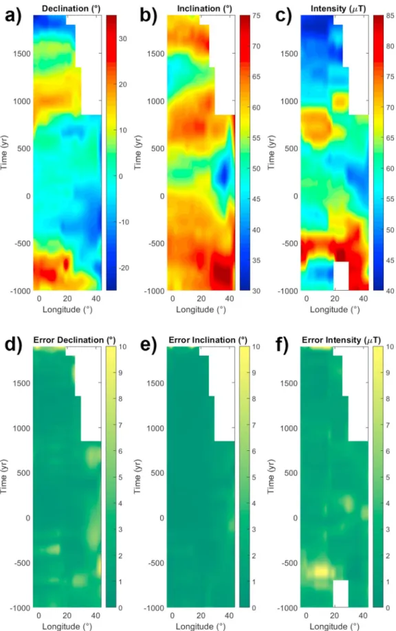
Figure 7. Hovmöller diagrams for declination (a), inclination (b) and intensity (c), and their uncertainty (d–f) through Europe and the Middle East reduced to the lati-tude of Madrid (see text for details). White areas indicate that no quality data are available for that curve and period.
reconstruction of Pavón-Carrasco, Gómez-Paccard, et al. (2014) was only based on high-quality paleointensity data. That is, it was based on a much smaller number of data. As a consequence, few data seems to have a high influence on the model. To investigate more in detail variations of the secular variation at continental scale, we have followed an innovative approach that is presented in next section.
5.3. The Secular Variation in the Mediterranean Region for the Last 3,000 Years
We have calculated several PSVCs starting with the new Iberian PSVC and continuing through Europe and Middle East following the zones with more available data (see supporting information Figure S8) in order to calculate the most accurate PSVCs possible. For each point, a PSVC has been computed using all quality data within a radius of 900 km following the same methodology (supporting information Text S3). Then, they have been relocated to the latitude of Madrid without varying its longitude. The resulting curves are available in supporting information Figure S9. All the curves have been resumed in a so-called Hovmöller diagram (Hovmoller, 1949) for each component. In these diagrams, the declination, inclination or intensity, as well as their errors, have been mapped in colors in function of longitude and time (Figure 7). This representation allows us to investigate more in detail the evolution of the paleofield in space and time in an east-west direc-tion around the Mediterranean region.
The most remarkable feature of the past secular variation in thefirst half of the first millennium BC is the high intensities, of about 80μT, observed at longitudes between 30 and 40°E (Figure 7c). At 1000 BC the maximum is centered at 35°E, which is related to the Levantine Iron Age Anomaly (LIAA) proposed by Shaar et al. (2016, 2017). This is an unusual feature of the Earth’s magnetic field, also known as geomagnetic intensity spikes (Ben-Yosef et al., 2009), which is characterized by very highfield intensity values associated with rapid secular variation rates. High-intensity values potentially related to spikes have recently been reported from the Canary Islands (de Groot et al., 2015; Kissel et al., 2015) and eastern China (Cai et al., 2017). The existence of geomagnetic spikes has produced a great interest and debate (e.g., Davies & Constable, 2017; Korte & Constable, 2018; Livermore et al., 2014). Livermore et al. (2014) considered that the reported rates of secular variation from the LIAA were not compatible with the commonly accepted core-flow dynamics hypothesis. Davies and Constable (2017) proposed that the Levantine spike could be caused by a narrow localized intenseflux patch at the core-mantle boundary, first growing in place and then migrating north and west-ward. Very recently, Korte and Constable (2018) suggested that the spikes are originated from intenseflux patches growing and decaying mostly in situ, combined with stronger and more variable dipole moment than shown by previous globalfield models.
The 1000 BC maximum is observed later, at 700 BC, between 20° E and 25 °E. From the analysis of Figure 7c it seems that both maxima could be related to the same feature moving westward. Following that idea, it could correspond also to the intensity maximum in Iberia we have reported at 600 BC. It is noticeable that between 0° and 20°E lower intensities appear at 500 BC, but it should be pointed out that the curves were calculated for points centered in latitudes further north (see supporting information Figure S8) and later translated to Madrid latitude for comparison. That would indicate that if the LIAA was a moving anomaly, it would have travelled by latitudes below 45°N. In addition, the error is also higher in that period (Figure 7f). Moreover, it is important to note that a peak infield strength around 600 BC has also been suggested from the Canary Islands (de Groot et al., 2015; Kissel et al., 2015) and from the Azores Archipelago (di Chiara et al., 2014), sug-gesting the possibility of a larger scale intensity maximum. More data are needed in order to have a clearer view of the extension of this feature.
The movement of that intensity anomaly could also have had some effect on directional components and, in fact, it seems related to high inclinations values and eastern declinations (Figures 7a and 7b). The maximum in inclination is observed between 30° and 40°E longitudes at 800 BC. It moved westward, reaching 0° long-itudes at around 500 BC. Eastern declinations seem to be related to the anomalous high intensity values, although the Hovmöller diagrams do not show a clear displacement of the patch. To assess if this behavior could be due to geomagnetic pole drift or dipole intensity variations, we have built also Hovmöller diagrams with synthetic curves from the dipole (n = 1) component and for the fullfield components of the SHA.DIF.14k model (Pavón-Carrasco, Osete, et al., 2014) and the ARCH10k1 model (Constable et al., 2016; supporting information Figure S10 and Figure S11). According to these representations, the dipole cannot explain the intensity values or the directional changes. This feature should be ascribed to higher degrees of the harmonic decomposition according to the global models used. However, Korte and Constable (2018) considered that
the current global database distribution prevents the description of such features by available spherical har-monic models (see supporting information Figures S10b and S11b). In this context, simple representations such as those proposed here through the Hovmöller diagrams can be of great interest.
After the LIAA maximum, a low in intensity moving westward is observed at 100 AD around 40°E longitudes. This low in intensity vanishes as it moves westward, reaching the longitude of 0°E at 500 AD.
Another feature worth highlighting is the double oscillation in intensity at 600 AD and 800 AD observed in some European regions. We have discussed above that despite the fact that other curves and models present the double maximum, our new PSVC does not. In Figure 7c, the double oscillation is only clear for the curves of longitudes between 0°E and 15°E, which makes us wonder if it could also be a matter of latitude, explaining why it could be registered in northern France and not in Iberia. Since currently there is hardly any data at higher or lower latitudes in Western Europe, this question cannot be answered for the moment.
Another clear characteristic is observed in the Hovmöller diagrams between 500 AD and 1000 AD. In this case, it is a feature that moves eastward and evidenced in the directional components of the paleofield. It is observed as a shifting maximum in inclination and a drift in the 0° declination line (Figures 17a and 17b). This feature is mainly due to the geomagnetic dipole passing through these longitudes (see supporting information Figure S12), increasing inclination and making declination tend to 0° at the longitude where the pole is. Supporting information Figures S10a and S11a show that the dipole represents well this feature. Finally, we would like to point out the potential of the Hovmöller diagrams in investigating drifting features of the magnetic paleofield, a tool that is seldom used in archeomagnetism, although the use of time-longitude plots have been used in mapping core-mantle-boundaryfield structure (e.g., Korte & Constable, 2018; Nilsson et al., 2014). This kind of diagram can help us identifying small wavelength spatial features of the geomag-neticfield, which are probably more difficult to analyze from regional or global modelling. However, in this type of analysis, we must take care with the relocation errors that occur when data or curves are transported (e.g., Casas & Incoronato, 2007; Pavón-Carrasco et al., 2011). Nevertheless, prior to the use of any analysis technique, it is still important to increase the number of archeomagnetic data even in regions, such as Europe, which have the highest density of archeomagnetic data.
6. Conclusions
We have presented 16 new directional and 27 new archeointensity quality data from Iberian sites, incorpor-ating them to the Iberian archeomagnetic database and covering some spatial and temporal gaps in it. Then, a new full-vector PSVC centered at Madrid have been constructed and compared with other PSVCs and mod-els. The most important point showed by the new curve is the existence of a high intensity maximum around 600 BC. The absence of the double intensity oscillation in 600–800 AD recorded in other European curves, and models should also be highlighted.
The joint analysis of European data suggest that the Levantine Iron Age Anomaly could be envisaged as a local magnetic paleofield feature drifting westward. Whether geomagnetic intensity spikes can move or are static is a current and important debate (Davies & Constable, 2017; Korte & Constable, 2018). The Hovmöller diagram has proved useful in analyzing this kind of small wavelength feature, which are not well represented by current models. More data are still needed to better constraint its spatiotemporal evolution.
References
Aitken, M. J. (1970). Dating by archaeomagnetic and thermoluminescent methods. Philosophical Transactions of the Royal Society A, 269, 1193. https://doi.org/10.1098/rsta.1970.0087
Aitken, M. J., & Hawley, H. N. (1971). Archeomagnetism: Evidence for magnetic refraction in kiln structures. Archeometry, 13, 83–85. Almagro-Gorbea, M., & Álvarez-Sanchís, J. R. (1993). La sauna de Ulaca. Saunas y baños iniciáticos en el mundo céltico. Cuadernos de
arqueología de la Universidad de Navarra, 1, 177–232.
Álvarez-Sanchís, J. R., Marín, C., Falquina, A., & Ruiz Zapatero, G. (2008). El oppidum vettón de Ulaca (Solosancho, Ávila) y su necrópolis. In J. R. Álvarez-Sanchís (Ed.), Arqueología Vettona. La Meseta Occidental en la Edad del Hierro, Zona Arqueológica (Vol. 12, pp. 338–361). Alcalá de Henares: Museo Arqueológico Regional.
Arneitz, P., Leonhardt, R., Schnepp, E., Heilig, B., Mayrhofer, F., Kovacs, P., et al. (2017). The HISTMAG database: combining historical, archaeomagnetic and volcanic data. Geophysical Journal International, 210(3), 1347–1359.
Ben-Yosef, E., Tauxe, L., Levy, T. E., Shaar, R., Ron, H., & Najjar, M. (2009). Geomagnetic intensity spike recorded in high resolution slag deposit in Southern Jordan. Earth and Planetary Science Letters, 287, 529–539. https://doi.org/10.1016/j.epsl.2009.09.001
Acknowledgments
We are very grateful for two excellent reviews, made by L. Tauxe and one anonymous reviewer, which substantially improved the quality of the manuscript. The new data associated with this publication are available from the MagIC database in http://earthref.org/MagIC/16505 (DOI: 10.7288/V4/MAGIC/16505). Authors acknowledge the Spanish Ministry of Economy (CGL2014-54112-R and CGL2017-87015-P projects; BES-2015-074575 and BES-2016-077257 grants), the Spanish Ministry of Education (FPU14/02422 grant), and the Autonomous Community of Madrid through the European Youth Employment Initiative (PEJ15/AMB/AI-0203). M. G. P. and M. R. acknowledge the Ramón y Cajal program and the CGL2015-63888-R project of the Spanish Ministry of Economy and Competitiveness. Financial support was also given by the PICS International Program for Scientific Cooperation (CNRS-France and CSIC-Spain). All data or their sources (GEOMAGIA50.v3, http://geomagia.gfz-potsdam.de/index. php and HISTMAG, http://www.conrad- observatory.at/zamg/index.php/data-en/histmag-database) are indicated within the main text or the supporting information.
Brown, M. C., Donadini, F., Korte, M., Nilsson, A., Korhonen, K., Lodge, A., et al. (2015). GEOMAGIA50.v3: 1. General structure and modifications to the archeological and volcanic database. Earth, Planets and Space, 67, 83. https://doi.org/10.1186/s40623-015-0232-0
Burakov, K. S., Nachasova, I. E., Nájera, T., Molina, F., & Camara, H. A. (2005). Geomagnetic intensity in Spain in the second millennium BC. Izvestiya Physics of the Solid Earth, 41(8), 622–633.
Cai, S., Jin, G., Tauxe, L., Deng, C., Qin, H., Pan, Y., et al. (2017). Archaeointensity results spanning the past 6 kiloyears from eastern China and implications for extreme behaviors of the geomagneticfield. Proceedings of the National Academy of Sciences of the United States of America, 114, 39–44. https://doi.org/10.1073/pnas.1616976114
Carrancho, Á., Villalaín, J. J., Pavón-Carrasco, F. J., Osete, M. L., Straus, L. G., Vergès, J. M., et al. (2013). First directional
European palaeosecular variation curve for the Neolithic based on archaeomagnetic data. Earth and Planetary Science Letters, 380, 124–137.
Casas, L., & Incoronato, A. (2007). Distribution analysis of errors due to relocation of geomagnetic data using the‘Conversion via Pole’ (CVP) method: Implications on archaeomagnetic data. Geophysical Journal International, 169(2), 448–454. https://doi.org/10.1111/j.1365-246X.2007.03346.x
Catanzariti, G., Gómez-Paccard, M., McIntosh, G., Pavón-Carrasco, F. J., Chauvin, A., & Osete, M. L. (2012). New archeomagnetic data recovered from the study of Roman and Visigothic remains from central Spain (3rd–7th centuries). Geophysical Journal International, 188(3), 979–993.
Chauvin, A., Garcia, Y., Lanos, P., & Laubenheimer, F. (2000). Paleointensity of the geomagneticfield recovered on archeomagnetic sites from France. Physics of the Earth and Planetary Interiors, 120, 111–136.
Constable, C., Korte, M., & Panovska, S. (2016). Persistent high paleosecular variation activity in southern hemisphere for at least 10000 years. Earth and Planetary Science Letters, 453, 78–86.
Davies, C., & Constable, C. (2017). Geomagnetic spikes on the core-mantle boundary. Nature Communications, 8, 15593. https://doi.org/ 10.1038/ncomms15593
Day, R., Fuller, M., & Schmidt, V. A. (1977). Hysteresis properties of titanomagnetites: grainsize and compositional dependence. Physics of the Earth and Planetary Interiors, 13(4), 260–267.
De Boor, C. (2001). A practical guide to splines. New York: Springer.
de Groot, L. V., Béguin, A., Kosters, M. E., van Rijsingen, E. M., Struijk, E. L. M., Biggin, A. J., et al. (2015). High paleointensities for the Canary Islands constrain the Levant geomagnetic high. Earth and Planetary Science Letters, 419, 154–167. https://doi.org/10.1016/j.
epsl.2015.03.020
Di Chiara, A., Tauxe, L., & Speranza, F. (2014). Paleointensity determination from Sao Miguel (Azores Aechipelgao) over the last 3 ka. Physics of the Earth and Planetary Interiors, 234, 1–13.
Dunlop, D. J. (2002). Theory and application of the Day plot (M-rs/M-s versus H-cr/H-c) 1. Theoretical curves and tests using titanomagnetite data. Journal of Geophysical Research, 107(B3), 2056. https://doi.org/10.1029/2001JB000486
Evans, M. E., & Heller, F. (2003). Enviromental magnetism: Principles and applications of enviromagnetics. London: Accademic Press. Fernández Martínez, V. M., Hornero del Castillo, E., & Pérez Muga, J. A. (1994). El poblado ibérico del“Cerro de las Nieves” (Pedro Muñoz).
Excavaciones 1984–1985. Jornadas de arqueología de Ciudad Real en la Universidad Autónoma de Madrid, 1, 111–129.
García i Rubert, D. (2015). Chiefs in the Senia River. On the mergence of chiefdoms during the Early Iron Age in the northeast of the Iberian Peninsula. MUNIBE Antropologia-Arkeologia, 66, 223–243.
García i Rubert, D., Moreno, I., Font, L., Mateu, M., & Saorin, C. (2014). L’assentament del primer ferro de Sant Jaume (Alcanar, Montsià): principals resultats dels treballs efectuats al jaciment entre els anys 1997 i 2013. Tribuna d’Arqueologia, 2012-13, 48–68.
Garcia-Rubert, D., Gracia, F. & Moreno, I. (2016). L’assentament de la primera edat del ferro de Sant Jaume (Alcanar, Montsià). Els espais A1, A3, A4, C1, Accés i T2 del sector 1. Publicacions i Edicions UB, Barcelona.
Genevey, A., Gallet, Y., Constable, C., Korte, M., & Hulot, G. (2008). ArcheoInt: An upgraded compilation of geomagneticfield intensity data for the past ten millennia and its application to the recovery of the past dipole moment. Geochemistry, Geophysics, Geosystems, 9, Q04038. https://doi.org/10.1029/2007GC001881
Genevey, A., Gallet, Y., Jesset, S., Thébault, E., Bouillon, J., Lefèvre, A., et al. (2016). New archeointensity data from French Early Medieval pottery production (6th–10th century AD). Tracing 1500 years of geomagnetic field intensity variations in Western Europe. Physics of the Earth and Planetary Interiors, 257, 205–219.
Genevey, A., Gallet, Y., & Margueron, J.-C. (2003). Eight thousand years of geomagneticfield intensity variations in the eastern Mediterranean. Journal of Geophysical Research, 108(B5), 2228. https://doi.org/10.1029/2001JB001612
Gómez-Paccard, M., Beamud, E., McIntosh, G., & Larrasoaña, J. C. (2013). New archeomagnetic data recovered from the study of three Roman kilns from North-East Spain: a contribution to the Iberian paleosecular variation curve. Archeometry, 55(1), 159–177.
Gómez-Paccard, M., Catanzariti, G., Ruiz-Martinez, V. C., McIntosh, G., Núñez, J. I., Osete, M. L., et al. (2006). A catalogue of Spanish archeo-magnetic data. Geophysical Journal International, 166, 1125–1143. https://doi.org/10.1111/j.1365-246X.2006.03020.x
Gómez-Paccard, M., Chauvin, A., Lanos, P., Dufresne, P., Kovacheva, M., Hill, M. J., et al. (2012). Improving our knowledge of rapid geomagnetic field intensity changes observed in Europe between 200 and 1400 AD. Earth and Planetary Science Letters, 355–356, 131–143. Gómez-Paccard, M., Chauvin, A., Lanos, P., & Thiriot, J. (2008). New archeointensity data from Spain and the geomagnetic dipole moment in
Western Europe over the past 2000 years. Journal of Geophysical Research, 113, B09103. https://doi.org/10.1029/2008JB005582 Gómez-Paccard, M., Chauvin, A., Lanos, P., Thiriot, J., & Jiménez-Castillo, P. (2006). Archeomagnetic study of seven contemporaneous kilns
from Murcia (Spain). Physics of the Earth and Planetary Interiors, 157, 16–32.
Gómez-Paccard, M., Lanos, P., Chauvin, A., McInstosh, G., Osete, M. L., Catanzariti, G., et al. (2006). First archeomagnetic secular variation curve for the Iberian Peninsula: Comparison with other data from Western Europe and with global geomagneticfield models. Geochemistry, Geophysics, Geosystems, 7, Q12001. https://doi.org/10.1029/2006GC001476
Gómez-Paccard, M., Osete, M. L., Chauvin, A., Pavón-Carrasco, F. J., Pérez-Asensio, M., Jiménez, P., et al. (2016). New constraints on the most significant paleointensity change in Western Europe over the last two millennia. A non-dipolar origin? Earth and Planetary Science Letters, 454, 55–64.
Gutiérrez Cuenca, E., Hierro Gárate, J. A., & Paredes Courtot, H. (2016). Ollas para los muertos. Cerámica de los siglos VII-VIII de la cueva de Riocueva (Cantabria). Congreso Internacional de cerámicas altomediavales en Hispania y su entorno (s. V-VIII d.C.). Retrieved from https:// ceramicasaltomedievales.jimdo.com/resumenes/comunicaciones/
Hartmann, G., Trindade, R., Goguitchaichvili, A., Etchevarne, C., Morales, J., & Afonso, M. (2009). First archeointensity results from Portuguese potteries (1550-1750 AD). Earth, Planets and Space, 61, 93–100.
Hellio, G., Gillet, N., Bouligand, C., & Jault, D. (2014). Stochastic modelling of regional archaeomagnetic series. Geophysical Journal International, 199(2), 931–943.