A flexible and robust neural network IASI-NH<sub>3</sub> retrieval algorithm

(1)

HAL Id: insu-01345167

https://hal-insu.archives-ouvertes.fr/insu-01345167

Submitted on 3 Sep 2020

HAL is a multi-disciplinary open access

archive for the deposit and dissemination of

sci-entific research documents, whether they are

pub-lished or not. The documents may come from

teaching and research institutions in France or

abroad, or from public or private research centers.

L’archive ouverte pluridisciplinaire HAL, est

destinée au dépôt et à la diffusion de documents

scientifiques de niveau recherche, publiés ou non,

émanant des établissements d’enseignement et de

recherche français ou étrangers, des laboratoires

publics ou privés.

Simon Whitburn, M. van Damme, L. Clarisse, S. Bauduin, C. L. Heald, et al.. A flexible and

ro-bust neural network IASI-NH3 retrieval algorithm. Journal of Geophysical Research: Atmospheres,

American Geophysical Union, 2016, 121 (11), pp.6581-6599. �10.1002/2016JD024828�. �insu-01345167�

(2)

A ﬂexible and robust neural network IASI-NH

₃

retrieval algorithm

S. Whitburn1_{, M. Van Damme}1_{, L. Clarisse}1_{, S. Bauduin}1_{, C. L. Heald}2_{, J. Hadji-Lazaro}3_,

D. Hurtmans1_{, M. A. Zondlo}4_{, C. Clerbaux}1,3_{, and P.-F Coheur}1

1_{Spectroscopie de l’Atmosphère, Service de Chimie Quantique et Photophysique, Université Libre de Bruxelles, Brussels,} Belgium,2_{Department of Civil and Environmental Engineering and Department of Earth, Atmospheric and Planetary} Sciences, Massachusetts Institute of Technology, Cambridge, Massachusetts, USA,3_{Sorbonne Universités, UPMC} University of Paris 06; Université Versailles St-Quentin; CNRS/INSU, LATMOS-IPSL, Paris, France,4_{Department of Civil and} Environmental Engineering, Princeton University, Princeton, New Jersey, USA

Abstract

In this paper, we describe a new ﬂexible and robust NH3retrieval algorithm from measurements

of the Infrared Atmospheric Sounding Interferometer (IASI). The method is based on the calculation of a spectral hyperspectral range index (HRI) and subsequent conversion to NH3columns via a neural network.

It is an extension of the method presented in Van Damme et al. (2014a) who used lookup tables (LUT) for the radiance-concentration conversion. The new method inherits the advantages of the LUT-based method while providing several significant improvements. These include the following: (1) Complete temperature and humidity vertical profiles can be accounted for. (2) Third-party NH3vertical profile information can

be used. (3) Reported positive biases of LUT retrieval are reduced, and finally (4) a full measurement uncertainty characterization is provided. A running theme in this study, related to item (2), is the importance of the assumed vertical NH₃profile. We demonstrate the advantages of allowing variable profile shapes in the retrieval. As an example, we analyze how the retrievals change when all NH₃is assumed to be confined to the boundary layer. We analyze different averaging procedures in use for NH₃in the literature, introduced to cope with the variable measurement sensitivity and derive global averaged distributions for the year 2013. A comparison with a GEOS-Chem modeled global distribution is also presented, showing a general good correspondence (within ±3×1015_molecules.cm−2_{) over most of the Northern Hemisphere. However,}

IASI ﬁnds mean columns about 1–1.5×1016_molecules.cm−2_{(∼50–60%) lower than GEOS-Chem for India}

and the North China plain.

1. Introduction

Ammonia (NH₃) is released to the atmosphere primarily by agricultural activities and biomass burning. It greatly impacts air quality and human health as a precursor of secondary aerosols and leads to acidiﬁcation and eutrophication of ecosystems. We refer the reader to Behera et al. [2013, and references therein] for a review on the biogeochemical impacts of NH3and its role in the global nitrogen cycle.

Our present knowledge of atmospheric NH3 levels comes from a combination of in situ measurements,

from emission inventories coupled with models, and from satellite measurements. In situ measurements [e.g., Flechard et al., 2011] are useful on local scales and can give insight into emission sources and diﬀerent atmospheric processes at play. However, because of the highly reactive nature of NH3—and thus its short

lifetime—in situ observations contribute only indirectly to our knowledge of the global spatiotemporal vari-ability of NH3. Emission inventories, based mainly on livestock numbers, fertilizer application rates, and ﬁre

counts coupled with global chemistry-transport models, were until recently the only way of estimating the global distribution. But this modeling approach is still limited by the lack of reliable inventories and observa-tions at a suitable spatial and temporal resolution. Current uncertainties on local and also global emissions hence remain very large, even when averaged over longer time periods [Sutton et al., 2013].

The possibility of measuring NH3with infrared satellite sounders has allowed measuring NH3on a daily global

basis. Since the ﬁrst satellite observations of NH3were reported [Beer et al., 2008; Clarisse et al., 2009],

continu-ous improvements have been made to the retrieval algorithms, increasing both sensitivity and accuracy. The potential of such measurements to improve our understanding and knowledge of emission sources, sinks,

RESEARCH ARTICLE

10.1002/2016JD024828

Key Points:

• New IASI-NH₃retrieval approach based on a neural network • Flexible NH₃vertical proﬁles ease

comparison with model and in situ data

• The impact of using ECMWF or GEOS-Chem vertical proﬁle information leads to diﬀerences in the retrieved columns up to 50-60%

Correspondence to:

S. Whitburn,

simon.whitburn@ulb.ac.be

Citation:

Whitburn, S., M. Van Damme, L. Clarisse, S. Bauduin, C. L. Heald, J. Hadji-Lazaro, D. Hurtmans, M. A. Zondlo, C. Clerbaux, and P.-F. Coheur (2016), A ﬂexible and robust neural network IASI-NH3

retrieval algorithm, J. Geophys. Res. Atmos., 121, 6581–6599, doi:10.1002/2016JD024828. Received 20 JAN 2016 Accepted 13 MAY 2016

Accepted article online 24 MAY 2016 Published online 9 JUN 2016

(3)

measurement techniques, highlighting the strengths and weaknesses of the diﬀerent algorithms before introducing the beneﬁts of this new neural-network-based retrieval.

Satellite observations of NH3were ﬁrst reported from measurements of the Tropospheric Emission

Spectrom-eter (TES) [Beer et al., 2008]. Shortly after that, the Infrared Atmospheric Sounding InterferomSpectrom-eter (IASI) was also shown capable of measuring NH3, ﬁrst in ﬁre plumes [Coheur et al., 2009] and later on a global scale

[Clarisse et al., 2009]. This first global study relied on conversion of a brightness temperature difference to a column via a constant multiplicative factor. While this method allows processing of large amounts of data in a short time, it is neither very sensitive nor accurate. An accurate but typically computationally heavy method for the retrieval of trace gas concentrations is the optimal estimation method [Rodgers, 2000]. It has been applied to NH₃measurements from IASI on a local scale in Clarisse et al. [2010] and later on a global scale as reported by Heald et al. [2012] over the U.S. Unfortunately, the latter reported problems with the measurement characterization, which hampers comparison with models. For this, and also computational reasons, the global IASI product based on optimal estimation has not been developed further. Note that a successful global implementation of optimal estimation (with realistic averaging kernels) was reported in Shephard et al. [2011] from TES measurements, albeit TES has significantly less data than IASI. More recently, Shephard and Cady-Pereira [2015] and Warner et al. [2015] successfully implemented an optimal estimation method on tropospheric NH3for Cross-track Infrared Sounder (CrIS) and Atmospheric Infrared Sounder (AIRS)

measurements, respectively.

Optimal estimation techniques are based on iterative spectral fitting, minimizing at the same time the residual between the measured and calculated spectrum and the distance between the measurement outcome and a priori information. Fitting spectrally interfering species and using full radiative transfer calculations allows for potentially very accurate measurements. The use of a priori information allows dealing efficiently with the general ill-conditioned nature of inverse problems in remote sensing and with variable measure-ment sensitivity. In addition, the optimal estimation framework provides a full measuremeasure-ment characterization (measurement errors and averaging kernels) that is useful for model assimilation and comparison with other in situ observations. A disadvantage of this type of method includes slow computational performance (which in case of sounders with a high spatial sampling like IASI is a real issue). In the infrared, variable surface emissivity and cloud coverage are very important parameters to take into account for accurate forward simulations. In practice, retrievals are often performed on a restricted spectral range to avoid systematic errors due to interfering gases and so that accurate simulation of the baseline is not needed. While this choice also has computational benefits, by restricting the spectral range, the raw spectral measurement is not used to its full potential. Another argument against optimal estimation methods for the retrieval of NH3is that choosing

a representative a priori and covariance matrix for each single measurement on a global scale is not always straightforward because of the extreme variability in NH3concentrations.

In parallel with these ﬁrst global quantitative products, Walker et al. [2011] proposed a pseudoquantitative detection method speciﬁcally developed for highly variable weak absorbers which are not observed in each spectrum. One key element of the method is a covariance matrix Sybuilt from measurements where the

target species is not observed (so here spectra not containing observable amounts of NH3). Such a covariance

matrix is a powerful statistical characterization of the expected correlations between the diﬀerent spectral channels in the absence of observable NH3. The detection method itself is a covariance weighted projection

(4)

of an arbitrary spectrum y onto the NH₃spectral signature (a spectral Jacobian K corresponding to a change in NH3) resulting in a single pseudoquantitative number (called hereafter HRI, for “hyperspectral range index”):

HRI =K T_S−1 y (y − y) √ KT_S−1 y K , (1)

with y a mean background spectrum associated with Sy. Note that the HRI deﬁned here is normalized such

that it has a mean of zero and a standard deviation of 1 for spectra without observable quantities of NH3.

When the HRI exceeds 3 or 4 (standard deviations) one can be reasonably confident that detectable NH₃ are present in the observed scene. This method is derived from the main formula appearing in optimal least squares estimates but turns out to be equivalent to the statistical method called “linear discrimination analysis,” which is commonly used in classification problems [Clarisse et al., 2013]. The HRI detection method is fast and extremely sensitive (up to an order of magnitude more sensitive than brightness temperature differ-ence techniques), because very wide spectral ranges can be used and because it captures spectral correlation better than forward models can. A forward model is used only for the calculation of the Jacobian, but since Jacobians are essentially spectral differences, the majority of the forward model errors cancel out. Thus, the errors introduced to the HRI by the forward model are, in general, unimportant. As such, the detection method avoids a lot of the problems of regular optimal estimation methods.

The HRI, a measure for the NH₃signature strength in the spectrum, is not only dependent on the amount of NH3but through the radiative transfer also on the thermal state of the atmosphere. The principal parameter

here is the thermal contrast defined as the temperature difference between the atmospheric boundary layer and the surface. For a fixed NH3column, a larger thermal contrast (TC) will give rise to larger spectral signatures

and vice versa. HRIs can therefore be converted into reasonably accurate columns by taking into account the thermal contrast via two-dimensional lookup tables (LUT) mapping the pair (HRI, TC) to NH₃columns. A retrieval algorithm based on this idea was developed in Van Damme et al. [2014a], who also presented a way to realistically estimate uncertainties for each measurement. The high sensitivity of this LUT-based HRI method was apparent in this ﬁrst study with the discovery of a large number of new highly localized hot spots, retrieval results for the evening overpass of IASI, and for the ﬁrst time detection of NH3transport over oceans.

Quantitatively, the algorithm showed a good correlation with independent retrievals using optimal estima-tion techniques. These measurements were compared with the LOTOS-EUROS model output in Van Damme et al. [2014b] and to in situ measurements in Van Damme et al. [2015a], and agreement was overall achieved within measurement uncertainty, although limitations of both models and in situ measurements were also exposed. These studies also highlighted the diﬃculties in comparing satellite measurements with models or in situ data and stressed the need to very carefully take into account the measurement uncertainties. They also exposed the following limitations of the LUT-based HRI method: (1) Using constant NH3vertical proﬁles can

introduce potentially large errors (in Van Damme et al. [2014a], one fixed profile over land is used which peaks at the surface and one over oceans which peaks around 1400m). (2) While TC is taken into account, residual dependencies on, for instance, the complete temperature profile are not. (3) Instrumental noise causes a high bias of the measurements [Van Damme et al., 2015a], as a result of the fact that each HRI is always converted into a positive column. Especially for observations where the sensitivity to NH3is low this can lead to drastic

positive mean biases (even if the associated estimated uncertainty on the individual observations are correct). In this paper we propose an extension of the LUT-based HRI method from Van Damme et al. [2014a]. Instead of using a two-dimensional LUT, we use here a feedforward neural network (NN) for the conversion of HRI to NH3columns. A NN can approximate any (unknown or diﬃcult to calculate) function Y = f (x) (under mild

assumptions) by a transfer function F(W, x) which can be readily evaluated. The weights W of the function Fare obtained via training on a training set {y_i= f (x_i)} (see, e.g., Hadji-Lazaro et al. [1999] and Turquety et al. [2004] for earlier satellite retrieval schemes that used NNs). As both rely on a database of training data, a NN can be seen as a generalization of a LUT. However, the important difference is that a LUT needs to store an output value for each combination of its input parameters, and the size of the LUT therefore grows exponen-tially with the dimension of the table. The great strength of a NN lies in its ability to cope with hundreds of input parameters, thereby offering a lot more flexibility than a two-dimensional LUT, while not requiring the expensive and, in many cases, repetitive calculations of spectral fitting approaches. So rather than using TC as an input parameter, the NN allows use of the full temperature profile as input. Other input parameters that we will use are surface emissivity, surface temperature, the pressure and water vapor vertical profiles, satellite viewing angle, and information on the vertical profile shape of NH3.

(5)

Figure 1. (top) Deviation (%) between total columns retrieved from simulated spectra based on various vertical profiles and the total column obtained with the reference land profile (case 6). (bottom) profile shapes considered in volume mixing ratios (VMR). Cases 1 to 5 (profile A) correspond to a well-mixed distribution up to a maximum altitude of 100 m, 500 m, 1 km, 2 km, and 3 km and with absence of NH3above these limits; case 6 (profile B) is the reference land profile used for the LUT over land in Van Damme et al. [2014a]; cases 7 to 9 (profile C) correspond to well-mixed distribution up to 500 m, 1 km, and 2 km and with the case 6 distribution above these limits.

In the next section we explore the importance of NH3vertical proﬁles for satellite retrievals and propose a

three-parameter formula which can be used to describe NH3vertical proﬁles. The NN retrieval itself is detailed

in section 3 (setup, training, evaluation, and uncertainty characterization). In section 4 we give a ﬁrst assess-ment of the impacts of using variable NH₃proﬁles on a global scale. In sections 5 and 6, we provide global annual mean distributions of retrieved NH₃columns and compare the satellite measurements with Goddard Earth Observing System (GEOS)-Chem modeled distributions. Note that for this study the retrieval algorithm was developed for the IASI sounder [Clerbaux et al., 2009; Hilton et al., 2011] but that it could easily be adapted to any other high-resolution infrared sounder capable of sounding NH3such as AIRS, TES [Shephard et al.,

2011], or CrIS [Shephard and Cady-Pereira, 2015].

2. NH

₃

Vertical Proﬁles

As a highly reactive compound, NH3has a relatively short lifetime ranging from a few hours to 5days [Baek and Aneja, 2004] and a large spatiotemporal variability [Van Damme et al., 2015b]. In addition to an impor-tant horizontal heterogeneity, NH3can also present highly variable vertical distributions which will aﬀect the

sensitivity of IASI to the NH3column. In this section, we ﬁrst give an assessment of the sensitivity of infrared

IASI-NH₃column retrievals to the vertical proﬁle used as input in the processing chain and then detail how the vertical distributions were characterized in the NN.

2.1. Infrared Sensitivity to Proﬁle

Here we illustrate the impact of assumed NH₃vertical distributions on retrieved IASI-NH₃columns. For this, we have simulated a set of spectra based on different profile shapes (shown in volume mixing ratios (VMR) at the bottom of Figure 1), while other input parameters were kept constant. From these spectra, a NH₃column was retrieved using the LUT method of Van Damme et al. [2014a] which uses a fixed profile (see case 6 in Figure 1). Results of the impact assessment of varying vertical distributions are presented in Figure 1 as a percentage of deviation from the true NH3column. Errors introduced by an inappropriate vertical profile can be as large as

50%. A complementary analysis (not shown here) revealed that for transported NH3plumes or NH3at higher

altitude, the errors can be even larger.

A good representation of the NH3vertical proﬁle is therefore needed to increase the accuracy of NH3satellite

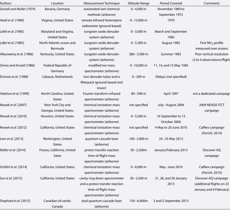
retrievals. Table 1 gives a list of representative NH3proﬁle measurements. The vertical evolution of NH3

emit-ted from the ground can be observed in the ﬁrst atmospheric layers with surface instruments [e.g., Erisman et al., 1988], but the majority of the measured proﬁles useful for satellite retrievals are acquired by airborne instruments. These cover a larger part of the tropospheric column, provide useful probing of the vertical distri-bution inside the column, and allow consistent validation of satellite quantities [e.g., Sun et al., 2015; Shephard et al., 2015; Van Damme et al., 2015a]. Nevertheless, the spatial and temporal coverage of such data sets is very heterogeneous, as the majority of observations are acquired during dedicated campaigns.

(6)

Table 1. NH3Vertical Measurements in the Literature

Authors Location Measurement Technique Altitude Range Period Covered Comments

Geordii and Muller [1974] Bavaria, Germany automated wet chemical 0–4,000 m November 1969 to methods (airborne) September 1972

Hoell et al. [1980] Virginia, United States remote infrared heterodyne 0–15,000 m 1979 radiometer (ground-based)

LeBel et al. [1985] Maryland and Virginia, tungsten oxide denuder 0–3,000 m March and September

United States system (airborne) 1983

LeBel et al. [1985] North Atlantic ocean and tungsten oxide denuder 0–5,300 m August 1982 First NH₃proﬁle

Bermuda system (airborne) measured over oceans

Alkezweeny et al. [1986] Kentucky, United States tungsten oxide denuder 380–3,580 m Summer 1983 Poor vertical resolution

system (airborne) (2 to 4 observations/ﬂight)

Ziereis and Arnold [1986] Federal Republic of modiﬁed ion mass 0–10,000 m 11, 14, and 15 May 1985 Germany spectrometer (airborne)

Erisman et al. [1988] Cabauw, Netherlands two denuder tubes and a 0–200 m 30days (not speciﬁed) ﬁlterpack (ground-based and

tower)

Yokelson et al. [1999] North Carolina, United Fourier transform infrared 84–598 m April 1997 not a dedicated campaign States spectrometer (airborne)

Nowak et al. [2007] New York City and chemical ionization mass not speciﬁed July–August 2004 2004 NEAQS-ITCT

Georgia, United States spectrometer (airborne) campaign

Nowak et al. [2010] Houston, United States chemical ionization mass 0–5,500 m 16 September to 13 spectrometer (airborne) October 2006

Nowak et al. [2012] California, United States chemical ionization mass not speciﬁed 4 May to 20 June 2010 CalNex campaign

spectrometer (airborne) [Parrish, 2014]

Leen et al. [2013] Washington, United quantum cascade laser 100–2,800 m 24–25 May 2012

States (airborne)

Müller et al. [2014] Fresno, California, United proton transfer reaction 30–2,500m January/February 2013 Discover-AQ

Sates time-of-ﬂight mass campaign

spectrometer (airborne)

Schiferl et al. [2014] California, United States chemical ionization mass 0–6,000 m May–June 2010 CalNex campaign

spectrometer (airborne) [Parrish, 2014]

Sun et al. [2015] California, United States cavity ring down spectrometer 30–2,500 m 21, 28, and 30 January Discover-AQ campaign and a proton transfer reaction 2013 (additional ﬂights on 23

time-of-ﬂight mass January and 6 February)

spectrometer (airborne)

Shephard et al. [2015] Canadian oil sands, dual quantum cascade laser 150–6,400m 3 and 5 September 2013

Canada (airborne)

As we will demonstrate, the proposed NN retrieval product can make optimal use of ancillary vertical profile data. However, given the limitations of in situ data, we will in first instance make use of vertical distributions from atmospheric models. While these have generally not been validated, a few local assessments have been performed when NH3vertical profile observations were available [e.g., Schiferl et al., 2014]. The spatial

resolu-tion of global models is also more representative for satellite instruments and allows a direct implementaresolu-tion of the NH₃vertical distributions in the retrieval processing chain.

2.2. A General Formula

From the previous section, it is clear that better accuracy in the retrieval will be achieved by considering realistic vertical profiles. Therefore, vertical profile information should be incorporated in the input param-eters in the NN. For this, it is necessary to parametrize the continuous vertical profile using a suitable analytical function. An analysis was made of the GEOS-Chem (www.geos-chem.org) v8.03.01 global chemical

(7)

Figure 2. Example of GEOS-Chem model (blue) and fitted (red) profiles (left) above a source area and (right) characteristic of transport withz₀,𝜎, and𝜌_maxindicated. The top right insets are histograms of𝜎derived from fitting of equation (2) to a representative set of GEOS-Chem profiles.

transport model (CTM) proﬁles for the year 2009. The GEOS-Chem oxidant-aerosol simulation includes H₂SO₄-HNO₃-NH₃aerosol thermodynamics coupled to an ozone-NO_x-hydrocarbon-aerosol chemical mech-anism [Park et al., 2004]. Partitioning of total ammonia and nitric acid between the gas and particle phases is calculated using the ISORROPIA II thermodynamic equilibrium model [Fountoukis and Nenes, 2007] as implemented in GEOS-Chem by Pye et al. [2009]. Among the functions that were tried, the following three-parameter Gaussian function was found to be able to approximate most GEOS-Chem proﬁles to good accuracy: 𝜌 = 𝜌maxe − ( z−z0 𝜎 )2 , (2)

with𝜌_maxthe maximum NH₃concentration (in ppb), z₀the peak height of the profile (in km), and𝜎 a mea-sure for the spread or thickness of the NH₃layer (in km). As an example, Figure 2 shows two vertical NH₃ profiles from GEOS-Chem (one representative for source (left), one for transport (right)), together with their Gaussian fit. We found that about 73% of the GEOS-Chem profiles could be fitted to a high accuracy with the proposed formula. The remaining profiles were found to have multiple maxima. The insets in Figure 2 are his-tograms of the𝜎 parameter of representative GEOS-Chem profiles with a NH₃total column larger than 5×1014

molecules.cm−2_{, separately for source (proﬁles peaking at the surface) and transported conditions. They show}

that most proﬁles have a𝜎 around 1 and virtually all modeled proﬁles a 𝜎 between 0 and 2.

3. The Neural Network

3.1. Training Set

The main idea of the proposed retrieval approach is to map the HRI to NH₃columns via a NN. As explained in section 1 a NN is built via training. Ideally, the training set should be as large, as accurate, and as extensive as possible, and input data in the training should be representative of the real input data. A description of the principles of operation of a supervised NN for atmospheric remote sensing can be found in Hadji-Lazaro et al. [1999], Turquety et al. [2004], and Blackwell and Chen [2009]. In this section, we explain how the NN training set was built.

Since a reference data set of IASI-NH3is not available, we built a synthetic training set using forward

simula-tions with the Atmosphit line-by-line radiative transfer model [Coheur et al., 2005]. To be representative for IASI observations, background atmospheric conditions were taken from 1year of thermodynamic atmospheric profiles provided by the meteorological Level 2 information from the operational IASI processor [August et al., 2012]. Most profiles (about 88%) were taken above land because of the larger variability encountered in the atmospheric conditions (e.g., thermal contrast, pressure profiles, and emissivity). NH3vertical profiles were

constructed following equation (2), where the three input parameters were varied randomly:𝜎 values were taken randomly between 0.25 and 2.5 km, and z0was set to 0 for 90% of the proﬁles (representative for

source proﬁles) and set randomly between 0 and 10km for the remaining 10% (representative for transported proﬁles).𝜌maxwas taken randomly between 0 and 20ppb. To account for background trace levels of NH3,

(8)

calculated as the mean of GEOS-Chem proﬁles with a NH₃column below 5 × 1014_molecules.cm−2_{. For the}

simulations, the vertical sampling of these NH₃proﬁles was set to 1 km with a ﬁner division of 0.2 km applied in a layer of 4 km around the peak height (z₀). About 250,000 IASI spectra were simulated both with and without NH₃(500,000 spectra in total).

We do not need the actual spectra as training data, but rather the derived HRI values. These were calcu-lated following equation (1) but with one important diﬀerence. From early tests, it was clear that simucalcu-lated spectra with a zero NH3column often had a rather large HRI value, probably related to inaccuracies in the

forward model. To make the training data set as accurate as possible, we simulated for each spectrum y a twin spectrum ywo, with a zero NH3column and calculated the HRI as

HRI = KT_S−1 y (y − ywo) √ KT_S−1 y K . (3)

The HRI calculated in this way is noise free (as mentioned in section 1, HRIs of spectra without observable NH3do have a mean HRI of 0 but a standard deviation of 1). Finally, note that in the calculation of the HRI

(equation (3)) we used angular dependent K,̄y, and S as in Bauduin et al. [2016] because of the dependence of the signal strength on the viewing angle. We refer to this paper also for a detailed explanation for the rational behind this.

3.2. The Setup, Training, and Evaluation

With the calculated HRI and the atmospheric parameters used for the construction of the associated spectra, we next trained the NN. We chose a supervised two-layer feedforward network: one hidden layer of 15 neurons with sigmoid transfer functions and one output layer of one linear neuron. The training was performed using the Levenberg-Marquardt backpropagation algorithm. For the training, the training set was divided into three distinct groups: (1) the training set strictly speaking, (2) a validation set, and (3) a test set. The selection of the training, validation, and test sets was performed randomly by considering a distribution of 85%-10%-5%. Eight diﬀerent parameters were selected as inputs for the NN. These are the surface temperature, the temperature, pressure, and humidity proﬁles, all four provided by the meteorological Level 2 information from the oper-ational IASI processor [August et al., 2012]; the𝜎 and z0parameters describing the shape of the NH3vertical

proﬁles; the surface emissivity (𝜖); and the viewing angle of the satellite. The temperature, pressure, and humidity proﬁles are described by 12, 11, and 7 levels, respectively. Surface emissivities over land were taken from the 2014 monthly mean spectral emissivity database provided by Zhou et al. [2011]. Over sea, emissivi-ties were taken from the Nalli et al. [2008] emissivity database. These spectral emissiviemissivi-ties were averaged over the range [800–1010; 1065–1200] cm−1_{. The 1010–1065 cm}−1_{region was excluded to avoid interferences}

from the𝜈3ozone band. The NN output parameter was set as the ratio of the NH3total column to the HRI. The

relationship between the input and the output parameters can be written as

NH3column = HRI × f (T, Tsurf, P, H2O, 𝜎, z0, 𝜖, angle). (4)

The rationale of using the ratio rather than the NH3total column itself is that the ratio has a smaller dynamic

scale, which allows for a much better training of the network. Also, working with the ratio ensures that the uncertainty on the HRI (mainly caused by instrumental noise) is translated in a linear way to the retrieved column. The sign of the ratio f will depend on the exact vertical proﬁle of NH3and the atmospheric

tempera-ture but will mostly follow the sign of the TC. Note that the ratio itself is totally independent of the HRI value (owing to the linear relationship between the HRI and the NH3column in the range of NH3column values

usually encountered), and that noise on the HRI can result in negative NH3columns. This has a number of

beneﬁts which will be discussed further on.

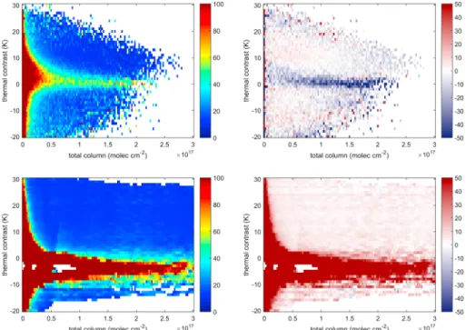
To assess the performance of the training, we have calculated for the whole training set the mean relative error and relative bias of the retrieved columns (̂y) over the actual columns y per bin of 1 K of TC and 2.5×1015

molecules.cm−2_{of NH} 3total column: Error = 1 n n ∑ k=1 || ||̂yky− yk k || ||× 100, (5)

(9)

Figure 3. Evaluation of the training of the neural network. The color bar represents (left column) the mean error (%) and (right column) bias (%) between the real state and the output from (top row) the NN-based and (bottom row) the LUT-based HRI method used in Van Damme et al. [2014a].

Bias = 1 n n ∑ k=1 ̂yk− yk yk × 100. (6)

To make the assessment more representative of real IASI measurements, we have added normally distributed noise on the HRI. The results are shown in Figure 3 as a function of TC and NH3column. To compare, the mean

error and bias calculated from the LUT-based HRI method are given as well (here we used the forward sim-ulations used to build the LUT). The TC (K), which drives the sensitivity of the IR measurements to boundary layer concentrations, is defined here as the difference between the surface temperature and the temperature at 1.5 km of altitude. The comparison between the two methods shows a clear improvement of the NN com-pared to the LUT, both in the mean and the bias, especially for low TCs. As expected, largest errors (>100%) are found for low TCs (low sensitivity) since a large fraction of NH3vertical profiles peak at the surface (z0= 0)

and rapidly decrease with altitude. Relative errors are also large for low NH3total columns (but in this case

absolute errors can still be small).

For the NN-based method, the mean error rapidly decreases with increasing TC and total column and becomes lower than 30% (40%) for TC above (below) +10 K (−10 K) and total column higher than about 5 × 1016

molecules.cm−2_{. The corresponding mean bias is generally below 10% except at low TC (between 0 and 5 K)}

for high NH3columns (>1×1017molecules.cm−2) where an underestimation of about 40% is observed. For the

LUT-based method in contrast, a large mean overestimation (>50%) is observed at low NH3columns or low

TC up to high total columns (>3 × 1017_{) but associated with large mean uncertainties (}_{>100%). This}

overesti-mation is due to the instrumental error on the HRI (represented here by the random noise added on the HRI) which results in a nonzero HRI, even in the absence of NH₃. In the LUT-based HRI method, these nonzero HRIs are converted into positive NH₃total columns introducing therefore a systematic positive bias in the mean. In contrast, in the NN-based method this bias is lower owing to the parametrization of the NN which allows negative value of NH₃columns for low (positive or negative) values of HRI, resulting in a mean bias close to 0.

3.3. Retrieval, Uncertainty Estimate, and Example

For the actual retrieval we first filtered out observations with a cloud fraction inside the IASI field of view above 25%, since our training data did not include clouds. Then for the remaining observations the different input parameters of the NN were gathered. Atmospheric profiles (water vapor, pressure, and temperature) were

(10)

taken from the IASI meteorological L2. Surface emissivities were taken as the mean of the spectral emissivity in the range [800–1010; 1065–1200] cm−1_{from the 2014 monthly mean database provided by Zhou et al. [2011]}

(for land measurements) and from the Nalli et al. [2008] database for sea measurements. HRIs were calculated following equation (1) (with again angular dependent K,̄y, and S). In first instance, and to ease comparison with the LUT product, we used fixed values for the𝜎 and z0input parameters by fitting the single NH3profiles

used for land and sea in the LUT-based HRI method [Van Damme et al., 2014a]. We found z0= 0;𝜎 = 1.07 km

and z0= 1.4; 𝜎 = 1.28 km for land and sea proﬁles respectively. These are used as default values for 𝜎 and z0,

unless speciﬁcally otherwise stated.

After application of the network, a ﬁlter is applied to remove unphysical retrievals associated with errors in the input parameters. Retrievals are removed when (1) negative columns are associated with a HRI above 1.5 in absolute value and (2) the ratio of NH3column to the HRI is higher than 3 × 1016. The ﬁrst criterion guarantees

that negative columns are only possible for NH3retrievals within the IASI noise. The second criterion removes

retrievals where a large HRI is observed corresponding to an almost zero TC (thus likely caused by errors in the TC or NH₃proﬁle). This procedure removes between 5% and 10% of the data, mostly with evening overpasses. To each retrieved NH3total column an associated uncertainty can be estimated by propagating the

uncer-tainties of the diﬀerent parameters of the NN following

sNH3= √( 𝜕NH3 𝜕HRI )2 s2 HRI+ ( 𝜕NH3 𝜕T )2 s2 T+ ( 𝜕NH3 𝜕Tskin )2 s2 Tskin+ ( 𝜕NH3 𝜕H2O )2 s2 H2O+ ( 𝜕NH3 𝜕𝜎 )2 s2 𝜎. (7)

Here sNH3is the absolute uncertainty on the NH3column. sTand sH2Oare the uncertainty on the temperature

profile and the water vapor profile, respectively, which are set at 1 K for each level of the temperature profile and at 10% for the levels of water vapor profile, based on early validation of the IASI Level 2 meteorological fields [Pougatchev et al., 2009]. s_Tskinis the uncertainty on the surface temperature and is conservatively set to 1 K. s_HRI and s_𝜎 are the standard deviation of the HRI and𝜎 and are set to 1 (per definition) and 0.5 (see histogram of𝜎 in Figure 2), respectively. s_𝜎is used to evaluate the uncertainty associated with the retrieval sensitivity to the vertical distribution of NH3. Note that cloud coverage, by affecting the value of the calculated

HRI, also inﬂuences the retrieval. An analysis over Europe in the summer showed that the impact of clouds on the HRI is almost linear up to high values with a slope close to −1 (a 25% cloud coverage causes on average a roughly equal decrease of the HRI). Although the 25% threshold is arbitrary, it is a good compromise between keeping the number of measurements high and the impact of clouds low. This is important to keep in mind for the utilization of the product.

An example of retrieved NH3total columns (molecules.cm−2) on 2 June 2013 for the morning (top) and the

evening (bottom) overpasses of IASI is given in Figure 4. Light gray points correspond to cloudy pixels. The cor-responding distributions of the uncertainty are shown in the inset. Large columns are, for example, observed above the usual agricultural hot spots. The large columns observed over the Paciﬁc Ocean near the west coast of Mexico correspond to transported plumes emitted by biomass burning in this region. Diﬀerences observed between morning and evening overpasses of IASI could be due to diurnal variations of NH3but have not been

further investigated.

An appealing feature is that the retrieved NH₃total columns (moleculesm−2_{) for areas far away from source}

regions (such as over most of the oceans) are close to 0. As explained, this is due to the fact that retrieval noise is translated in a linear way into the retrieved columns. Therefore, and because of the deﬁnition of HRI, the retrieved values over remote areas will follow a Gaussian distribution around zero, guaranteeing an average close to 0. However, over certain regions (e.g., for this day, over Bolivia and Peru), negative NH3columns are

predominant, especially for the evening overpass. This bias is either caused by a bias in the HRI (e.g., due to sur-face effects) or by incompatible meteorological L2 data (for instance, relative high HRI values corresponding to areas with a negative TC). Most of these observations are already removed by the filter mentioned above, but as it is quite conservative it does not remove all the anomalies. An analysis of data from different years (2008–2015) revealed that the anomalous negative values occur less frequently with newer L2 data, indicating improvements in the IASI L2 products. The analysis of the uncertainty distribution reveals uncertainties gener-ally below 30% (50%) over the identified source areas for the morning (evening) overpass time measurements. For regions with low NH3columns in contrast, the uncertainty is typically larger than 150%.

(11)

Figure 4. NH₃total column distributions (molecules.cm−2_{) for (top) the morning and (bottom) the evening overpasses} of IASI on Metop-A for 2 June 2013. Associated uncertainty distributions (%) are shown as well (bottom left inset).

3.4. Uncertainty Characterization

An example of uncertainties and their partitioning in the diﬀerent uncertainty contributions is shown in Figure 5 for measurements selected on 15 June 2013 (morning overpass time). Four cases characterized by dif-ferent sensitivity to the measurement (TC) and NH3column were considered: (1) high NH3column (∼ 9 × 1016

molecules.cm−2_{) and high TC (∼15 K, high sensitivity); (2) high NH}

3column (∼9 × 1016molecules.cm−2) and

low TC (∼3 K, low sensitivity); (3) low NH3column (∼ 4.5 × 1015molecules.cm−2) and high TC (∼14 K); and (4)

low column (∼ 4.5 × 1015_molecules.cm−2_{) and low TC (∼2 K).}

The lowest uncertainties are around 25% when high columns and high TC coincide. When either of these decrease, the uncertainty progressively increases. For these cases, uncertainties are found up to 85–148%. When both the TC and column are low, all sensitivity to NH3is lost. In case of high TC and high NH3columns

(high HRI), the major relative contribution to the total uncertainty comes from the thickness of the NH3layer

(𝜎) (36%) followed by the surface temperature (24%) and the temperature proﬁle (16%). The relative contri-bution of the HRI is low (11%) since HRI is large in absolute value (because of the large TC and large column). For low TC and high NH₃column, the sensitivity of the retrieved NH₃total column to small variations of the TC and HRI is larger. This results in a higher relative contribution of the HRI (17%), surface temperature (25%), and temperature proﬁle (19%), while the relative contribution of the𝜎 parameter is reduced (22%).

(12)

Figure 5. Example of error distributions of the NH₃retrieved columns for diﬀerent situations characterized by diﬀerent sensitivity to the measurements and NH₃total column. From left to right: (1) high NH₃column (∼ 9 × 1016

molecules.cm−2_{) and high TC (}_∼_{15 K), (2) high column (}_{∼ 9 × 10}16_molecules.cm−2_{) and low TC (}_∼_{3 K), (3) low column} (∼ 4.5 × 1015molecules.cm−2_{) and high TC (}_∼_{14 K), and (4) low column (}_{∼ 4}_{.5 × 10}15_molecules.cm−2_{) and low TC (}_∼_{2 K).} The total relative error for each case is given as well.

For high TC and low NH3column in contrast, the major contribution to the total uncertainty is on the HRI,

reaching 67%, because in this case the uncertainty on the HRI (one by deﬁnition) can be comparable or even larger than the value of the HRI. In this case this uncertainty dominates all other contributions. Finally, for low TC and low NH₃column (low HRI), the relative uncertainty on the retrieved column is very large (270%), and compared to the previous case, also uncertainties on the other parameters become more important. It is clear that such measurements are of limited usefulness.

3.5. NN Versus LUT Retrievals

In this section we compare retrievals of the LUT-based and the NN-based HRI method. For this, all measure-ments for the year 2013 with a relative uncertainty below 100% were selected. A scatterplot between the two retrievals over land is shown in Figure 6. Three main patterns stand out (numbered (1)–(3) in the ﬁgure): 1. For measurements where both algorithms give a relative uncertainty below 25%, the retrieved NH3

columns from the NN-based and the LUT-based method are in excellent agreement (543,847 mea-surements in total with a correlation coeﬃcient of 0.91 and linear regression (Pearson’s major axis) of NN = LUT × 0.85 − 0.17 × 1016_{). These correspond to measurements associated with high TC (}_{>15 K) and a}

high HRI (>10). A similar analysis was made for retrievals over oceans only (not shown here). While the cor-relation coeﬃcient for the measurements over sea is relatively good (0.87), the linear regression indicates larger diﬀerences than for land (NN = LUT × 1.19 − 0.72 × 1016_{; 1574 measurements in total).}

2. The measurements in this group are associated with a relative uncertainty mainly comprising between 25% and 75% and a high HRI (>10) but a fairly low positive TC (5–10K). The retrieved columns derived from the NN are consistently larger than the columns retrieved from the LUT (more than a factor of 2). A possible reason for these differences is that the LUT was derived from averages of forward simulations using many different background atmospheres, which could be affected by outliers.

3. These measurements have a low HRI (−3<HRI<3) and TC (−5 <TC<5 K). Here the sensitivity to atmospheric NH3is low. The columns retrieved from the NN are generally much smaller than for those retrieved from the

LUT. The existing bias in the LUT is the largest for these retrievals, and the reduction of this bias in the NN can be seen clearly (with an average close to 0). Over sea, the majority of the observations belongs to this category, and an even larger scatter is observed between the LUT and NN.

(13)

Figure 6. NH₃total columns (molecules.cm−2_{) retrieved from the NN-based method (y axis) versus those retrieved from} the LUT-based method (x axis) over the entire year 2013 (morning and evening overpasses) over land. The colors refer to the uncertainty (%) associated with the total columns retrieved from the NN-based method. Numbering (1)–(3) corresponds to the main patterns standing out. These correspond to measurements associated with (1) a high TC and a high HRI, (2) a high HRI and a low positive TC, and (3) a low HRI and TC.

4. Impact of the NH

₃

Vertical Proﬁles

One of the advantages of the NN-based method is that it allows using variable NH3proﬁles. As shown in

section 2.1, the vertical distribution can have a large impact on the retrieved total column. To give an idea of the potential impact on a global scale, we have retrieved NH3columns assuming that most NH3is located in

the planetary boundary layer (PBL) by setting𝜎 equal to the PBL height derived from the ERA-interim reanal-ysis [Dee et al., 2011]. Note that for PBL heights lower than 250m, the𝜎 value has been set to 250m since the NN has not been trained for lower values. Figure 7 shows the relative diﬀerence (%) between the retrieval using the ﬁxed𝜎 derived from the LUT (=1.07 km for land) and the retrieval using the PBL height for 2 June 2013 (morning orbits, land only). Corresponding PBL height (km) and TC distributions (now taken at 1 km) are provided as well (bottom left and bottom right insets, respectively). Highly variable PBL heights are observed

Figure 7. Relative diﬀerences (%) between NH₃total columns (molecules.cm−2_{) retrieved over land for 2 June 2013 (morning orbits) using a ﬁxed}_𝜎_{(=1.07 km for} land) and using the PBL height from the ERA-interim reanalysis as𝜎. The bottom left and bottom right insets show the corresponding PBL height (km) and TC (K,T_surf− T_1km) distributions, respectively.

(14)

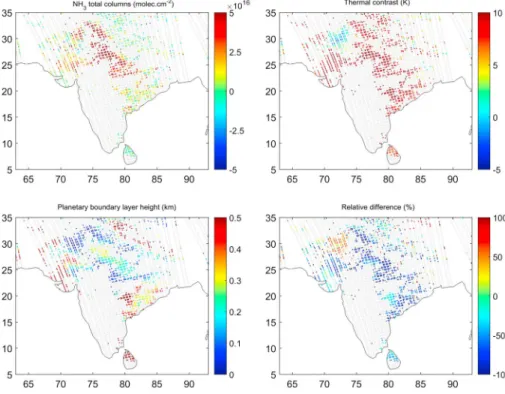
Figure 8. (top left) Nighttime IASI-NH₃total column (molecules.cm−2_{) distribution for 2 June 2013 over India retrieved} by considering a fixed𝜎, (top right) associated TC (K,T_surf− T_1km) and (bottom left) PBL height (km), and (bottom right) relative differences (%) between NH₃total columns (molecules.cm−2_{) distributions retrieved using a fixed}_𝜎_{(=1.07 km} for land) and using the PBL height from the ERA-interim reanalysis as𝜎.

globally ranging from above 0 km to more than 2.5 km. The largest diﬀerences in the retrieved NH₃columns are between 60% and 100% (e.g., in the Southern Hemisphere and at high latitudes). Since the PBL height is spa-tially highly variable, no clear geographical patterns can be discerned. In case of positive TC (which is almost always the case here), the retrieved NH3columns will generally be lower for NH3proﬁles with a thicker layer

because of the better sensitivity to NH3at higher altitude—and conversely. This is consistent with Figure 1.

The impact of the NH3vertical proﬁle on the retrieved column for a nighttime distribution is shown in Figure 8

(bottom right). As the sensitivity is generally lower for nighttime measurements (due to a general lower TC), we focus only on a source region (South Asia) and land proﬁles. The nighttime NH3total column distribution

retrieved for a ﬁxed𝜎 (Figure 8, top left), and corresponding TC (Figure 8, top right) and PBL height (Figure 8, bottom left) distributions are also shown. At night, the PBL height is generally much lower than during the day [Jacob, 1999]. For the region shown, the PBL is mostly below 500m. The TC distribution is mostly positive, except over Pakistan where slightly negative values are observed. As for the daytime distribution, for a given signal in the IASI spectra, lower𝜎 values combined with positive TCs result in higher retrieved NH3columns

with relative difference up to 100%. In contrast, for the area showing slightly negative values of TC, the retrieved columns are about 20–30% lower than the retrieved columns using a fixed𝜎. The magnitude of these differences is in line with what was shown in section 2.1.

5. Global Annual Mean and the Importance of the Averaging Procedure

For some applications, it is useful to consider monthly or yearly average distributions. However, as discussed in Van Damme et al. [2014a], averaging is not straightforward because of large variability of the NH3

measure-ment sensitivity. It can for instance happen that the arithmetic mean of a group of observations is dominated by a single anomalous high measurement value (corresponding to a measurement with low sensitivity and high uncertainty). Averages from the LUT retrieval approach suﬀered from such measurements. For this reason Van Damme et al. [2014a] made use of weighted averages, where the weight was taken inversely proportional to the square of the estimated uncertainty of the measurement (in relative or absolute terms). Therefore, measurements thought to have a high accuracy carry a larger weight in the average. Another approach is to

(15)

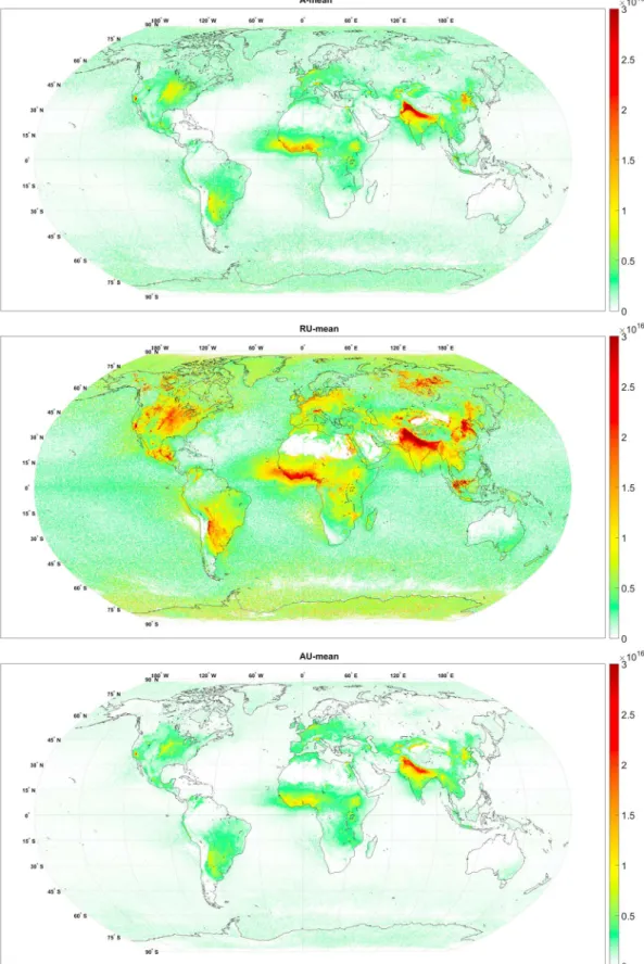
Figure 9. NH₃total columns (molecules.cm−2_{) distributions from IASI measurements for the year 2013, in a 0.25}∘_by

0.25∘grid for the morning overpasses. NH₃distributions are a mean of all measurements within a cell following (top) an arithmetic mean (A-mean), (middle) a weighted mean by the relative uncertainty (RU-mean), and (bottom) a weighted mean by the absolute uncertainty (AU-mean).

(16)

remove those measurements for which the uncertainty exceeds a certain threshold value (this is equivalent to using 0/1 weights). The disadvantage of weighting approaches is that they bias the average: for instance, 0/1 weighting or weighting with the relative error will favor the largest columns with a low uncertainty; weighting with an absolute error will favor the lowest columns. Figure 9 illustrates three diﬀerent averaging procedures: arithmetic mean (A-mean, top), weighted mean by the relative uncertainty (RU-mean, middle), and the abso-lute uncertainty (AU-mean, bottom). In all three cases we used all retrievals of the morning overpass of the year 2013 but removed grid cells with less than 15 observations. For more details on the weighted averaging procedure, we refer to Van Damme et al. [2014a].

A main feature to notice in Figure 9 is that, despite the diﬀerent averaging procedures, the mean NH₃total columns are of the same order of magnitude. This indicates that anomalous high or low measurements are not as important for the NN as for the LUT. Analyzing the daytime distribution reveals the same main NH3hot spots

that were identiﬁed by Van Damme et al. [2014a], mainly related to ﬁre and agriculture. For agricultural sources, we observe large NH3columns especially above the Indo-Gangetic Plain, the Fergana Valley in Central Asia, the

North China Plain in Asia, the US Midwest region and San Joaquin Valley, the Po valley, and the Netherlands in Europe. NH₃hot spots associated with biomass burning are found, for example, above central Africa, Eastern Russia, Thailand, and Indonesia. For a more complete analysis of the NH₃sources and hot spots, we refer to Van Damme et al. [2014a]. However, the comparison between the different averaging methods highlights important differences in the regions with large NH3columns. In particular, a large impact of fire plumes is

revealed in the RU-mean due to the better sensitivity of IASI for NH3at higher altitude [Van Damme et al.,

2014a, 2014b]. High NH3columns related to ﬁres emissions are, for example, observed above Canada, Eastern

Russia, and Indonesia. Moreover, many localized hot spots show up, especially above the US and Western Russia. In contrast, in the AU-mean only the permanent hot spots of NH₃total columns appear (these are principally related to agriculture). Hot spots associated with biomass burning are generally not visible, due to the more important weight given to the low columns (with a lower absolute uncertainty). Mean NH3columns

are therefore also lower than in the RU-mean. The A-mean is relatively close to the AU-mean but reveals slightly better the biomass burning hot spots (e.g., Eastern Russia). We conclude that with the proposed NN product, the expected differences between the different averaging procedures are still present but less pronounced. The choice of averaging procedure will principally be determined by the specific application.

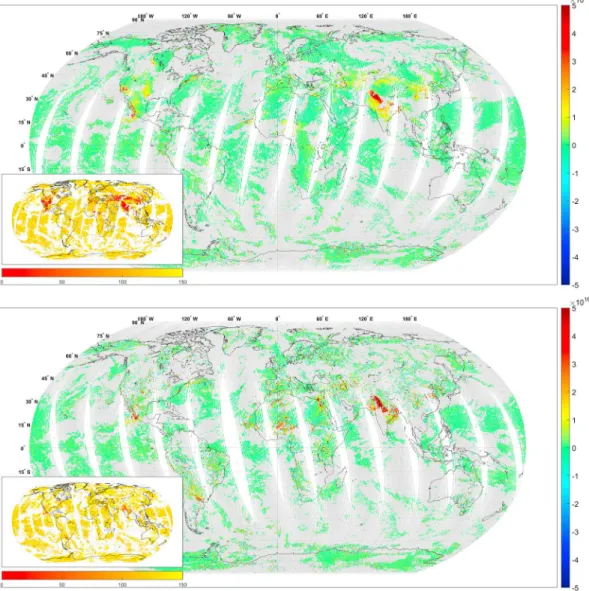
6. Comparison With GEOS-Chem

In this section we compare the mean NH₃global distributions to those simulated with the GEOS-Chem CTM. The GEOS-Chem v8.03.01 model provides NH3total columns on a daily basis with a horizontal resolution of

2∘ × 2.5∘. One of the advantages of the new product is that it can use profile information from other sources. To compare optimally with GEOS-Chem, it therefore makes sense to use collocated vertical profile shape information in the retrieval.𝜎 and z₀values were obtained for each IASI observation by fitting the Gaussian profile (equation (2)) to the corresponding GEOS-Chem grid cell sampled at the same time as the IASI overpass. Note that we only considered IASI observations and corresponding GEOS-Chem modeled for which the GEOS-Chem profile could be fitted to a high accuracy (∼73% of all profiles). The global NH3mean

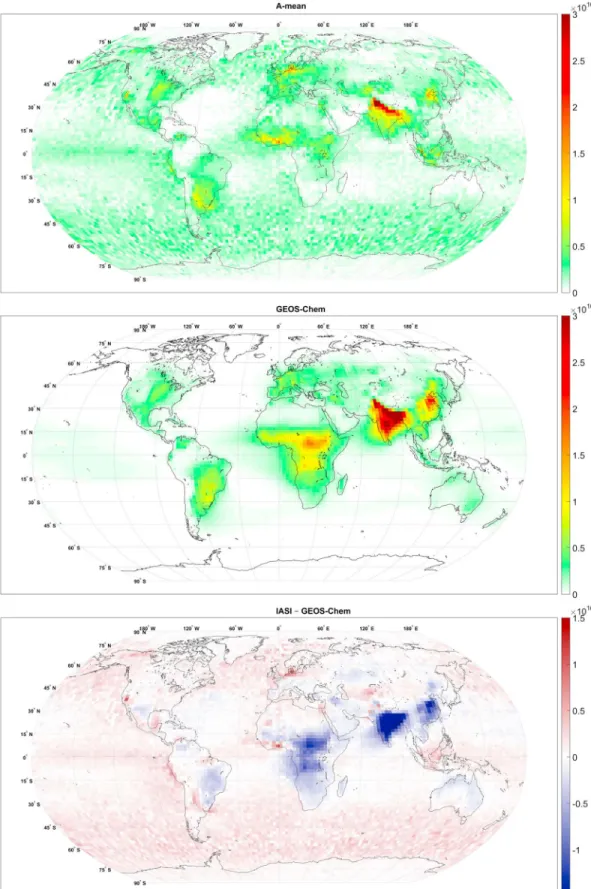
distribu-tions derived from IASI measurements and given by the GEOS-Chem simuladistribu-tions for the year 2009 are shown in Figure 10 (top and middle, respectively). The absolute diﬀerences between the two distributions are also shown (Figure 10, bottom).

The same main source areas are found both in the satellite and modeled distributions. Also, transport pat-terns over oceans are in very good agreement (off the west coast of Africa, Indian Ocean, Mediterranean Sea, and off the east of South America). However, some source areas appear to be more concentrated in the IASI distributions. This is in particular the case for India for which the highest IASI columns are confined to the Indo-Gangetic plain, while GEOS-Chem simulates very high columns over most of India and Pakistan. On a quantitative level, IASI and GEOS-Chem are consistent on a yearly basis over most of the Northern Hemisphere within ±3 × 1015_molecules.cm−2_{. However, an overestimation of GEOS-Chem simulations over IASI}

measure-ments of about 1–1.5 × 1016_molecules.cm−2_{is found for India and the North China plain. Overestimations of}

about 0.7–1×1016_molecules.cm−2_{are found as well over Central Africa. IASI columns are larger only for certain}

hot spots (the San Joaquin Valley, the Netherlands, and West Africa). Considering the generally strong positive thermal contrast prevailing during daytime, these observed diﬀerences between IASI and GEOS-Chem distri-butions (about 50–70% over the source areas) appear to be too high to be only explained by the reported bias on the training data set (for TC>5–10K) (Figure 3).

(17)

Figure 10. (top) NH3total columns (molecules.cm−2) distributions from IASI measurements for the year 2009, in a 2.5∘ by 2∘grid for the morning overpasses.𝜎values were selected by fitting the corresponding GEOS-Chem NH3vertical profiles. (middle) NH₃total columns (molecules.cm−2_{) distributions from the GEOS-Chem CTM. (bottom) Differences} between NH₃total columns (molecules.cm−2_{) distributions measured by IASI and simulated by GEOS-Chem.}

(18)

7. Conclusion

In this paper we have introduced a new neural network (NN)-based NH₃retrieval algorithm. It combines most advantages of full ﬁtting approaches with HRI based approaches. To recapitulate, from the latter it inherits the following:

Computational Eﬃciency. The only parameter retained from the measurement is the HRI value. Calculating

these is straightforward and computational time is negligible. Calculating the neural network function F is equally straightforward.

Full Spectral Range. The HRI takes into account the spectral range 800–1200 cm−1_{, which contains all the}

important NH₃lines in the infrared, and thereby takes full advantage of the thermal infrared.

Low Dependency on the Forward Model. The forward model is only of secondary importance for the

calcula-tion of the Jacobians in the HRI and also for the HRI calculated from the NN training data. Because we use an angular dependent gain matrix, the NN-based approach removes the residual angular dependency previously reported in Van Damme et al. [2014a].

No A Priori Information. No a priori information on the column is used. This means that all the information

from the ﬁnal measurement comes from the spectral measurement (but potentially with very large associated uncertainty estimates). So in contrast to optimal estimation approaches, no averaging kernel needs to be applied when carrying out comparison with other measurements/models. A priori information on the vertical proﬁle shape is used though.

The main advantages of the NN over the LUT-based HRI method are the following:

Full Atmospheric State. Because the number of input parameters is not limited in the NN, the full temperature,

humidity, and pressure proﬁles can be taken into account. This property is shared with the spectral ﬁtting approaches.

Full Uncertainty Analysis. By perturbing the input parameters a full uncertainty characterization can be made

of how the uncertainty of each of the input parameters propagates to the ﬁnal result. This analysis can be carried out on a per-pixel basis.

Reduced Bias. Rather than mapping the input parameters directly to a NH3column, the output of the NN is

a scaling factor, which after multiplication with the HRI gives the column. In this way, the instrumental error on the HRI is translated in a linear way in an error on the column, and negative columns become possible. At the same time, this implies that the algorithm itself is not biased high as was the case with the LUT-based conversion (this is assuming that the HRI values themselves are not biased). At least for making averaged distributions, this decreased bias helps to reduce the importance of the precise averaging procedure that is used.

Flexible NH3Profiles. All the retrieval approaches which have been used so far assume a fixed or an a priori NH3vertical profile. While infrared sounders have limited or no sensitivity to the vertical profile of NH3, the

assumptions on the profile can affect the retrieved column greatly. It is clear, even from the limited amount of in situ measurements, that the vertical profiles of NH3exhibit a huge variability. To deal with this, we have

included two input parameters in the NN describing the proﬁle, namely, the peak height and the thickness of the NH3layer. This allows to estimate robustly the uncertainty in the retrieved column due to the uncertainty

in the assumed proﬁle but also allows the following:

1. Study of wildfire emissions. Using a fixed NH₃profile can yield large errors on the retrieved column espe-cially when studying wildfire plumes which can have a peak altitude several kilometers above the surface. Coupling bottom-up [Sofiev et al., 2012] or top-down [Val Martin et al., 2010] height estimates could therefore greatly improve the accuracy of satellite retrievals of NH3in wildfire plumes.

2. Model exploitation possibilities. The flexibility in NH₃ vertical profiles can in the future be exploited to improve atmospheric chemistry-transport models. In evaluating a chemical transport model, retrievals can be carried out using the modeled NH3profile for a more consistent comparison. Improvements in, e.g.,

dispersion and lifetime of the model could then be evaluated from the retrievals carried out with updated proﬁles.

3. In situ measurements. In situ measurements of NH3proﬁles or boundary layer heights can be directly utilized

to improve satellite retrievals and/or validation exercises, as suggested in Van Damme et al. [2015a]. Here we have demonstrated that these can greatly alter the retrieved columns on a global scale.

(19)

North Carolina, J. Air Waste Manage. Assoc., 54(5), 623–633, doi:10.1080/10473289.2004.10470933.

Bauduin, S., L. Clarisse, J. Hadji-Lazaro, N. Theys, C. Clerbaux, and P.-F. Coheur (2016), Retrieval of near-surface sulfur dioxide (SO2)

concentrations at a global scale using IASI satellite observations, Atmos. Meas. Tech., 9(2), 721–740, doi:10.5194/amt-9-721-2016. Beer, R., M. W. Shephard, S. S. Kulawik, S. A. Clough, A. Eldering, K. W. Bowman, S. P. Sander, B. M. Fisher, V. H. Payne, M. Luo,

G. B. Osterman, and J. R. Worden (2008), First satellite observations of lower tropospheric ammonia and methanol, Geophys. Res. Lett., 35, L09801, doi:10.1029/2008GL033642.

Behera, S. N., M. Sharma, V. P. Aneja, and R. Balasubramanian (2013), Ammonia in the atmosphere: A review on emission sources, atmospheric chemistry and deposition on terrestrial bodies, Environ. Sci. Pollut. Res. Int., 20(11), 8092–8131,

doi:10.1007/s11356-013-2051-9.

Blackwell, J., and F. Chen (2009), Neural Networks in Atmospheric Remote Sensing, Artech House Massachusetts Institute of Technology, Boston.

Clarisse, L., C. Clerbaux, F. Dentener, D. Hurtmans, and P.-F. Coheur (2009), Global ammonia distribution derived from infrared satellite observations, Nat. Geosci., 2(7), 479–483, doi:10.1038/ngeo551.

Clarisse, L., M. Shephard, F. Dentener, D. Hurtmans, K. Cady-Pereira, F. Karagulian, M. Van Damme, C. Clerbaux, and P.-F. Coheur (2010), Satellite monitoring of ammonia: A case study of the San Joaquin Valley, J. Geophys. Res., 115, D13302, doi:10.1029/2009JD013291. Clarisse, L., P.-F. Coheur, F. Prata, J. Hadji-Lazaro, D. Hurtmans, and C. Clerbaux (2013), A uniﬁed approach to infrared aerosol remote sensing

and type speciﬁcation, Atmos. Chem. Phys., 13(4), 2195–2221, doi:10.5194/acp-13-2195-2013.

Clerbaux, C., et al. (2009), Monitoring of atmospheric composition using the thermal infrared IASI/MetOp sounder, Atmos. Chem. Phys., 9, 6041–6054, doi:10.5194/acp-9-6041-2009.

Coheur, P.-F., B. Barret, S. Turquety, D. Hurtmans, J. Hadji-Lazaro, and C. Clerbaux (2005), Retrieval and characterization of ozone vertical proﬁles from a thermal infrared nadir sounder, J. Geophys. Res., 110, D24303, doi:10.1029/2005JD005845.

Coheur, P.-F., L. Clarisse, S. Turquety, D. Hurtmans, and C. Clerbaux (2009), IASI measurements of reactive trace species in biomass burning plumes, Atmos. Chem. Phys., 9, 5655–5667, doi:10.5194/acp-9-5655-2009.

Dee, D. P., et al. (2011), The ERA-Interim reanalysis: Conﬁguration and performance of the data assimilation system, Q. J. R. Meteorol. Soc., 137(656), 553–597, doi:10.1002/qj.828.

Erisman, J.-W., A. W. Vermetten, W. A. Asman, A. Waijers-Ijpelaan, and J. Slanina (1988), Vertical distribution of gases and aerosols: The behaviour of ammonia and related components in the lower atmosphere, Atmos. Environ., 22(6), 1153–1160, doi:10.1016/0004-6981(88)90345-9.

Flechard, C. R., E. Nemitz, R. I. Smith, D. Fowler, A. T. Vermeulen, A. Bleeker, J. W. Erisman, D. Simpson, L. Zhang, Y. S. Tang, and M. A. Sutton (2011), Dry deposition of reactive nitrogen to European ecosystems: A comparison of inferential models across the NitroEurope network, Atmos. Chem. Phys., 11(6), 2703–2728, doi:10.5194/acp-11-2703-2011.

Fortems-Cheiney, A., et al. (2016), Unaccounted variability in NH₃agricultural sources detected by IASI contributing to European spring haze episode, Geophys. Res. Lett., 43, doi:10.1002/2016GL069361, in press.

Fountoukis, C., and A. Nenes (2007), ISORROPIA II: A computationally eﬃcient thermodynamic equilibrium model for K+-Ca2+-Mg2+-NH+₄-Na+-SO2−₄ -NO3−-Cl−-H₂O aerosols, Atmos. Chem. Phys., 7(17), 4639–4659.

Geordii, H. W., and W. J. Muller (1974), On the distribution of ammonia in the middle and lower troposphere, Tellus, 26(1–2), 180–184, doi:10.1111/j.2153-3490.1974.tb01965.x.

Hadji-Lazaro, J., C. Clerbaux, and S. Thiria (1999), An inversion algorithm using neural networks to retrieve atmospheric CO total columns from high-resolution nadir radiances, J. Geophys. Res., 104(D19), 23,841–23,854.

Heald, C. L., J. L. Collett Jr., T. Lee, K. B. Benedict, F. M. Schwandner, Y. Li, L. Clarisse, D. R. Hurtmans, M. Van Damme, C. Clerbaux, P.-F. Coheur, S. Philip, R. V. Martin, and H. O. T. Pye (2012), Atmospheric ammonia and particulate inorganic nitrogen over the United States, Atmos. Chem. Phys., 12(21), 10,295–10,312, doi:10.5194/acp-12-10295-2012.

Hilton, F., et al. (2011), Hyperspectral Earth observation from IASI: Five years of accomplishments, Bull. Am. Meteorol. Soc., 93(3), 347–370, doi:10.1175/BAMS-D-11-00027.1.

Hoell, J. M., C. N. Harward, and B. S. Williams (1980), Remote infrared heterodyne radiometer measurements of atmospheric ammonia proﬁles, Geophys. Res. Lett., 7(5), 313–316, doi:10.1029/GL007i005p00313.

Jacob, D. J. (1999), Introduction to Atmospheric Chemistry, Princeton Univ. Press, Princeton, N. J.

LeBel, P. J., J. M. Hoell, J. S. Levine, and S. A. Vay (1985), Aircraft measurements of ammonia and nitric acid in the lower troposphere, Geophys. Res. Lett., 12(6), 401–404, doi:10.1029/GL012i006p00401.

Leen, J. B., X.-Y. Yu, M. Gupta, D. S. Baer, J. M. Hubbe, C. D. Kluzek, J. M. Tomlinson, and M. R. Hubbell (2013), Fast in situ airborne measure-ment of ammonia using a mid-infrared oﬀ-axis ICOS spectrometer, Environ. Sci. Technol., 47(18), 10,446–10,453, doi:10.1021/es401134u. Luo, M., M. W. Shephard, K. E. Cady-Pereira, D. K. Henze, L. Zhu, J. O. Bash, R. W. Pinder, S. L. Capps, J. T. Walker, and M. R. Jones (2015),

Satellite observations of tropospheric ammonia and carbon monoxide: Global distributions, regional correlations and comparisons to model simulations, Atmos. Environ., 106, 262–277, doi:10.1016/j.atmosenv.2015.02.007.

Müller, M., et al. (2014), A compact PTR-ToF-MS instrument for airborne measurements of volatile organic compounds at high spatiotemporal resolution, Atmos. Meas. Tech., 7(11), 3763–3772, doi:10.5194/amt-7-3763-2014.

Nalli, N., P. Minnett, and P. van Delst (2008), Emissivity and reﬂection model for calculating unpolarized isotropic water surface-leaving radiance in the infrared. I: Theoretical development and calculations, Appl. Opt., 47(21), 3701–3721, doi:10.1364/AO.47.004649. part of the EUMETSAT Polar System.

The IASI L1 data are received through the EUMETCast near-real-time data distribution service. The research in Belgium was funded by the F.R.S.-FNRS and the Belgian State Federal Office for Scientific, Technical and Cultural Affairs (Prodex arrangement IASI.FLOW). S. Whitburn is grateful for his PhD grant (Boursier FRIA) to the “Fonds pour la Formation à la Recherche dans l’Industrie et dans l’Agriculture” of Belgium. L. Clarisse is Research Associate (Chercheur Qualifié) with the Belgian F.R.S.-FNRS. S. Bauduin is Research Fellow with F.R.S-FNRS. C. Clerbaux is grateful to CNES for scientific collaboration and financial support. C. L. Heald acknowledges support from NOAA (NA12OAR4310064). M.A. Zondlo acknowledges support from NASA (NNX14AT36G, NNX14AT32) and the Satellite Application Facility on Ozone and Atmospheric Chemistry Monitoring (O3MSAF) of European Organization for the Exploitation of Meteorological Satellites (EUMETSAT).