Noctilucent clouds and the mesospheric water vapour: the past decade
Texte intégral
Figure

![Table 3. Summer means of NLC backscatter coefficients β and β n at the layer peaks and NLC occurrence probabilities OP as mea-sured by the ALOMAR RMR lidar in units of [10 −10 m −1 sr −1 ].](https://thumb-eu.123doks.com/thumbv2/123doknet/14774582.593038/10.892.464.815.90.423/table-summer-means-backscatter-coefficients-occurrence-probabilities-alomar.webp)
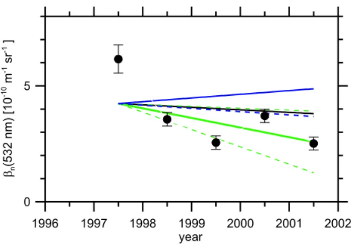
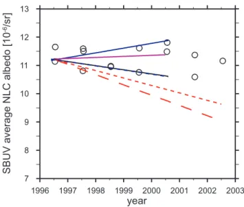
![Table 4. Observed ratios F and R for decadal NLC variations and β in units of [10 −10 m −1 sr −1 ].](https://thumb-eu.123doks.com/thumbv2/123doknet/14774582.593038/14.892.108.783.132.247/table-observed-ratios-f-decadal-nlc-variations-units.webp)
Documents relatifs
strip in good photometric conditions but having too few standard star measurements to perform the calibration may induce alone this offset; the equal number of detected objects as
From the top to the base, these formations are the Grès à Voltzia and the Couches Intermédiaires in the Upper Buntsandstein, the Poudingue de Sainte Odile, the Couches de Karlstal,
The first African ambers known to yield arthropods and other organismal inclusions, found recently from the early Cretaceous of Congo and the Miocene of Ethiopia, are brie
Pour résumer, nous avons reproduit le renfor ement à la traversée du y lone de surfa e, observé notamment dans le as de la POI17, dans le adre idéalisé d'un modèle à deux ou
Notre travail n’a pas traité directement de la synthèse de gestes plausibles. Notre objectif premier était de fournir un système capable de contrôler un robot
Il est co-auteur, avec Alain Beltran, d’une histoire de l’INRIA (His- toire d’un pionnier de l’informatique. 40 ans de recherche à l’INRIA, EDP Sciences, 2007)..
Phasico-tonic CBTs present a phasic firing, during release ramps, and develop a tonic discharge for the most released position of the CBCO strand. A: The first
Various cobalt mineralization styles on Earth can not be attributed to a single ore-forming model. At Bou Azzer, two types of ore bodies occur – “contact” and
